Constant Delay and Constant Feedback Moving Window Network Coding for Wireless Multicast: Design and Asymptotic Analysis

Fei Wu Yin Sun Yang Yang Kannan Srinivasan Ness B. Shroff ^†^†thanks: Fei Wu, Yin Sun, and Yang Yang are with the Department of ECE, The Ohio State University, Columbus, OH, 43210 (e-mail: wuff.gewuer@gmail.com, sunyin02@gmail.com, yang.1267@osu.edu).^†^†thanks: Kannan Srinivasan is with the Department of CSE, The Ohio State University, Columbus, OH, 43210 (e-mail: kannan@cse.ohio-state.edu).^†^†thanks: Ness B. Shroff is with the Departments of ECE and CSE, The Ohio State University, Columbus, OH, 43210 (e-mail: shroff.11@osu.edu).

Abstract

A major challenge of wireless multicast is to be able to support a large number of users while simultaneously maintaining low delay and low feedback overhead. In this paper, we develop a joint coding and feedback scheme named Moving Window Network Coding with Anonymous Feedback (MWNC-AF) that successfully addresses this challenge. In particular, we show that our scheme simultaneously achieves both a constant decoding delay and a constant feedback overhead, irrespective of the number of receivers $n$ , without sacrificing either throughput or reliability. We explicitly characterize the asymptotic decay rate of the tail of the delay distribution, and prove that transmitting a fixed amount of information bits into the MWNC-AF encoder buffer in each time-slot (called “constant data injection process”) achieves the fastest decay rate, thus showing how to obtain delay optimality in a large deviation sense. We then investigate the average decoding delay of MWNC-AF, and show that when the traffic load approaches the capacity, the average decoding delay under the constant injection process is at most one half of that under a Bernoulli injection process. In addition, we prove that the per-packet encoding and decoding complexity of MWNC-AF both scale as $O(\log n)$ , with the number of receivers $n$ . Our simulations further underscore the performance of our scheme through comparisons with other schemes and show that the delay, encoding and decoding complexity are low even for a large number of receivers, demonstrating the efficiency, scalability, and ease of implementability of MWNC-AF.

Index Terms:

Wireless multicast, low delay, low feedback, scaling law analysis.

I Introduction

Wireless multicast has numerous applications: wireless IPTV, distance education, web conference, group-oriented mobile commerce, firmware reprogramming of wireless devices, etc, [1, 2, 3]. However, in reality, there are only a few deployments. A major challenge that wireless multicast techniques have so far not been able to overcome is to achieve low delay without incurring a large amount of feedback. In the literature, there are two categories of multicast coding strategies. The first category focuses on batch-based coding schemes, e.g., random linear network coding (RLNC) [4], LT codes [5], and Raptor codes [6]. In these schemes, the transmitter sends out a linear combination generated from a batch of $B$ data packets in each time-slot. A new batch of packets cannot be processed until all the receivers have successfully decoded the previous packet batch. This approach has a low feedback overhead: one bit of acknowledgment (ACK) is sufficient to signal the decoding fate of an entire batch. However, with a fixed batch size, the achievable throughput decreases with the number of receivers $n$ . To maintain a fixed throughput, the batch size $B$ needs to grow on the order of $O(\log n)$ [7, 8]. As the batch size $B$ increases, the decoding delay also grows as $O(\log n)$ . Thus, such schemes achieve low feedback overhead at the cost of high decoding delay.

The second category of studies are centered on an incremental network coding design¹¹ 1 They are also referred as online or adaptive network coding in the literatures., e.g., [9, 10, 11, 12, 13, 14, 15, 16, 17, 18, 19, 20, 21, 22, 23, 24], where the data packets participate in the coding procedure progressively. Therefore, the receivers that have decoded old packets can have early access to the processing of new data packets, instead of waiting for all the other receivers to decode the old packets. The benefit of this approach is low decoding delay. Some studies have even shown a constant upper bound of decoding delay for any number of receivers, when the encoder is associated with a Bernoulli packet injection process [11, 18]. However, these schemes need to collect feedback information from all receivers, and the total feedback overhead increases with the number of receivers $n$ . Thus, these incremental-coding schemes achieve low delay, but at the cost of high feedback overhead.

Can we achieve the best of both worlds? This paper develops a joint coding and feedback scheme called Moving Window Network Coding with Anonymous Feedback (MWNC-AF) that achieves the delay performance of incremental-coding techniques without requiring the feedback overhead to scale with the number of receivers, as in the batch-based coding techniques. Hence, it indeed shows that the best of both worlds is achievable. We present a comprehensive analysis of the decoding delay, feedback overhead, encoding and decoding complexity of MWNC-AF. The contributions of this paper are summarized as follows:

•

We develop a joint coding and feedback scheme called MWNC-AF, and show that MWNC-AF achieves both a constant decoding delay and a constant feedback overhead²² 2 By constant delay and constant feedback overhead, we mean that the delay experienced by any receiver and the overall feedback overhead of all receivers are both independent of the number of receivers $n$ ., irrespective of the number of receivers $n$ , without sacrificing either throughput or reliability.
•

We investigate how to control the data injection process at the encoder buffer to reduce the decoding delay of MWNC-AF. To that end, we explicitly characterize the asymptotic decay rate of the tail of the decoding delay distribution for any i.i.d. data injection process. We show that injecting a constant amount of information bits into the encoder buffer in each time-slot (called “constant data injection process”) achieves the fastest decay rate, thus showing how to obtain delay optimality in a large deviation sense. (Theorem 1)
•

We derive an upper bound of the average decoding delay for MWNC-AF under the constant data injection process. As the traffic load approaches capacity, this upper bound is at most one half of the average decoding delay achieved by a Bernoulli data injection process. (Theorem 2)
•

For the constant data injection process, we prove that the average encoding complexity of MWNC-AF is of the form $\frac{1}{\eta}\log n+o(\log n)$ for sufficiently large $n$ , and the value of the pre-factor $\eta$ is attained as a function of the channel statistics and the injection rate. For any $n$ , we also characterize the asymptotic decay rate of the tail of the encoding complexity distribution. (Theorem 3)
•

For the constant data injection process, we prove that the average decoding complexity of MWNC-AF per data packet is also of the form $\frac{1}{\eta}\log n+o(\log n)$ for sufficiently large $n$ , and the pre-factor $\frac{1}{\eta}$ is the same as that of the average encoding complexity. (Theorem 4)

The rest of this paper is organized as follows. In Section II, we introduce some related work. In Section III, we describe the system model and present our MWNC-AF transmission design. In Section IV, we analyze the decoding delay, encoding complexity, and decoding complexity of the MWNC-AF transmission design. In Section V, we use simulations to verify our theoretical results. Finally, in Section VI, we conclude the paper.

II Related Work

Batch-based rateless codes can generate a potentially unlimited stream of coded packets from a fixed batch of data packets. The coded packets can be generated on the fly, as few or as many as needed [5]. Examples of Batch-based rateless codes includes random linear network coding (RLNC) [4], LT codes [5], and Raptor codes [6]. RLNC³³ 3 By RLNC, we refer to the specifications in [4, 25, 7]. is the simplest rateless codes, which can achieve near-zero communication overhead. However, the decoding complexity of RLNC is high [26] for large block size $B$ . LT codes and Raptor codes were proposed to reduce the decoding complexity. In particular, Raptor codes can achieve constant per-packet encoding and decoding complexity. One benefit of batch-based rateless codes is low feedback overhead [27]. A feedback scheme was proposed in [28] for RLNC, which has a constant overhead independent of the number of receivers. However, these schemes have poor delay performance when the number of receivers $n$ is large. Recent analyses have shown that, to maintain a fixed throughput, the batch size in these schemes needs to grow with respect to the number of receivers $n$ , which results in a long decoding delay [7, 8]. Scheduling techniques have been developed to optimize the tradeoff between the batch size and throughput under limited feedback for finite $n$ [29, 30]. However, it is difficult to maintain a low decoding delay for large $n$ , unless resorting to novel coding designs.

In recent years, a class of incremental network coding schemes, e.g., [9, 10, 11, 12, 13, 14, 15, 16, 17, 18, 19, 20, 21, 22, 23, 24] are developed to resolve the long decoding delay of rateless codes. In these designs, the data packets participate in the coding procedure progressively. Among this class, an instantly decodable network coding scheme was proposed in [13, 14], where the number of receivers that can be effectively supported is maximized under a zero decoding delay constraint. In order to accommodate more receivers, the zero decoding delay constraint was relaxed in [15]. Nonetheless, these schemes cannot support a large number of receivers.

A number of ARQ-based network coding schemes are proposed since the seminal work [10, 11], which can potentially reduce the decoding delay and support a large number of receivers. In [10, 11], the desired packet of each receiver is acknowledged to the transmitter, such that the transmitted packet is a linear combination of the desired packets of all receivers. Without appropriate injection control, this scheme results in unfair decoding delay among the receivers with different packet erasure probabilities. A threshold-based network coding scheme was proposed in [12] to resolve this fairness issue, at the cost of some throughput loss. A dynamic ARQ-based network coding scheme was proposed in [18], which can achieve noticeable improvement in the throughput-delay tradeoff performance. Interestingly, when associated with a Bernoulli packet injection process, the average decoding delay of ARQ-based network coding is upper bounded by a constant⁴⁴ 4 When the number of receivers $n$ is small, the average decoding delay in [11, 18] can be substantially smaller than the upper bound. However, when there are a large number of receivers, the average decoding delay in [11, 18] is very close to the upper bound, as shown in [18]. independent of the number of receivers $n$ [11, 18]. However, these schemes require explicit feedback from each receiver, and thus their feedback overhead scales up with the number of receivers $n$ . A generalization of ARQ-based network coding was the moving window network coding (MWNC), which was first proposed in [21] to make network coding compatible with the existing TCP protocol. The MWNC scheme was also employed in multihop wireless networks to improve the throughput of opportunistic routing [22] and support multiple multicast sessions [23]. However, in these designs, the movement of the encoding window requires the ACK from all receivers, and thus the feedback overhead scales up with the network size.

Recently, the first author proposed an anonymous feedback scheme for MWNC [19], which can achieve a constant feedback overhead for any number of receivers $n$ . However, this feedback scheme assumed that all receivers are within a short range of each other and can communicate with one another, which may introduce the well-known hidden terminal problem in practical systems. In addition, the window size of the MWNC scheme was fixed in [19], which leads to a throughput degradation as the number of receivers $n$ grows up. Another low-overhead feedback scheme was proposed in [20] for ARQ-based network coding, where only the leading and tail receivers feed back messages to the transmitter. However, it was not discussed in [20] whether their scheme can achieve constant decoding delay for any number of receivers. To the extent of our knowledge, no previous scheme exists that can simultaneously guarantee constant decoding delay and constant feedback overhead as the number of receivers $n$ grows, without sacrificing the throughput and reliability of wireless multicast.

III System Model

III-A Channel Model

We consider a broadcast packet erasure channel with one transmitter and $n$ receivers, where the transmitter needs to send a stream of common information to all the receivers.

We assume a time-slotted system. In each time-slot, the transmitter generates one coded packet and broadcasts it to all the receivers. The channel from the transmitter to the receiver $i$ in time-slot $t$ is denoted as $c_{i}[t]$ , where

\displaystyle\!\!\!\!c_{i}[t]=\left\{\begin{array}[]{ll}1&\text{if a coded packet is successfully}\\ &\text{received by receiver $i$ at time-slot $t$;}\\ 0&\text{otherwise.}\end{array}\right.\vskip 8.5359pt

We assume that $c_{i}[t]$ is i.i.d. across time-slots, and define $\gamma_{i}\triangleq\mathbb{P}\left(c_{i}[t]=1\right)$ . Then, the capacity of this broadcast channel is $\inf_{1\leq i\leq n}\gamma_{i}$ packets per time-slot.

It is assumed that on the feedback channel, the transmitter and each receiver can overhear each other, but the receivers may not overhear each other. Since all receivers are within the one-hop transmission range of the transmitter and in practice the feedback signals are usually sent at a much lower data rate than the normal data packet, similar to [9, 10, 11, 12, 13, 14, 15, 16, 17, 18, 19, 20, 21, 22, 23, 28], we assume that the feedback signals can be reliably detected.

III-B Multicast Transmission Design

We propose a multicast transmission scheme called moving window network coding with anonymous feedback (MWNC-AF). This scheme achieves a constant decoding delay and a constant feedback overhead for any number of receivers $n$ .

III-B1 Encoder

Assume that the transmitter is infinitely backlogged, and that $\tilde{a}[t]$ bits are injected to the encoder buffer from the backlog at the beginning of time-slot $t$ . The bits received by the encoder are assembled into packets of $L$ bits. Let us define $a[t]={\tilde{a}[t]}/{L}$ , which is a rational number. We assume that $a[t]$ is i.i.d. across time-slots with mean $\lambda\triangleq\mathbb{E}\left[a[t]\right]$ . Then, the number of packets that the encoder has received up to the beginning of time-slot $t$ is $A[t]$ , i.e.,

\displaystyle A[t]=\sum_{\tau=1}^{t}a[\tau].

(4)

We note that only fully assembled packets can participate the encoding operation. The number of fully assembled packets up to the beginning of time-slot $t$ is $\left\lfloor A[t]\right\rfloor$ , where $\lfloor y\rfloor$ is the maximum integer no greater than $y$ .

Let $Z[t]\in\mathbb{N}$ denote the number of packets that have been removed from the encoder buffer by the end of slot $t$ . The evolution of $Z[t]$ will be explained in Section III-B3, along with the anonymous feedback scheme. The coded packet $x[t]$ in time-slot $t$ is generated by

\displaystyle x[t]=\sum_{m=Z[t-1]+1}^{\left\lfloor A[t]\right\rfloor}\alpha_{t,m}\times p_{m},

(5)

where $p_{m}$ denotes the $m^{\text{th}}$ assembled packet of the encoder, “ $\times$ ” is the product operator on a Galois field $GF(2^{q})$ , and $\alpha_{t,m}$ is randomly drawn according to a uniform distribution on $\{GF(2^{q})\}\backslash\{0\}$ .⁵⁵ 5 The bit-size $L$ of each packet is a multiple of $q$ . The values of $\left\lfloor A[t]\right\rfloor$ and $Z[t-1]$ are embedded in the packet header of $x[t]$ . In addition, $\{\alpha_{t,m}\}$ are known at each receiver by feeding the same seed to the random number generators of the transmitter and all the receivers.

Let $W[t]$ denote the number of packets that participate in the encoding operation of $x[t]$ in time-slot $t$ , which is called encoder queue length or encoding window size in this paper. According to Equation (5), $W[t]$ is determined by

\displaystyle W[t]

\displaystyle=\left\lfloor A[t]\right\rfloor-Z[t-1].

(6)

III-B2 Decoder

Fig. 1: An example for the decoding procedure of MWNC-AF.

To facilitate a clear understanding of the decoding procedure, we restate the definition of a user seeing a packet that was originally described in [10].

Definition 1.

(Seeing a packet) We say that a receiver has “seen” a packet $p_{m}$ , if it has enough information to express $p_{m}$ as a linear combination of some packets $p_{m+1},p_{m+2},\cdots$ with greater indices.

We first use the example illustrated in Fig. 1 to explain the decoding procedure. In this example, the coded packets $x[1]$ , $x[2]$ , $x[3]$ , and $x[4]$ are successfully delivered to a certain receiver in time slots 1-4, respectively. In time-slot 1, packet $p_{1}$ is “seen” at the receiver, because it can be expressed as

p_{1}=x[1]-p_{2}.

Similarly, in time slots 2-4, packets $p_{2}$ , $p_{3}$ , and $p_{4}$ are “seen” one by one, because they can be expressed as

	$\displaystyle p_{2}=x[2]-x[1]-p_{4}-p_{3},$
	$\displaystyle p_{3}=x[3]-x[2]+x[1]-2p_{4},$
	$\displaystyle p_{4}=-x[4]+x[3]-x[2]+x[1].$

Now, packet $p_{4}$ is immediately decoded, because $x[1]$ , $x[2]$ , $x[3]$ , and $x[4]$ are available at the receiver. Once $p_{4}$ is decoded, it can be substituted backwards to decode $p_{3}$ , $p_{2}$ , and $p_{1}$ one by one.

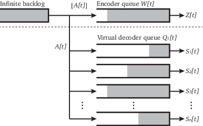
Let $S_{i}[t]\in\mathbb{N}$ be the number of packets that receiver $i$ has “seen” by the end of time-slot $t$ . Define a virtual decoder queue

\displaystyle Q_{i}[t]=A[t]-S_{i}[t]

(7)

for each receiver $i$ . Then, $\left\lfloor Q_{i}[t]\right\rfloor$ is the number of “unseen” packets at receiver $i$ at the end of time-slot $t$ .

The decoding procedure of receiver $i$ is described as follows:

At the beginning of time-slot $t$ , receiver $i$ has seen the packets $p_{1},\cdots,p_{S_{i}[t-1]}$ . Suppose $c_{i}[t]=1$ , which implies that packet $x[t]$ is successfully delivered to receiver $i$ in time-slot $t$ . If $A[t]-S_{i}[t-1]\geq 1$ , the packets participated in generating $x[t]$ contains at least one “unseen” packet $p_{S_{i}[t-1]+1}$ . Receiver $i$ eliminates the “seen” packets $p_{1},\cdots,p_{S_{i}[t-1]}$ from the expression of $x[t]$ in Equation (5) of $x[t]$ , to obtain an expression of $p_{S_{i}[t-1]+1}$ . If the field size $2^{q}$ is sufficiently large, then with high probability, packet $p_{S_{i}[t-1]+1}$ can be expressed as a linear combination of the packets $p_{S_{i}[t-1]+2},p_{S_{i}[t-1]+3},\cdots$ with greater indices. In other words, packet $p_{S_{i}[t-1]+1}$ is “seen” in time-slot $t$ . Therefore, the value of $S_{i}[t]$ can be updated by

\displaystyle S_{i}[t]=S_{i}[t-1]+c_{i}[t]1_{\left\{A[t]-S_{i}[t-1]\geq 1\right\}},

(8)

where ${1}_{A}$ is the indicator function of event $A$ .

\displaystyle\left\lfloor A[t]\right\rfloor=S_{i}[t]\text{~or~equivalently~}\left\lfloor Q_{i}[t]\right\rfloor=0,

(9)

i.e., receiver $i$ has “seen” all the packets that participated in the encoding operation of $x[t]$ , then receiver $i$ can decode packet $p_{S_{i}[t]}$ . Once $p_{S_{i}[t]}$ is decoded, it can be substituted backwards to sequentially decode $p_{S_{i}[t]-1}$ , $p_{S_{i}[t]-2}$ , $\cdots$ , for all “seen” packets.

III-B3 Anonymous Feedback

According to the decoding procedure, if a packet $p_{m}$ is “unseen” at some receiver $i$ , it cannot be removed from the encoder buffer. Because, otherwise, receiver $i$ will never be able to “see” packet $p_{m}$ or decode it. In order to ensure reliable multicast, the departure process $Z[t]$ of the encoder buffer should satisfy

\displaystyle Z[t]\leq\min_{1\leq i\leq n}S_{i}[t].

(10)

Algorithm 1 Beacon-based Anonymous Feedback

Feedback procedure of receiver

i

{Z}_{i}[0]:=0

;

S_{i}[0]:=0

;

for time slot $t=1:\infty$ do - - - - - - - Data sub-slot - - - - - - - - - -

Receive coded packet

x[t]

;

Update

S_{i}[t]

according to Equation (8);

- - - - - - - Beacon sub-slot - - - - - - - -

if $S_{i}[t]=Z_{i}[t-1]$ then Send out a beacon signal;

{Z}_{i}[t]:={Z}_{i}[t-1]

;

else Detect beacon signal;

if no beacon signal is detected then

{Z}_{i}[t]:={Z}_{i}[t-1]+1

;

else

{Z}_{i}[t]:={Z}_{i}[t-1]

;

endif endif

end Reaction procedure of the transmitter:

Z[0]:=0

;

for time slot $t=1:\infty$ do - - - - - - - Data sub-slot - - - - - - - - - -

Send coded packet

x[t]

;

- - - - - - - Beacon sub-slot - - - - - - - - -

Detect beacon signal;

if beacon signal is detected then Send out a beacon signal;

Z[t]:=Z[t-1]

;

else

Z[t]:=Z[t-1]+1

;

Remove the oldest packet from the encoder;

endif end

We now provide a beacon-based anonymous feedback scheme, provided in Algorithm 1. In this algorithm, receiver $i$ maintains a local parameter $Z_{i}[t]$ , which is synchronized with $Z[t]$ at the transmitter through beacon signaling. Each time-slot is divided into a long data sub-slot and a short beacon sub-slot. In the data sub-slot, the transmitter broadcasts a data packet to all the receivers. Then, $S_{i}[t]$ is updated according to Equation (8). In the beacon sub-slot, if receiver $i$ finds that $S_{i}[t]=Z_{i}[t-1]$ , it sends out a beacon signal in the common feedback channel, requesting the transmitter not to remove the oldest packet in the encoder buffer. If the transmitter has detected the beacon signal (from one or more receivers), the transmitter will broadcast a beacon signal instantly within the same beacon sub-slot, and no packet will be removed from the encoder buffer, i.e.,

\displaystyle Z[t]=Z[t-1].

(11)

In the beacon sub-slot, the transmitter serves as a relay for the beacon signal. This second beacon transmission guarantees that receivers that are hidden from each other can still detect each other¡¯s beacon signal. If the transmitter has detected no beacon signal, it will remove the oldest packet in the encoder buffer, i.e.,

\displaystyle Z[t]=Z[t-1]+1.

(12)

By detecting the existence of beacon signal in the beacon-sub-slot, each receiver synchronizes $Z_{i}[t]$ with $Z[t]$ . A key benefit of this anonymous feedback scheme is that its overhead (i.e., one short beacon sub-slot) is constant for any number of receivers n.

Refer to caption — Fig. 2: The queueing model for MWNC-AF.

Lemma 1.

The beacon-based anonymous feedback Algorithm 1 satisfies

\displaystyle Z[t]=\min_{1\leq i\leq n}S_{i}[t],

(13)

for all time-slots $t$ .

Proof.

See Appendix F. ∎

Therefore, this anonymous feedback scheme not only ensures reliable multicast, but also keeps the encoder buffer as small as possible.

Remark 1.

In practice, the length of beacon sub-slot should take into account the round-trip time of the beacon signal, and the delay due to the signal detection or the hardware reaction time. Although the beacon sub-slots are reserved in this paper, anonymous feedback can also be implemented on a dedicated feedback channel of orthogonal frequency.

It is important to note that the overhead of the anonymous feedback can be significantly reduced by performing feedback only once for every $B_{AF}$ time slots. The details of infrequent anonymous feedback for MWNC will be discussed in Section IV-D.

Equations (8) and (13) tell us that

\displaystyle Z[t-1]\leq\min_{1\leq i\leq n}S_{i}[t]\leq Z[t-1]+1.

(14)

Moreover, we have

\displaystyle\left\lfloor A[t]\right\rfloor\leq A[t]\leq\left\lfloor A[t]\right\rfloor+1.

(15)

Combining Equations (6), (7), (14) and (15), it is easy to derive

\displaystyle\max_{1\leq i\leq n}Q_{i}[t]-1\leq W[t]\leq\max_{1\leq i\leq n}Q_{i}[t]+1.

(16)

The relationship between the encoding window size $W[t]$ and the decoder queue $Q_{i}[t]$ is depicted in Fig. 2, as will be clarified subsequently. One can observe that the difference between the encoder queue length $W[t]$ and the maximum decoder queue length $\max_{1\leq i\leq n}Q_{i}[t]$ is quite small.

In order to keep the queueing system stable, we assume that the average injection rate $\mathbb{E}\{a[t]\}=\lambda$ is smaller than the capacity, i.e., $\lambda<\inf_{1\leq i\leq n}\gamma_{i}$ for any number of receivers $n$ . We define $\gamma\triangleq\inf\{\gamma_{i},i=1,2,\cdots\}>0$ as a lower bound of the multicast capacity for all $n$ , and $\rho\triangleq\frac{\lambda}{\gamma}$ as the traffic intensity of the system satisfying $\rho<1$ .

IV Performance Analysis of MWNC-AF

In this section, we rigorously analyze the decoding delay, encoding complexity, and decoding complexity of MWNC-AF for a given throughput $\mathbb{E}[a[t]]=\lambda~\text{packet}/\text{slot}$ .

IV-A Decoding Delay

Let the time-slots $t_{i}^{j}$ $(j=1,2,\cdots)$ be the decoding moments of receiver $i$ satisfying Equation (9). Suppose that packet $p_{m}$ is assembled at the encoder buffer in time-slot $t$ , which is between two successive decoding moments $t_{i}^{j}<t\leq t_{i}^{j+1}$ . Then, packet $p_{m}$ will be decoded in time-slot $t_{i}^{j+1}$ . The decoding delay of packet $p_{m}$ at the receiver $i$ is

\displaystyle D_{i,m}=t_{i}^{j+1}-t.

(17)

Then, assuming the system is stationary and ergodic, the delay violation probability that the decoding delay of a packet exceeds a threshold $k$ is expressed as

\displaystyle\mathbb{P}(D_{i}>k)=\lim_{M\to\infty}\frac{1}{M}\sum_{m=1}^{M}{1}_{\{D_{i,m}>k\}}.

(18)

The average decoding delay of receiver $i$ is given by

\displaystyle\overline{D}_{i}=\lim_{M\to\infty}\frac{1}{M}\sum_{m=1}^{M}D_{i,m}.

(19)

Theorem 1.

In a network with $n$ receivers, if the data injections $a[t]$ are i.i.d. across time-slots with an average rate $\mathbb{E}[a[t]]=\lambda$ and $\lambda<\gamma$ , then for any receiver $i$ , the asymptotic decay rate of the delay violation probability of MWNC-AF is

-\lim_{k\to\infty}\frac{1}{k}\log\mathbb{P}(D_{i}>k)=\Phi_{i},

where $\log(\cdot)$ denotes natural logarithm and

\displaystyle\Phi_{i}=\sup_{\theta\in\mathbb{R}}\left\{-\log\mathbb{E}\left(e^{-\theta a[t]}\right)-\log\left(\gamma_{i}e^{\theta}+1-\gamma_{i}\right)\right\}.

(20)

In addition,

\displaystyle\Phi_{i}\leq\lambda_{i}\log\frac{\lambda}{\gamma_{i}}+(1-\lambda)\log\frac{1-\lambda}{1-\gamma_{i}},

where the equality holds if $a[t]=\lambda$ for all $t$ .

Proof.

See Appendix B. ∎

Theorem 1 has characterized the asymptotic decay rate of the delay violation probability $\mathbb{P}(D_{i}>k)$ of receiver $i$ as $k$ increases. It tells us that a constant packet injection process, i.e.,

\displaystyle a[t]=\lambda,~\forall~t,

(21)

achieves the fastest decay rate among all i.i.d. packet injection processes. We note that the decoding delay of receiver $i$ is independent of the channel condition $\gamma_{j}$ ( $j\neq i$ ) of other receivers. The reason for this is the following: By Equation (9), the decoding moment of receiver $i$ is determined by $\left\lfloor Q_{i}[t]\right\rfloor=0$ . Further, according to Equations (4), (7), and (8), the evolutions of $Q_{i}[t]$ depend on the common data injection process $A[t]$ and channel conditions $c_{i}[t]$ of receiver $i$ , both of which is independent of $\gamma_{j}$ for $j\neq i$ . In [24], the authors derived the same expression of the delay’s decay rate for the constant injection process, which is a special case of our result.

Theorem 2.

In a network with $n$ receivers, if the amount of packet injected in each time-slot is $a[t]=\lambda$ for all $t$ and $\lambda<\gamma$ , then for any receiver $i$ , the average decoding delay of MWNC-AF is upper bounded by

\displaystyle\overline{D}^{\text{Con}}_{i}\leq\frac{\gamma_{i}(1-\gamma_{i})}{2(\gamma_{i}-\lambda)^{2}}+\frac{1}{\gamma_{i}-\lambda}+\frac{5}{2\lambda}.

(22)

In addition, as $\rho$ increases to $1$ , $\overline{D}^{\text{Con}}_{i}$ is asymptotically upper bounded by

\displaystyle\lim_{\rho\to 1^{-}}\frac{\overline{D}_{i}^{\text{Con}}}{1/(1-\rho)^{2}}\leq\frac{1-\gamma}{2\gamma}.

(23)

Proof.

See Appendix C. ∎

The analysis of [11] implies that, under a Bernoulli packet injection process, i.e.,

\displaystyle\mathbb{P}(a[t]=1)=\lambda,~~\mathbb{P}(a[t]=0)=1-\lambda,

(24)

the average decoding delay $\overline{D}_{i}^{\text{Ber}}$ of the receiver $i$ with $\gamma_{i}=\gamma$ satisfies

\displaystyle\lim_{\rho\to 1^{-}}\frac{\overline{D}_{i}^{\text{Ber}}}{1/(1-\rho)^{2}}=\frac{1-\gamma}{\gamma}.

(25)

This and (23) tell us that for the bottleneck receiver(s), the average decoding delay under a constant injection process is at most one half of that of the Bernoulli packet injection process as $\rho$ approaches $1$ .

It is known that the average decoding delay of batch-based rateless codes scales up at a speed no smaller than $O(\log n)$ , as the number of receivers $n$ increases [7, 8]. Theorems 1 and 2 tell us that the decoding delay of MWNC-AF remains constant for any number of receiver $n$ . The average decoding delay performance of two ARQ-based coding schemes in [11, 18] is also bounded by some constant independent of $n$ . As we have mentioned, the overhead of our anonymous feedback mechanism remains constant for any number of receiver $n$ . But the feedback overhead of the schemes in [11, 18] scales up as $n$ increases.

IV-B Encoding Complexity

We count one operation as one time of addition and multiplication on the Galois field. According to (5) and (6), the encoding complexity of packet $x[t]$ is ${W}[t]$ , i.e., the number of fully assembled packets in the encoder buffer. For any given number of receivers $n$ , the average encoding complexity of MWNC-AF to encode one coded packet is

\displaystyle\overline{W}_{n}=\lim_{M\to\infty}\frac{1}{M}\sum_{t=1}^{M}{W}[t],

(26)

In addition, the probability that the encoding complexity of MWNC-AF exceeds a threshold $k$ is depicted by

\displaystyle\mathbb{P}(W_{n}>k)=\lim_{M\to\infty}\frac{1}{M}\sum_{t=1}^{M}{1}_{\{W[t]>k\}}.

(27)

Theorem 3.

In a network with $n$ receivers, if the amount of packet injected in each time-slot is $a[t]=\lambda$ for all $t$ and $\lambda<\gamma$ , then the average encoding complexity of MWNC-AF satisfies

\lim_{n\to\infty}\frac{\overline{W}_{n}}{\log n}\leq\frac{1}{\eta},

(28)

where

\displaystyle\eta=\log\frac{\gamma e^{\theta}}{1-(1-\gamma)e^{\theta}},

(29)

and $\theta$ is the unique solution of the equation

\displaystyle e^{-\frac{\theta}{\lambda}}\cdot\frac{\gamma e^{\theta}}{1-(1-\gamma)e^{\theta}}=1,\quad 0<\theta<-\log(1-\gamma).

(30)

The asymptotic decay rate of the probability that the encoding complexity exceeds a threshold is lower bounded by

\displaystyle-\lim_{k\to\infty}\frac{1}{k}\log\mathbb{P}\left(W_{n}>k\right)\geq\eta.

(31)

The inequalities in Equations (28) and (31) become equalities when $\gamma_{1}=\dots=\gamma_{n}=\gamma$ .

Proof.

See Appendix D. ∎

Theorem 3 tells us that the average encoding complexity of MWNC-AF increases as $O(\log n)$ when $n$ increases, and the asymptotic decay rate of the encoding complexity of MWNC-AF does not depend on $n$ .

In [31], it was shown that, for any coding scheme of wireless multicast, the average encoder queue length must scale up at a speed no slower than $O(\log n)$ as $n$ increases. This, together with Theorem 3, tells us that MWNC-AF has achieved the optimal scaling law of the average encoder queue length. Interestingly, in MWNC-AF, a large encoder queue length does not necessarily transform into a long decoding delay, because the encoder buffer contains both the packets that have and have not been decoded by each receiver.

According to [31], the encoder queue length of RLNC also grows at a speed of $O(\log n)$ .

It is worthwhile to mention that from Equation (31), the probability that the encoder queue size $W[t]$ exceeds a threshold $k$ decays exponentially when $k$ is sufficiently large. Therefore, the encoder queue size $W[t]$ is unlikely to be much greater than its average value.

IV-C Decoding Complexity

For any given number of receivers $n$ , the average decoding complexity $\Omega_{n}$ of MWNC-AF is measured by the average number of operations for decoding one data packet at each receiver.

Theorem 4.

In a network with $n$ receivers, if the amount of packets injected in each time-slot is $a[t]=\lambda$ for all $t$ and $\lambda<\gamma$ , then the average decoding complexity of MWNC-AF, denoted as $\overline{\Omega}_{n}$ , satisfies

\displaystyle\lim_{n\to\infty}\frac{\overline{\Omega}_{n}}{\log n}\leq\frac{1}{\eta},

(32)

where $\eta$ is defined in Equation (29).

The inequality in Equation (32) becomes equalities when $\gamma_{1}=\dots=\gamma_{n}=\gamma$ .

Proof.

See Appendix E. ∎

Theorem 4 has characterized the average decoding complexity of MWNC-AF. Interestingly, we can observe from Equations (28) and (32) that both the average encoding and the average decoding complexity are of the form $\frac{1}{\eta}\log n+o(\log n)$ .

For RLNC, in order to maintain a constant throughput $\lambda>0$ as the number of receivers $n$ increases, the average decoding complexity of RLNC needs to increase at a rate no slower than $O((\log n)^{2})$ .⁶⁶ 6 The reason for this is as follows: Consider a RLNC code with a block size of $B$ data packets. Its average decoding complexity for each packet is of the order $O(B^{2})$ , as shown in [32]. On the other hand, it was shown in [7] that in order to maintain a constant throughput $\lambda>0$ as $n$ increases, the block size $B$ must scale up at a speed of $O(\log n)$ . This and Theorem 4 tell us that the average decoding complexity of MWNC-AF scales much slower than that of RLNC.

IV-D MWNC with Infrequent Anonymous Feedback

So far, the anonymous feedback is performed on a per-packet basis. Although the feedback overhead has been a constant independent of the number of receivers, implementing feedback for every time slot may still consume nonnegligible bandwidth resources. In this subsection, we show that by infrequent anonymous feedback, the feedback overhead can be conceptually reduced to $1/B_{AF}$ of that of the original MWNC-AF, and meanwhile neither the delay nor the reliability at the receivers is jeopardized. The costs for the further reduction of feedback overhead are the increased encoding and decoding complexity. The infrequent anonymous feedback provides a tradeoff between computation complexity and feedback overhead for MWNC-AF.

In this policy, anonymous feedback is practiced once for a frame of $B_{AF}$ packet transmissions, as shown in Figure 3. If the transmitter cannot detect the beacon signal, it will remove $B_{AF}$ packets from the encoder buffer at the end of the frame. Otherwise, no packet will be removed. We can ensure that the removed packets are already “seen” at each receiver, i.e., the multicast transmissions are reliable. We note that this policy does not increase the decoding delay, because the decoding delay is determined by the virtual decoder queue $Q_{i}[t]$ of each receiver, and does not depend on the encoder queue $W[t]$ .

Due to the infrequent removal of packets in the encoder, the average encoding as well as decoding complexity of MWNC-AF with $B_{AF}>1$ would be greater than the case when $B_{AF}=1$ . However, it is straightforward to see that with infrequent anonymous feedback, the average encoding complexity is at most $B_{AF}$ more than the average encoding complexity of the original MWNC-AF, i.e., $\overline{W}_{n}+B_{AF}$ .

V Numerical Results

This section presents some simulation results that provide insights and trends as well as validate the theoretical results. We investigate three important aspects of performance: decoding delay, encoding complexity, and decoding complexity. We consider two network scenarios, one with homogeneous channel conditions where $\gamma_{1}=\dots=\gamma_{n}=0.6$ , and the other with heterogenous channel conditions where $\gamma_{1}=\dots=\gamma_{n/2}=0.6$ and $\gamma_{n/2+1}=\dots=\gamma_{n}=0.8$ . The simulation results are derived by running over at least $10^{7}$ time-slots.

V-A Decoding delay

Since the delay performance for a receiver of MWNC-AF is uniquely determined by the injection process and the channel conditions of the receiver, we focus on a receiver with $\gamma_{i}=0.6$ . Figure 4 illustrates the delay violation probability $\mathbb{P}(D_{i}>k)$ of MWNC-AF versus $k$ . One can observe that the delay violation probability $\mathbb{P}(D_{i}>k)$ of MWNC-AF decays exponentially for sufficiently large $k$ and matches the predicted asymptotic decay rate from Equation (20). For $\lambda=0.5$ , as expected from our theoretical results, we find that a constant packet injection process achieves a much faster decay rate than the Bernoulli packet injection process. In addition, comparing the simulation results for $\lambda=0.5$ and $\lambda=0.54$ , the delay violation probability $\mathbb{P}(D_{i}>k)$ for a fixed $k$ increases with respect to $\lambda$ . Therefore, there is a tradeoff between system throughput and delay violation probability. One can utilize Equation (20) to search for the parameters $\lambda$ and $\gamma$ for achieving an appropriate delay-throughput tradeoff depending on design requirements.

Figure 5 plots the average decoding delay $\overline{D}_{i}$ of different network coding schemes versus the traffic intensity $\rho$ in the homogeneous network setting, where $n=100$ and $\gamma=0.6$ . One can observe the following results: First, the average decoding delay of RLNC [4] with batched packet arrivals is much larger than that of MWNC-AF. We note that the average decoding delay of LT codes [5], Raptor codes [6] are larger than that of RLNC, because of an extra reception overhead. Second, the average decoding delay of MWNC-AF with constant packet injections is much smaller than that of MWNC-AF with Bernoulli packet injections. When $\rho$ tends to 1, the constant packet injection process can reduce the average decoding delay of MWNC-AF by one half, over the Bernoulli packet injection process. Third, the average decoding delay of ARQ-based network coding (ANC) with dynamic injection control [18] is almost the same as that of MWNC-AF with constant packet injections. However, it is important to note that the scheme of [18] requires explicit feedback from each receiver, and thus its total feedback overhead grows as $O(n)$ . In comparison, the feedback overhead of MWNC-AF with constant packet injections remains the same, regardless of $n$ . Finally, the delay upper bound in Equation (22) for MWNC-AF with constant packet injections is accurate for high load.

V-B Encoding complexity

Figure 6 plots the probability $\mathbb{P}(W_{n}>k)$ of MWNC-AF versus $k$ for $\gamma=0.6$ . One can observe that $\mathbb{P}(W_{n}>k)$ decays exponentially for sufficiently large $k$ and matches the predicted asymptotic decay rate $\eta$ from Equation (29). Since $\eta$ is a decreasing function of $\rho$ and is irrelevant of $n$ , the traffic intensity $\rho$ has a larger impact on the probability $\mathbb{P}(W_{n}>k)$ than the number of receivers $n$ , when $k$ is sufficiently large. It can be also found that the decay rate of $\mathbb{P}(W_{n}>k)$ with the heterogeneous channel conditions is very close to that with the homogenous channel conditions.

In Fig. 7, we compare the average encoding complexity $\overline{W}_{n}$ of different network coding schemes versus the number of receivers $n$ , where $\rho=0.9$ and $\gamma=0.6$ . In the homogeneous network scenario, we find that the increasing rate of the average encoding complexity of MWNC-AF matches well with the predicted asymptotic rate even for relatively small $n$ . The expression $\frac{1}{\eta}\log n$ provides a close approximation of the average encoding complexity of MWNC-AF. One can also observe that the average encoding complexity of RLNC is of the order $O(\log n)$ , but its pre-factor is larger than that of MWNC-AF, i.e., $1/\eta$ . Therefore, the average encoding complexity of RLNC grows faster than that of MWNC-AF as $n$ increases. When $n=1024$ receivers, the average encoding complexity of MWNC-AF is less than 25. In the heterogenous network scenario, the average encoding complexity is less than but close to that in the homogenous network setting.

In Figure 8, we show the impact of infrequent anonymous feedback on the encoding complexity of MWNC-AF. It can be seen that the average encoding complexity increases almost linearly with respect to $B_{AF}$ . Even for 100 receivers with a load as high as 0.9, feedback can be performed only once in every 40 slots, at the same time less than 45 operations are needed on average to encode a packet.

V-C Decoding complexity

In Fig. 9, we compare the average decoding complexity $\overline{\Omega}_{n}$ of different network coding schemes with the number of receivers $n$ for $\rho=0.9$ and $\gamma=0.6$ . In the homogeneous network scenario, one can observe that the average decoding complexity of RLNC is much larger than that of MWNC-AF. Our simulation results suggest that the average decoding complexity of MWNC-AF grows as $O(\log n)$ . In particular, as $n$ grows from 2 to 1024, the average decoding complexity of MWNC-AF is only increased by 8 times. However, the pre-factor of the average decoding complexity of MWNC-AF has not converged to $1/\eta$ as $n$ grows to 1024. We believe that this convergence would occur at very large values of $n$ , which is beyond our current simulation capability. In the heterogenous network scenario, the average decoding complexity is less than that in the homogenous network setting.

Note that we have chosen a relative large value of $\rho$ (i.e., $\rho=0.9$ ) in Figs. 7 and 9. The average encoding and decoding complexity of MWNC-AF will be even smaller as $\rho$ decreases.

Lastly, in Figure 10, we show the impact of infrequent anonymous feedback on the decoding complexity of MWNC-AF. For a given $B_{AF}$ and $n$ , the average decoding complexity is larger than the average encoding complexity shown in Figure 8, and the difference is more evident for high load. Even for 100 receivers with a load as high as 0.9, feedback can be performed only once in every 40 slots, at the same time less than 80 operations are needed on average to decode a packet.

VI Conclusions

In this paper, we have developed a joint coding and feedback scheme called Moving Window Network Coding with Anonymous Feedback (MWNC-AF). We have rigorously characterized the decoding delay, encoding complexity, and decoding complexity of MWNC-AF. Our analysis has shown that MWNC-AF achieves constant decoding delay and constant feedback overhead for any number of receivers $n$ , without sacrificing the throughput and reliability of wireless multicast. In addition, we have proven that injecting a fixed amount of information bits into the MWNC-AF encoder buffer in each time-slot can achieve a much shorter decoding delay than the Bernoulli data injection process. We have also demonstrated that the encoding and decoding complexity of MWNC-AF grow as $O(\log n)$ as $n$ increases. Our simulations show that, for $n=1024$ receivers, the encoding and decoding complexity of MWNC-AF are still quite small. Therefore, MWNC-AF is suitable for wireless multicast with a large number of receivers.

Appendix A preliminaries

We first provide some preliminary results, which are helpful for our proofs.

According to Equations (4) and (7), we can derive

\displaystyle Q_{i}[t-1]+a[t]=A[t]-S_{i}[t-1].

(33)

Using this and (8), one can derive the evolutions of the decoder queue $Q_{i}[t]$ , given by

\displaystyle Q_{i}[t]=Q_{i}[t-1]+a[t]-c_{i}[t]1_{\left\{Q_{i}[t-1]+a[t]\geq 1\right\}}.

(34)

Accordingly, $\{Q_{i}[t]\}_{t}$ is a random walk on $[0,\infty)$ , which has a steady state distribution if $\lambda<\gamma_{i}$ .

Statement 1.

If the injection process is constant, i.e., $a[t]=\lambda$ for all $t$ , then the decoder queues $\left\{Q_{i}[t]\right\}_{1\leq i\leq n}$ are independent.

When $a[t]=\lambda$ for all $t$ , the injection and departure processes $\{a[t],c_{i}[t]\}_{t}$ are independent for different receivers. Then, Statement 1 follows from the queue evolution in Equation (34). For general packet injection processes, the decoder queues $\left\{Q_{i}[t]\right\}_{1\leq i\leq n}$ are correlated.

Next, we show that the decoding procedure for any receiver $i$ can be captured by a Markov renewal process. Since the system is symmetric, we only need to consider the decoding procedure at receiver 1. Let us define $T_{j}\triangleq t_{1}^{j+1}-t_{1}^{j}$ . Since $\{t_{1}^{j}\}_{j}$ is set of the decoding moments of receiver $1$ that satisfies Equation (9), we know that $T_{j}$ represents the interval between the $j^{\text{th}}$ decoding moment and the $(j+1)^{\text{th}}$ decoding moment and can be expressed as

\displaystyle T_{j}=\min\{t\geq 1:Q_{1}[t_{1}^{j}+t]<1\}.

(35)

The value of $T_{j}$ depends on the queue length $Q_{1}[t_{1}^{j}]$ at the $j^{\text{th}}$ decoding moment, which, according to the definition of decoding moments in Equation (9), is a value between $0$ and $1$ . By combining the above equation with Equation (34), we can further rewrite the expression for $T_{j}$ as

\displaystyle T_{j}=\min\left\{t\geq 1:Q_{1}[t_{1}^{j}]+\sum_{\tau=1}^{t}\left(a[\tau]-c_{1}[\tau]\right)<1\right\},

(36)

with the following reasoning: 1) If $Q_{1}[t_{1}^{j}]+a[t_{1}^{j}+1]\geq 1$ , then according to Equation (34), we know that $Q_{1}[t_{1}^{j}+t]=Q_{1}[t_{1}^{j}]+\sum_{\tau=1}^{t}\left(a[t_{1}^{j}+\tau]-c_{1}[t_{1}^{j}+\tau]\right)$ as long as $Q_{1}[t_{1}^{j}+\tau]\geq 1$ for all $\tau$ from $1$ to $t-1$ . 2) If $Q_{1}[t_{1}^{j}]+a[t_{1}^{j}+1]<1$ , then although $Q_{1}[t_{1}^{j}+1]\neq Q_{1}[t_{1}^{j}]+a[t_{1}^{j}+1]-c[t_{1}^{j}+1]$ , both $Q_{1}[t_{1}^{j}+1]$ and $Q_{1}[t_{1}^{j}]+a[t_{1}^{j}+1]-c[t_{1}^{j}+1]$ is less than 1, Thus Equation (36) gives an alternative expression for $T_{j}$ defined in Equation (35).

Based on Equation (36), we can easily verify that the following equation holds:

		$\displaystyle\mathbb{P}\left(Q_{1}[t_{1}^{j+1}]\leq x,T_{j}\leq t\Big\|Q_{1}[t_{1}^{1}],...,Q_{1}[t_{1}^{j}];T_{1},...,T_{j-1}\right)$
	$\displaystyle=$	$\displaystyle\mathbb{P}\left(Q_{1}[t_{1}^{j+1}]\leq x,T_{j}\leq t\Big\|Q_{1}[t_{1}^{j}]\right),\forall x\in[0,1),\forall t\in\mathbb{N}.$

The above equation indicates that the process $\{Q_{1}[t_{1}^{j}],T_{j}\}_{j}$ is a Markov renewal process, where $Q_{1}[t_{1}^{j}]$ is the initial state of the $j^{\text{th}}$ renewal. Let $K_{j}$ denote the number of packets that are injected to the encoder queue between time-slot $t_{1}^{j}$ and time-slot $t_{1}^{j+1}$ , then it can be expressed as

\displaystyle K_{j}=\left\lfloor Q_{1}[t_{1}^{j}]+\sum_{t=t_{1}^{j}+1}^{t_{1}^{j}+T_{j}}a[t]\right\rfloor.

(37)

To facilitate the analysis of the Markov renewal process $\{Q_{1}[t_{1}^{j}],T_{j}\}_{j}$ , we denote $\widehat{Q}_{1}$ as a random variable that has the same distribution as the steady state distribution of the initial state of the Markov renewal process. More precisely, $\mathbb{P}(\widehat{Q}_{1}>q)=\mathbb{P}(Q_{1}[t_{1}^{\infty}]>q)$ for any $q$ .

For each $0\leq q<1$ , we also define a random variable $\widehat{T}(q)$ , which can be expressed as

\displaystyle\widehat{T}(q)=\left\{t\geq 1:q+\sum_{\tau=1}^{t}(\widehat{a}[\tau]-\widehat{c}_{1}[\tau])<1\right\},

(38)

where $\{\widehat{a}[\tau]\}_{\tau}$ and $\{\widehat{c}_{1}[\tau]\}_{\tau}$ are two groups of i.i.d. random variables that have the same distributions as $a[1]$ and $c_{1}[1]$ , respectively. By comparing Equation (38) with Equation (36), we know that $\widehat{T}(q)$ has the same distribution as $T_{j}$ when $Q_{1}[t_{1}^{j}]=q$ . Similarly, we define $\widehat{K}(q)\triangleq\left\lfloor q+\sum_{t=1}^{\widehat{T}(q)}\widehat{a}[t]\right\rfloor$ .

The reason why we define $\widehat{Q}_{1}$ , $\widehat{T}(q)$ , and $\widehat{K}(q)$ will become clear later in the proofs where the Markov renewal reward theory (Theorem 11.4 in [33]) is invoked. By the property of conditional expectation, we have

$\displaystyle\mathbb{E}{\big[}\widehat{T}{\big]}$	$\displaystyle\triangleq\mathbb{E}{\Big[}\mathbb{E}{\big[}\widehat{T}(\widehat{Q}_{1})\|\widehat{Q}_{1}{\big]}{\Big]},$
$\displaystyle\mathbb{E}{\big[}\widehat{T}^{2}{\big]}$	$\displaystyle\triangleq\mathbb{E}{\Big[}\mathbb{E}{\big[}\widehat{T}(\widehat{Q}_{1})^{2}\|\widehat{Q}_{1}{\big]}{\Big]},$
$\displaystyle\mathbb{P}{\big(}\widehat{T}>k{\big)}$	$\displaystyle\triangleq\mathbb{E}{\Big[}\mathbb{P}{\big(}\widehat{T}(\widehat{Q}_{1})>k\|\widehat{Q}_{1}{\big)}{\Big]}.$	(39)

Appendix B Proof of Theorem 1

In this subsection, we analyze the probability that the decoding delay experienced by a receiver exceeds a given threshold for the coding scheme with general i.i.d. injection processes. Without loss of generality, we focus on the analysis of the decoding delay of receiver $1$ .

Lemma 2.

$\mathbb{P}(D_{1}>k)$ is upper and lower bounded by

\displaystyle\frac{\mathbb{P}\left(\widehat{T}>k\right)}{\lambda\mathbb{E}{\big[}\widehat{T}{\big]}}\leq\mathbb{P}(D_{1}>k)\leq\frac{k\mathbb{P}\left(\widehat{T}>k\right)+\sum_{b=k}^{\infty}\mathbb{P}\left(\widehat{T}>b\right)}{\lambda\mathbb{E}{\big[}\widehat{T}{\big]}}.

(40)

Remark 2.

The proof of Lemma 2 is based on a simple observation. For a given delay threshold $k>0$ , the number of packets decoded after an interval $T_{j}$ must satisfy the following conditions. 1) If ${T}_{j}\leq k$ , there is no packets exceeding the threshold $k$ . 2) If ${T}_{j}>k$ , there are at most ${T}_{j}$ packets which exceed the threshold $k$ . 3) If ${T}_{j}>k$ , there is at least one packet which exceed the threshold $k$ .

Proof.

See Appendix G. ∎

Lemma 2 shows the connection between $\mathbb{P}(D_{1}>k)$ and $\mathbb{P}\left(\widehat{T}>b\right)$ . Hence, subsequently we study the probability that the decoding interval in the steady state exceeds a certain threshold, i.e., $\mathbb{P}\left(\widehat{T}>b\right),b\in\mathbb{N}$ .

Lemma 3.

The decay rate of the decoding interval in the steady state is given by

\displaystyle-\lim_{b\to\infty}\frac{1}{b}\log\mathbb{P}\left(\widehat{T}>b\right)=\Phi_{1},

(41)

where $\Phi_{1}$ is the rate function defined in Equation (20).

Remark 3.

We provide a sketch of the proof of Lemma 3 in the following. Based on Equation (36), given any initial state $0\leq q<1$ , the event $\widehat{T}(q)>b,b\in\mathbb{N}$ is equivalent to the event $\sum_{\tau=1}^{t}(\widehat{c}_{1}[\tau]-\widehat{a}[\tau])\leq q-1,\forall 1\leq t\leq b$ . Since $\widehat{c}_{1}[\tau]-\widehat{a}[\tau],\forall\tau\in\mathbb{N}$ are i.i.d. random variables, the probability of such event happening at large $b$ can be characterized using large deviation theories [34, 35]. Then, by combining with the fact $0\leq q<1$ , we find the decay rate of $\mathbb{P}\left(\widehat{T}>b\right)$ that is independent of the initial states.

Proof.

See Appendix H. ∎

Let us pick $\epsilon\in(0,\Phi_{1})$ . By the definition of decay rate, we can find $N_{\epsilon}\in\mathbb{N}$ , such that $\forall b\in\mathbb{N},b\geq N_{\epsilon}$ , we have

\displaystyle e^{-b(\Phi_{1}+\epsilon)}<\mathbb{P}\left(\widehat{T}>b\right)<e^{-b(\Phi_{1}-\epsilon)}.

(42)

Combining Equations (40) and (42) yields, for $k$ large enough,

		$\displaystyle\mathbb{P}(D_{1}>k)\leq\frac{e^{-k(\Phi_{1}-\epsilon)}}{\lambda\mathbb{E}{\big[}\widehat{T}{\big]}}\left(k+\frac{1}{1-e^{-(\Phi_{1}-\epsilon)}}\right),$
		$\displaystyle\mathbb{P}(D_{1}>k)\geq\frac{e^{-k(\Phi_{1}+\epsilon)}}{\lambda\mathbb{E}{\big[}\widehat{T}{\big]}}.$		(43)

On account of $\lim_{k\to\infty}\frac{\log k}{k}=0$ , Equation (43) leads to

\displaystyle\Phi_{1}-\epsilon\leq-\lim_{k\to\infty}\frac{1}{k}\log\mathbb{P}(D_{1}>k)\leq\Phi_{1}+\epsilon.

Since $\epsilon$ can be arbitrarily close to 0, the decay rate of decoding delay is proved.

Note that $f(x)=e^{-\theta x}$ is a convex function. By Jensen’s Inequality, we have $\mathbb{E}\left[e^{-\theta a[t]}\right]\geq e^{-\theta\mathbb{E}[a[t]]}=e^{-\theta\lambda}$ , where the equality holds when $a[t]=\lambda$ . Combining with Equation (20), we have

	$\displaystyle\Phi_{1}$	$\displaystyle\leq\sup_{\theta\in\mathbb{R}}\left\{\theta\lambda-\log\left(\gamma_{1}e^{\theta}+1-\gamma_{1}\right)\right\}$
		$\displaystyle\stackrel{{\scriptstyle(a)}}{{=}}-\lambda\log\frac{\lambda}{\gamma_{1}}+(1-\lambda)\log\frac{1-\lambda}{1-\gamma_{1}},$		(44)

where in step (a), the supreme of $h(\theta)\triangleq\theta\lambda-\log\left(\gamma_{1}e^{\theta}+1-\gamma_{1}\right)$ can be easily obtained noting that $h(\theta)$ is a concave function and there is a unique solution of the equation $\frac{d}{d\theta}h(\theta)=0$ .

Appendix C Proof of Theorem 2

In this subsection, we focus on the injection process $a[t]=\lambda,\forall t$ which would incur the maximum decay rate of decoding delay. Without loss of generality, we study the average decoding delay of receiver $1$ .

Lemma 4.

The average decoding delay of receiver $1$ is upper bounded by

\displaystyle\overline{D}_{1}\leq\frac{1}{2}\frac{\mathbb{E}{\big[}\widehat{T}^{2}{\big]}}{\mathbb{E}{\big[}\widehat{T}{\big]}}+\frac{5}{2\lambda}.

(45)

Remark 4.

The decoding process forms a markov renewal process [33], and the decoding delay of each packet can be viewed as the residual time from the epoch when the packet is arrived, till the point when a decoding happens, which is illustrated in Figure 11. Then, we can use standard theorem for the markov renewal process to characterize the average packet decoding delay.

Proof.

See Appendix I. ∎

Hence, it suffices to derive $\frac{\mathbb{E}{\big[}\widehat{T}^{2}{\big]}}{\mathbb{E}{\big[}\widehat{T}{\big]}}$ .

Lemma 5.

Let $Y(q)\triangleq q+\sum_{\tau=1}^{\widehat{T}(q)}(\widehat{a}[\tau]-\widehat{c}_{1}[\tau])$ . Then, the first two moments of $\widehat{T}$ can be given by

	$\displaystyle\mathbb{E}{\big[}\widehat{T}{\big]}$	$\displaystyle=\frac{\mathbb{E}\left[\mathbb{E}\left[Y(\widehat{Q}_{1})\|\widehat{Q}_{1}\right]\right]-\mathbb{E}[\widehat{Q}_{1}]}{\mu},$
	$\displaystyle\mathbb{E}{\big[}\widehat{T}^{2}{\big]}$	$\displaystyle\leq\left(\mathbb{E}\left[\mathbb{E}\left[Y(\widehat{Q}_{1})\|\widehat{Q}_{1}\right]\right]-\mathbb{E}[\widehat{Q}_{1}]\right)\left(\frac{\sigma^{2}}{\mu^{3}}-\frac{2}{\mu^{2}}\right),$		(46)

where $\mu=\lambda-\gamma_{1},\sigma^{2}=\gamma_{1}(1-\gamma_{1})$ are the mean and variance of $a[t]-c_{1}[t]$ , respectively.

Remark 5.

First, we show that, for any initial state $q$ , $\widehat{T}$ is a stopping time. Using Wald’s identity, we are able to derive the first and second moments of $\widehat{T}$ given the initial state $q$ . Then, by combining the fact that $0\leq q<1$ , we find the upper bounds for both the first and the second moments that are independent of the initial states.

Proof.

See Appendix J. ∎

From Equation (46),

\displaystyle\frac{\mathbb{E}{\big[}\widehat{T}^{2}{\big]}}{\mathbb{E}{\big[}\widehat{T}{\big]}}

\displaystyle\leq\frac{\sigma^{2}}{\mu^{2}}-\frac{2}{\mu}=\frac{\gamma_{1}(1-\gamma_{1})}{(\gamma_{1}-\lambda)^{2}}+\frac{2}{\gamma_{1}-\lambda}.

(47)

Together with Equation (45), Equation (22) is obtained. It is then straightforward to see Equation (23).

Appendix D Proof of Theorem 3

According to Equation (16), to get the scaling law of $W[t]$ , it suffices to find the scaling law of $\max_{1\leq i\leq n}Q_{i}[t]$ . Let $Q_{i}$ be a random variable with a distribution as the steady state distribution of $Q_{i}[t]$ . More precisely, $\mathbb{P}({Q}_{i}>q)=\mathbb{P}(Q_{i}[\infty]>q)$ for any $q$ . From Equations (7) and (8), we can obtain an upper bound of $\mathbb{P}({Q}_{i}>q)$ for any $q$ by letting $\gamma_{i}=\gamma$ . Together with the fact that $\{Q_{i}[t]\}_{1\leq i\leq n}$ are independent, as suggested by Statement 1, it suffices to prove the case when $\gamma_{1}=\dots=\gamma_{n}=\gamma$ .

Lemma 6.

For an arbitrary receiver $i$ with $\gamma_{i}=\gamma$ ,

\displaystyle-\lim_{k\to\infty}\frac{1}{k}\mathbb{P}(Q_{i}>k)=\eta,

where $\eta$ defined in Equation (29).

Remark 6.

Consider the number of “unseen” packets $\lfloor Q_{i}[t]\rfloor$ for receiver $i$ . The number of data packets that have entered the encoder buffer up to time-slot $t$ is $\lfloor A[t]\rfloor=\lfloor\lambda t\rfloor$ . When $\lfloor Q_{i}[t]\rfloor\geq 1$ , receiver $i$ has at least one “unseen” packet. In this case, the service time for receiver $i$ to see one more packet is i.i.d. geometrically distributed with mean $1/\gamma$ . When $\lfloor Q_{i}[t]\rfloor=0$ , receiver $i$ needs to wait for another data packet to enter the encoder buffer before serving it. We show, through a sample-path argument, that the evolution of $Q_{i}[t]$ can be closely characterized by a D/Ge/1 queue up to a constant difference in the queue length. Then, we can utilize Proposition 9 in [36] to derive the delay rate of $Q_{i}[t]$ .

Proof.

See Appendix K. ∎

As we discussed in the beginning of Section A, for the constant injections ( $a[t]=\lambda,\forall t$ ), $\{Q_{i}[t]\}_{1\leq i\leq n}$ are independent. Combining with Equation (16), we need to evaluate the expectation of the maximum of $n$ i.i.d. random variables.

Let us pick $\epsilon\in(0,\eta)$ . Then, by Lemma 6, we can find $N_{0}$ such that for any $k\in\mathbb{R},k\geq N_{0}$ ,

e^{-(\eta+\epsilon)k}<\mathbb{P}(Q_{i}>k)<e^{-(\eta-\epsilon)k},\forall i\in\{1,...,n\}.

Introduce two auxiliary random variables $A_{U}$ and $A_{L}$ with the following distributions, respectively.

\displaystyle\mathbb{P}(A_{U}>k)=\left\{\begin{array}[]{ll}1,&\mbox{when}\>k\leq N_{0};\\ e^{-(\eta-\epsilon)(k-N_{0})},&\mbox{otherwise},\end{array}\right.

\displaystyle\mathbb{P}(A_{L}>k)=\left\{\begin{array}[]{ll}1,&\mbox{when}\>k\leq N_{1};\\ e^{-(\eta+\epsilon)(k-N_{1})},&\mbox{otherwise}.\end{array}\right.

where $N_{1}=\frac{1}{\eta+\epsilon}\log\mathbb{P}(Q_{i}>N_{0})$ .

From $\mathbb{P}(A_{L}>0)=\mathbb{P}(Q_{i}>N_{0})$ , $\mathbb{P}(A_{U}>N_{0})=1$ and the monotonicity,

\displaystyle\mathbb{P}(Q_{i}>N_{0})\leq\mathbb{P}(Q_{i}>k)\leq 1,\forall k\in[0,N_{0}],

it can be verified that

\displaystyle\mathbb{P}(A_{L}>k)\leq\mathbb{P}(Q_{i}>k)\leq\mathbb{P}(A_{U}>k),\forall k\in\mathbb{R}.

(50)

Let $A_{L}^{i},A_{U}^{i},i=1,...,n$ be independent random variables with same distribution as $A_{L},A_{U}$ , respectively. Then from Equation (50), we have

\displaystyle\mathbb{E}\left[\max_{1\leq i\leq n}A_{L}^{i}\right]\leq\mathbb{E}\left[\max_{1\leq i\leq n}Q_{i}\right]\leq\mathbb{E}\left[\max_{1\leq i\leq n}A_{U}^{i}\right].

(51)

The upper and lower bounds in the above equation correspond to the maximum of $n$ i.i.d. exponential random variables, the expectation of which can be easily calculated [37]. $\mathbb{E}\left[\max_{1\leq i\leq n}A_{L}^{i}\right]=N_{1}+\frac{H_{n}}{\eta+\epsilon}$ and $\mathbb{E}\left[\max_{1\leq i\leq n}A_{U}^{i}\right]=N_{0}+\frac{H_{n}}{\eta-\epsilon}$ , in which $H_{n}=\sum_{j=1}^{n}1/j$ is the harmonic number. By taking the expectation of Equation (16), we have

\displaystyle\mathbb{E}\left[\max_{1\leq i\leq n}Q_{i}\right]-1\leq\overline{W}_{n}\leq\mathbb{E}\left[\max_{1\leq i\leq n}Q_{i}\right]+1,

(52)

which, together with the fact that $\lim_{n\to\infty}H_{n}/{\log n}=1$ , yields

\frac{1}{\eta+\epsilon}\leq\lim_{n\to\infty}\frac{\overline{W}_{n}}{\log n}\leq\frac{1}{\eta-\epsilon}.

Since $\epsilon$ can be arbitrarily close to 0, Equation (28) is derived.

Next, we prove the decay rate of encoding complexity for a fixed number of receivers $n$ .

From Equation (50), we have, for any $k\in\mathbb{R}$ ,

		$\displaystyle\mathbb{P}\left(\max_{1\leq i\leq n}Q_{i}>k\right)\leq\mathbb{P}\left(\max_{1\leq i\leq n}A_{U}^{i}>k\right),$		(53)
		$\displaystyle\mathbb{P}\left(\max_{1\leq i\leq n}Q_{i}>k\right)\geq\mathbb{P}\left(\max_{1\leq i\leq n}A_{L}^{i}>k\right).$		(54)

According to Proposition 3.2 in [38], the complementary cumulative distribution function of the maximum of independent exponentially distributed variables $\left\{A_{U}^{i}\right\}_{1\leq i\leq n}$ is given by

		$\displaystyle\mathbb{P}\left(\max_{1\leq i\leq n}A_{U}^{i}>k\right)=\sum_{i=1}^{n}(-1)^{i+1}\binom{n}{i}e^{-i(\eta-\epsilon)(k-N_{0})}$
		$\displaystyle=e^{-(\eta-\epsilon)(k-N_{0})}\left(n+\sum_{i=2}^{n}(-1)^{i+1}\binom{n}{i}e^{-(i-1)(\eta-\epsilon)(k-N_{0})}\right)$
		$\displaystyle=e^{-(\eta-\epsilon)(k-N_{0})}(n+o(1)),$

where $o(1)$ converges to $0$ as $k\to\infty$ . By combining the above equation with Equation (53), we have,

		$\displaystyle-\lim_{k\to\infty}\frac{1}{k}\log\mathbb{P}\left(\max_{1\leq i\leq n}Q_{i}>k\right)\geq$
		$\displaystyle-\lim_{k\to\infty}\frac{1}{k}\log\left(e^{-(\eta-\epsilon)(k-N_{0})}(n+o(1))\right)=\eta-\epsilon.$

The other direction can be proven using the same procedure on Equation (54). It is clear from Equation (16) that $\mathbb{P}\left(W_{n}>k\right)$ has the same decay rate as $\mathbb{P}\left(\max_{1\leq i\leq n}Q_{i}>k\right)$ , thus Equation (31) is proved.

Appendix E Proof of Theorem 4

Similar to the proof of Theorem 3, we prove for the case when $\gamma_{1}=\dots=\gamma_{n}=\gamma$ .

Without loss of generality, we focus on receiver $1$ . Take one time of addition and multiplication as one operation. Let $Q_{i}$ be a random variable whose distribution is the same as the steady state distribution of $Q_{i}[t]$ .

At time-slot $t_{1}^{j}$ , all the packets in the encoder buffer $W[t_{1}^{j}]$ have been decoded at receiver $i$ . Then, after a decoding interval of $T_{j}$ , at time-slot $t_{1}^{j+1}$ , $K_{j}$ more packets are decoded at receiver $i$ , as shown in Figure 12. To upper bound the decoding complexity, we need an upper bound of $W[t]$ for each time-slot $t\in(t_{1}^{j},t_{1}^{j}+T_{j}]$ . An obvious upper bound is $W[t_{1}^{j}]+K_{j}\geq W[t]$ . Thus, each coded packet received within the interval $(t_{1}^{j},t_{1}^{j}+T_{j}]$ can be encoded from at most a number of $W[t_{1}^{j}]+K_{j}$ packets. As a result, the coefficients of the $K_{j}$ received coded packets can form a decoding matrix with $K_{j}$ rows and $W[t_{1}^{j}]+K_{j}$ columns, where each row corresponds to a data packet and each column corresponds to a coded packet received. We categorize the decoding process into two steps.

Step 1:

Since the packets corresponding to the first $W[t_{1}^{j}]$ columns have been decoded in slot $t_{1}^{j}$ , the receiver could apply a maximum number of $K_{j}W[t_{1}^{j}]$ operations so that the $K_{j}\times\left(W[t_{1}^{j}]+K_{j}\right)$ matrix is reduced to a $K_{j}\times K_{j}$ matrix.
Step 2:

Gauss-Jordan elimination is performed to decode from the reduced matrix which takes $O\left((K_{j})^{3}\right)$ operations.

In the following we derive the average decoding complexity taken by Step 1 and Step 2 respectively.

Lemma 7.

Let $\overline{\Omega}_{n,1}$ denote the average complexity taken by Step 1 to decode a packet, then

\displaystyle\overline{\Omega}_{n,1}\leq\overline{W}_{n}+\overline{C}_{U},

(55)

in which $\overline{W}_{n}$ denotes the average encoding complexity, and $\overline{C}_{U}$ is a constant independent of $n$ .

Remark 7.

The motivation of Lemma 7 is the following. In Step 1, at most $K_{j}W[t_{1}^{j}]$ operations are needed for the $K_{j}$ packets to be decoded. As a result, the average decoding complexity for each packet in Step 1 is upper bounded by $W[t_{1}^{j}]$ , which scales in the same order as $\overline{W}_{n}$ as $n$ increases.

Proof.

See Appendix L. ∎

For ease of presentation, we assume there exists a constant $M_{\text{C}}$ such that Gauss elimination for $m$ packets in Step 2 takes at most $M_{\text{C}}m^{3}$ operations.

Lemma 8.

Let $\overline{\Omega}_{n,2}$ denote the average complexity taken by Step 2 to decode a packet, then

\displaystyle\overline{\Omega}_{n,2}\leq\frac{M_{\text{C}}\mathbb{E}\left[\mathbb{E}\left[\left(\lambda\widehat{T}(\widehat{Q}_{1})+1\right)^{3}\big|\widehat{Q}_{1}\right]\right]}{\lambda\mathbb{E}{\big[}\widehat{T}{\big]}}.

(56)

Remark 8.

For the $K_{j}$ packets to be decoded, Step 2 takes at most $M_{\text{C}}{K_{j}}^{3}$ operations. For constant data injection process, given the initial state $Q_{1}[t_{1}^{j}]$ , $K_{j}$ and $T_{j}$ uniquely determine each other. Thus, it is possible to upper bound the decoding complexity taken by Step 2 by expressions only involving the decoding intervals $\{T_{j}\}_{j=1,\dots}$ . Since the decoding process forms a markov renewal process, applying standard theorem for the markov renewal process leads to Lemma 8.

Proof.

See Appendix M. ∎

The aggregate decoding complexity is the sum of the complexity by Step 1 and Step 2. Thus,

	$\displaystyle\overline{\Omega}_{n}$	$\displaystyle=\overline{\Omega}_{n,1}+\overline{\Omega}_{n,2}$
		$\displaystyle\leq\overline{W}_{n}+\overline{C}_{U}+\frac{M_{\text{C}}\mathbb{E}\left[\mathbb{E}\left[\left(\lambda\widehat{T}(\widehat{Q}_{1})+1\right)^{3}\big\|\widehat{Q}_{1}\right]\right]}{\lambda\mathbb{E}{\big[}\widehat{T}{\big]}}.$		(57)

By Lemma 3, $\mathbb{P}\left(\widehat{T}>k\right)$ decays exponentially for large enough $k$ , thus $\mathbb{E}\left[\widehat{T}^{3}\right]$ is finite. It can be “seen” in Equation (38) that for given $\lambda$ , the distribution of $\widehat{T}$ is independent of the number of receivers $n$ , thus the last term in Equation (57) remains unchanged for arbitrarily large $n$ .

To find the lower bound of the average decoding complexity, we have the following lemma.

Lemma 9.

The average decoding complexity of MWNC-AF is lower bounded by the average encoding complexity of MWNC-AF.

\displaystyle\overline{\Omega}_{n}\geq\overline{W}_{n-1}-\overline{C}_{L},

(58)

in which $\overline{W}_{n-1}$ denotes the average encoding complexity given there are $n-1$ receivers, and $\overline{C}_{L}$ is a constant independent of $n$ .

Proof.

See Appendix N. ∎

From Equation (57) and (58), we could have

\displaystyle\lim_{n\to\infty}\frac{\overline{\Omega}_{n}}{\log n}=\lim_{n\to\infty}\frac{\overline{W}_{n-1}}{\log n}=\lim_{n\to\infty}\frac{\overline{W}_{n}}{\log n}.

With Equation (28), Equation (32) is proved.

Appendix F Proof for Lemma 1

We prove Lemma 1 by induction. In time-slot $0$ , this is true because $Z[0]=Z_{i}[0]=\min_{1\leq i\leq n}S_{i}[0]=0$ . Suppose that

\displaystyle Z[t-1]=Z_{i}[t-1]=\min_{1\leq i\leq n}S_{i}[t-1]

(59)

is satisfied at the end of time-slot $t-1$ . If there exists some receiver $i$ that satisfies $S_{i}[t]=Z_{i}[t-1]$ , then we have $\min_{1\leq i\leq n}S_{i}[t]=\min_{1\leq i\leq n}S_{i}[t-1]$ . By Lines 8 and 25 of Algorithm 1, the transmitter can detect a beacon signal such that $Z[t]=Z[t-1]$ . Otherwise, if $S_{i}[t]\neq Z_{i}[t-1]$ for each receiver $i$ , then by Algorithm 1, the transmitter will detect no beacon signal such that $Z[t]=Z[t-1]+1$ . Meanwhile, Equations (8), (59), and $S_{i}[t]\neq Z_{i}[t-1]$ tell us that $\min_{1\leq i\leq n}S_{i}[t]=\min_{1\leq i\leq n}S_{i}[t-1]+1$ . Since $Z_{i}[t]$ with $Z[t]$ are synchronized, we have

\displaystyle Z[t]=Z_{i}[t]=\min_{1\leq i\leq n}S_{i}[t]

for time-slot $t$ .

Appendix G Proof for Lemma 2

Let ${K}_{j}^{k}$ denote the number of packets with decoding delay greater than the threshold $k$ for the decoding interval ${T}_{j},j\in\mathbb{N}$ . Analogous to Equation (37), ${K}_{j}^{k}$ can be given by

\displaystyle K_{j}^{k}=\left\lfloor Q_{1}[t_{1}^{j}]+\sum_{t=t_{1}^{j}+1}^{t_{1}^{j}+T_{j}-k}a[t]\right\rfloor.

(60)

By the definition of delay exceeding probability (given by Equation (18)), the numerator can be expressed as the sum of the number of packets exceeding the threshold in the decoding intervals,

	$\displaystyle\mathbb{P}(D_{1}>k)$	$\displaystyle=\lim_{J\to\infty}\frac{\sum_{j=1}^{J}{K}_{j}^{k}}{\sum_{j=1}^{J}{K}_{j}}$
		$\displaystyle=\lim_{J\to\infty}\frac{\sum_{j=1}^{J}{K}_{j}^{k}}{\sum_{j=1}^{J}{T}_{j}}\cdot\lim_{J\to\infty}\frac{\sum_{j=1}^{J}{T}_{j}}{\sum_{j=1}^{J}{K}_{j}}.$		(61)

Subsequently, we show how to derive the properties for the two limit terms on the right side of Equation (61).

The second limit term is simple. By Equation (9), at a decoding moment $t_{1}^{j}$ , all packets up to $\lfloor A[t_{1}^{j}]\rfloor$ are decoded by receiver 1. If $t=\sum_{j=1}^{J}{T}_{j}$ , with Equation (4) we have

\displaystyle\lim_{J\to\infty}\frac{\sum_{j=1}^{J}{T}_{j}}{\sum_{j=1}^{J}{K}_{j}}=\lim_{t\to\infty}\frac{t}{\lfloor\sum_{\tau=1}^{t}a[\tau]\rfloor}\stackrel{{\scriptstyle(a)}}{{=}}\frac{1}{\lambda},

(62)

where in step (a), strong law of large numbers is applied on i.i.d. random variables $a[\tau],\forall\tau$ .

To bound the first limit term in Equation (61), we observe the following facts for the packets decoded after the interval ${T}_{j}$ , which can be seen from Equations (36) and (60).

1.

If ${T}_{j}\leq k$ , there is no packets exceeding the threshold $k$ , i.e., ${K}_{j}^{k}=0$ .
2.

If ${T}_{j}>k$ , there are at most ${T}_{j}$ packets which exceed the threshold $k$ , i.e., ${K}_{j}^{k}\leq{T}_{j}$ .
3.

If ${T}_{j}>k$ , there is at least one packet which exceed the threshold $k$ , i.e., ${K}_{j}^{k}\geq 1$ .

Thus,

	$\displaystyle\lim_{J\to\infty}\frac{\sum_{j=1}^{J}{K}_{j}^{k}}{\sum_{j=1}^{J}{T}_{j}}$	$\displaystyle\leq\lim_{J\to\infty}\frac{\sum_{j=1}^{J}1_{\left\{{T}_{j}>k\right\}}{T}_{j}}{\sum_{j=1}^{J}{T}_{j}},$
	$\displaystyle\lim_{J\to\infty}\frac{\sum_{j=1}^{J}{K}_{j}^{k}}{\sum_{j=1}^{J}{T}_{j}}$	$\displaystyle\geq\lim_{J\to\infty}\frac{\sum_{j=1}^{J}1_{\left\{{T}_{j}>k\right\}}}{\sum_{j=1}^{J}{T}_{j}}.$		(63)

Consider $1_{\left\{{T}_{j}>k\right\}}{T}_{j}$ and $1_{\left\{{T}_{j}>k\right\}}$ as the rewards earned in interval ${T}_{j}$ . According to the Markov renewal reward theory (see Theorem 11.4 [33]), we have

		$\displaystyle\lim_{J\to\infty}\frac{\sum_{j=1}^{J}1_{\left\{{T}_{j}>k\right\}}{T}_{j}}{\sum_{j=1}^{J}{T}_{j}}=\frac{\mathbb{E}\left[\mathbb{E}\left[1_{\left\{\widehat{T}(\widehat{Q}_{1})>k\right\}}\widehat{T}(\widehat{Q}_{1})\Big\|\widehat{Q}_{1}\right]\right]}{\mathbb{E}\left[\mathbb{E}\left[\widehat{T}(\widehat{Q}_{1})\Big\|\widehat{Q}_{1}\right]\right]},$
		$\displaystyle\lim_{J\to\infty}\frac{\sum_{j=1}^{J}1_{\left\{{T}_{j}>k\right\}}}{\sum_{j=1}^{J}{T}_{j}}=\frac{\mathbb{E}\left[\mathbb{E}\left[1_{\left\{\widehat{T}(\widehat{Q}_{1})>k\right\}}\Big\|\widehat{Q}_{1}\right]\right]}{\mathbb{E}\left[\mathbb{E}\left[\widehat{T}(\widehat{Q}_{1})\Big\|\widehat{Q}_{1}\right]\right]},$		(64)

where $\widehat{T}(.)$ and $\widehat{Q}_{1}$ are defined in Appendix A. Note that, for any $0\leq q<1$ , we have

		$\displaystyle\mathbb{E}\left[1_{\left\{\widehat{T}(q)>k\right\}}\widehat{T}(q)\right]=\sum_{b=k+1}^{\infty}b\mathbb{P}\left(\widehat{T}(q)=b\right)$
		$\displaystyle\;\;\;\;\;\;\;\;\;=k\mathbb{P}\left(\widehat{T}(q)>k\right)+\sum_{b=k}^{\infty}\mathbb{P}\left(\widehat{T}(q)>b\right),$
		$\displaystyle\mathbb{E}\left[1_{\left\{\widehat{T}(q)>k\right\}}\right]=\mathbb{P}\left(\widehat{T}(q)>k\right),$		(65)

which, by combining with Equations (61), (62), (63) and (64), completes the proof of Equation (40).

Appendix H Proof for Lemma 3

Based on Equation (36) and Equation (39), $\mathbb{P}{\big(}\widehat{T}>b{\big)},b\in\mathbb{N}$ can be expressed as

		$\displaystyle\mathbb{P}\left(\widehat{T}>b\right)=$
		$\displaystyle\mathbb{E}\left[\mathbb{P}\left(\sum_{\tau=1}^{t}(\widehat{c}_{1}[\tau]-\widehat{a}[\tau])\leq\widehat{Q}_{1}-1,\forall 1\leq t\leq b{\Big\|}\widehat{Q}_{1}\right)\right].$		(66)

Since $\widehat{Q}_{1}-1<0$ , Equation (66) can be upper bounded by

		$\displaystyle\mathbb{P}\left(\widehat{T}>b\right)\leq$
		$\displaystyle\mathbb{P}\left(\sum_{\tau=1}^{t}(\widehat{c}_{1}[\tau]-\widehat{a}[\tau])\leq 0,\forall 1\leq t\leq b\right).$		(67)

Notice that $\widehat{c}_{1}[\tau]-\widehat{a}[\tau],\forall\tau\in\mathbb{N}$ are i.i.d. random variables and $\mathbb{E}\left[\widehat{c}_{1}[\tau]-\widehat{a}[\tau]\right]=\gamma_{1}-\lambda>0$ . According to the Cramer’s Theorem (see Theorem 2.1.24 in [34]),

\displaystyle\mathbb{P}\left(\sum_{\tau=1}^{t}(\widehat{c}_{1}[\tau]-\widehat{a}[\tau])\leq 0\right)=e^{-t\Phi_{1}+o(t)},

(68)

where $\Phi_{1}$ is the rate function defined in Equation (20). According to the Ballot’s Theorem (see Theorem 3.3 in [35]),

		$\displaystyle\mathbb{P}\left(\sum_{\tau=1}^{t}\left(\widehat{c}_{1}[\tau]-\widehat{a}[\tau]\right)\leq 0,\forall 1\leq t\leq b\right)=$
		$\displaystyle e^{-b\Phi_{1}+o(b)},$

if and only if Equation (68) holds. Hence, a lower bound for the decay rate of $\mathbb{P}\left(\widehat{T}>b\right)$ as $b$ goes to infinity is obtained.

-\lim_{b\to\infty}\frac{1}{b}\log\mathbb{P}\left(\widehat{T}>b\right)\geq\Phi_{1}.

(69)

To prove the other direction, let us define the event $\widehat{\mathcal{A}}(q)=\left\{\widehat{c}_{1}[1]-\widehat{a}[1]\leq q-1\right\}$ for each $0\leq q<1$ , then from Equation (66), we have,

		$\displaystyle\mathbb{P}\left(\widehat{T}>b\right)$
	$\displaystyle=$	$\displaystyle\mathbb{E}\left[\mathbb{P}\left(\sum_{\tau=1}^{t}(\widehat{c}_{1}[\tau]-\widehat{a}[\tau])\leq\widehat{Q}_{1}-1,\forall 1\leq t\leq b{\Big\|}\widehat{Q}_{1}\right)\right]$
	$\displaystyle\geq$	$\displaystyle\mathbb{E}\left[\mathbb{P}\left(\sum_{\tau=1}^{t}(\widehat{c}_{1}[\tau]-\widehat{a}[\tau])\leq\widehat{Q}_{1}-1,\forall 2\leq t\leq b{\Big\|}\widehat{Q}_{1},\widehat{\mathcal{A}}(\widehat{Q}_{1})\right)\right.$
		$\displaystyle\cdot\mathbb{P}\left(\widehat{\mathcal{A}}(\widehat{Q}_{1})\right)\Bigg]$
	$\displaystyle=$	$\displaystyle\mathbb{E}\left[\mathbb{P}\left(\sum_{\tau=2}^{t}(\widehat{c}_{1}[\tau]-\widehat{a}[\tau])\leq\widehat{Q}_{1}-1-\left(\widehat{c}_{1}[1]-\widehat{a}[1]\right),\right.\right.$
		$\displaystyle\forall 2\leq t\leq b{\Big\|}\widehat{Q}_{1},\widehat{\mathcal{A}}(\widehat{Q}_{1})\Bigg)\cdot\mathbb{P}\left(\widehat{\mathcal{A}}(\widehat{Q}_{1})\right)\Bigg]$
	$\displaystyle\geq$	$\displaystyle\mathbb{E}\left[\mathbb{P}\left(\sum_{\tau=2}^{t}(\widehat{c}_{1}[\tau]-\widehat{a}[\tau])\leq 0,\forall 2\leq t\leq b{\Big\|}\widehat{Q}_{1}\right)\mathbb{P}\left(\widehat{\mathcal{A}}(\widehat{Q}_{1})\right)\right]$
	$\displaystyle=$	$\displaystyle\mathbb{P}\left(\sum_{\tau=2}^{t}(\widehat{c}_{1}[\tau]-\widehat{a}[\tau])\leq 0,\forall 2\leq t\leq b\right)\mathbb{E}\left[\mathbb{P}\left(\widehat{\mathcal{A}}(\widehat{Q}_{1})\right)\right]$
	$\displaystyle\stackrel{{\scriptstyle(a)}}{{=}}$	$\displaystyle e^{-(b-1)\Phi_{1}+o(b)}\times\mathbb{E}\left[\mathbb{P}\left(\widehat{\mathcal{A}}(\widehat{Q}_{1})\right)\right],$

where in step (a), Ballot Theorem is applied. Since the second term in the above equation is a constant, it follows that

\displaystyle-\lim_{b\to\infty}\frac{1}{b}\log\mathbb{P}\left(\widehat{T}>b\right)\leq\Phi_{1}.

(70)

Combining Equations (69) and (70), we get the decay rate regarding the decoding interval $T$ , Equation (41) is proved.

Appendix I Proof for Lemma 4

Since $a[t]=\lambda,\forall t$ , from Equation (37), for any decoding interval ${T}_{j}$ , we have

\displaystyle\lambda{T}_{j}-1\leq{K}_{j}=\left\lfloor Q_{1}[t_{1}^{j}]+{T}_{j}\lambda\right\rfloor\leq\lambda{T}_{j}+1.

(71)

By the definition of decoding delay in Section III, the ${K}_{j}$ packets decoded after the decoding interval ${T}_{j}$ may have different decoding delay depending on the time slot the packets get injected into the encoder. Notice that for the constant injection process, the packets can be considered to arrive one by one with a fixed interval $1/\lambda$ . Thus, it is easy to verify that the decoding delay of the $m^{\text{th}}$ admitted packet among the ${K}_{j}$ decoded packets is upper bounded by ${T}_{j}-(m-1)/{\lambda}$ . Together with Equation (71), the sum of the decoding delay of packets decoded after the interval ${T}_{j}$ is bounded by

	$\displaystyle\sum_{m=1}^{{K}_{j}}D_{1,m}$	$\displaystyle\leq\sum_{m=1}^{K_{j}}\left(T_{j}-\frac{m-1}{\lambda}\right)=K_{j}T_{j}-\frac{1}{\lambda}\sum_{l=0}^{K_{j}-1}{l}$
		$\displaystyle\leq\left(\lambda T_{j}+1\right)T_{j}-\frac{\left(\lambda T_{j}-1\right)\left(\lambda T_{j}-2\right)}{2\lambda}$
		$\displaystyle\leq\frac{\lambda}{2}(T_{j})^{2}+\frac{5}{2}T_{j}-\frac{1}{\lambda}.$

Combining the upper bound with Equation (19), the average decoding delay of receiver $1$ can be upper bounded by

	$\displaystyle\overline{D}_{1}$	$\displaystyle\leq\lim_{J\to\infty}\frac{\sum_{j=1}^{J}\left(\frac{\lambda}{2}(T_{j})^{2}+\frac{5}{2}T_{j}-\frac{1}{\lambda}\right)}{\sum_{j=1}^{J}{K}_{j}}$
		$\displaystyle=\lim_{J\to\infty}\frac{\sum_{j=1}^{J}\left(\frac{\lambda}{2}(T_{j})^{2}+\frac{5}{2}T_{j}-\frac{1}{\lambda}\right)}{\sum_{j=1}^{J}{T}_{j}}\cdot\lim_{J\to\infty}\frac{\sum_{j=1}^{J}{T}_{j}}{\sum_{j=1}^{J}{K}_{j}},$		(72)

where the latter limit has been given by Equation (62).

Take $\frac{\lambda}{2}(T_{j})^{2}+\frac{5}{2}T_{j}-\frac{1}{\lambda}$ as the reward earned in interval ${T}_{j}$ . According to the Markov renewal reward theory (see Theorem 11.4 [33]), we have

		$\displaystyle\lim_{J\to\infty}\frac{\sum_{j=1}^{J}\left(\frac{\lambda}{2}(T_{j})^{2}+\frac{5}{2}T_{j}-\frac{1}{\lambda}\right)}{\sum_{j=1}^{J}{T}_{j}}$
	$\displaystyle=$	$\displaystyle\frac{\mathbb{E}\left[\mathbb{E}\left[\frac{\lambda}{2}\left(\widehat{T}(\widehat{Q}_{1})\right)^{2}+\frac{5}{2}\widehat{T}(\widehat{Q}_{1})-\frac{1}{\lambda}\bigg\|\widehat{Q}_{1}\right]\right]}{\mathbb{E}\left[\mathbb{E}\left[\widehat{T}(\widehat{Q}_{1})\Big\|\widehat{Q}_{1}\right]\right]}$
	$\displaystyle\leq$	$\displaystyle\frac{\frac{\lambda}{2}\mathbb{E}\left[\widehat{T}^{2}\right]+\frac{5}{2}\mathbb{E}\left[\widehat{T}\right]}{\mathbb{E}\left[\widehat{T}\right]},$

where $\widehat{T}$ and $\widehat{Q}_{1}$ are defined in Appendix A. The above equation, together with Equations (62) and Equation (72), completes the proof of Equation (45).

Appendix J Proof for Lemma 5

To begin with, we derive $\mathbb{E}{\big[}\widehat{T}(q){\big]}$ and $\mathbb{E}{\big[}\widehat{T}^{2}(q){\big]}$ for any $0\leq q<1$ . From Equation (38), we can see that $\widehat{T}(q)=t$ only depends on the realizations of $\left\{\widehat{a}[\tau],\widehat{c}[\tau]\right\}_{1\leq\tau\leq t}$ , thus $\widehat{T}(q)$ is a stopping time for a sequence of i.i.d. random variables $\left\{\widehat{a}[\tau]-\widehat{c}_{1}[\tau]\right\}_{\tau\in\mathbb{N}}$ . According to Wald’s identities (see Theorem 3 in page 488 in [39]), we have, for any $0\leq q<1$ ,

		$\displaystyle\mathbb{E}\left[Y(q)-q-\widehat{T}(q)\mu\right]=0,$
		$\displaystyle\mathbb{E}\left[\left(Y(q)-q-\widehat{T}(q)\mu\right)^{2}-\widehat{T}(q)\sigma^{2}\right]=0.$

It follows directly that, for any $0\leq q<1$

$\displaystyle\mathbb{E}\left[\widehat{T}(q)\right]$	$\displaystyle=\frac{\mathbb{E}[Y(q)]-q}{\mu},$	(73)
$\displaystyle\mathbb{E}\left[\widehat{T}(q)^{2}\right]$	$\displaystyle\stackrel{{\scriptstyle(a)}}{{=}}\frac{\mathbb{E}[Y(q)]-q}{\mu^{3}}\sigma^{2}$
	$\displaystyle+\frac{2\mathbb{E}\big[(Y(q)-q)\widehat{T}(q)\big]}{\mu}$
	$\displaystyle-\frac{\mathbb{E}\left[(Y(q)-q)^{2}\right]}{\mu^{2}},$	(74)

where in step (a), Equation (73) is also applied. From the definition of $\widehat{T}(q)$ in Equation (38) and the fact that $\lambda-1\leq\widehat{a}[t]-\widehat{c}_{1}[t]\leq\lambda$ for any $t$ , we know that, for every $0\leq q<1$ , 1) If $\widehat{T}(q)=1$ , then $|Y(q)-q|=|\widehat{a}[t]-\widehat{c}_{1}[t]|\leq 1$ ; 2) If $\widehat{T}(q)\geq 2$ , then $0\leq Y(q)<1$ . Therefore, in general, $|Y(q)-q|\leq 1$ for every $0\leq q<1$ , which, by combining the fact that $0\leq\widehat{Q}_{1}<1$ , implies that $-1\leq Y(\widehat{Q}_{1})-\widehat{Q}_{1}\leq 1$ . Based on this observation, Equation (74) can be further expressed as

	$\displaystyle\mathbb{E}\left[\widehat{T}(q)^{2}\right]$	$\displaystyle\stackrel{{\scriptstyle(a)}}{{\leq}}\frac{\mathbb{E}[Y(q)]-q}{\mu^{3}}\sigma^{2}-\frac{2\mathbb{E}\big[\widehat{T}(q)\big]}{\mu}$
		$\displaystyle\stackrel{{\scriptstyle(b)}}{{=}}\frac{\mathbb{E}[Y(q)]-q}{\mu^{3}}\sigma^{2}-\frac{2(\mathbb{E}[Y(q)]-q)}{\mu^{2}},$		(75)

where in step (a), the lower bound of $Y(q)-q$ is utilized due to $\mu<0$ ; and in step (b), Equation (73) is applied. By substituting $q$ with $\widehat{Q}_{1}$ and taking the expectation of Equations (73) and (75) with respect to $\widehat{Q}_{1}$ , Equation (46) is derived.

Appendix K Proof for Lemma 6

We construct a D/Ge/1 queue $Q^{G}(t)$ , in which packets arrive one by one with a fixed interarrival interval $1/\lambda$ and the service time of the $m^{\text{th}}$ packet is chosen to be equal to that of seeing the $m^{\text{th}}$ packet in $\lfloor Q_{i}[t]\rfloor$ , which is i.i.d. geometrically distributed. Both queueing system initiate from the zero state at time $t=0$ , i.e., $Q^{G}(0)=Q_{i}[0]=0$ . We will show that

\displaystyle\left|Q^{G}(t)-\lfloor Q_{i}[t]\rfloor\right|\leq 2

(76)

for all integers $t=0,1,\cdots$ .

First, the $m^{\text{th}}$ packet arrives at $t=\left\lceil{m}/{\lambda}\right\rceil$ for $\lfloor Q_{i}[t]\rfloor$ , where $\left\lceil y\right\rceil$ the minimum integer no smaller than $y$ . And the $m^{\text{th}}$ packet arrives at $t={m}/{\lambda}$ for the constructed D/Ge/1 queue $Q^{G}(t)$ . The time difference between the two arrival instants satisfies

\displaystyle\left|\left\lceil\frac{m}{\lambda}\right\rceil-\frac{m}{\lambda}\right|<1,~\forall~m=1,2,\cdots.

(77)

Second, let $T_{s,m}\in\mathbb{N}$ be the service duration of the $m^{\text{th}}$ packet in both queueing systems, $s^{G}_{m}\in\mathbb{R}$ and $s_{m}\in\mathbb{N}$ be the service starting instants of the $m^{\text{th}}$ packets for $Q^{G}(t)$ and $\lfloor Q_{i}[t]\rfloor$ , respectively. We needs to show that

\displaystyle|s^{G}_{m}-s_{m}|<1,~\forall~m=1,2,\cdots.

(78)

The queueing system of the “unseen” packets $\lfloor Q_{i}[t]\rfloor$ satisfies

\displaystyle s_{m+1}=\max\left\{\left\lceil\frac{m+1}{\lambda}\right\rceil,s_{m}+T_{s,m}\right\},

(79)

and the D/Ge/1 queue satisfies

\displaystyle s^{G}_{m+1}=\max\left\{\frac{m+1}{\lambda},s^{G}_{m}+T_{s,m}\right\}.

(80)

Using Equations (77), (79), and (80), one can prove Equation (78) by induction.

Since the interarrival interval $1/\lambda$ and the packet service duration $T_{s,m}$ of the constructed D/Ge/1 queue $Q^{G}(t)$ are both no smaller than 1, we have $|Q^{G}(t+1)-Q^{G}(t)|\leq 1$ for all real $t$ . This, together with Equations (77) and (78), implies Equation (76).

According to Proposition 9 in [36], the constructed D/Ge/1 queue $Q^{G}[t]$ satisfies

\displaystyle-\lim_{k\to\infty}\frac{1}{k}\mathbb{P}(Q^{G}>k)=\eta,

(81)

where $\eta$ is defined in Equation (29). Combining this with Equation (76), the asserted statement follows.

Appendix L Proof for Lemma 7

We have shown step one takes at most ${K}_{j}W[t_{1}^{j}]$ operations in decoding interval ${T}_{j}$ . By Equation (16) and $Q_{1}[t_{1}^{j}]<1$ ,

\displaystyle W[t_{1}^{j}]

\displaystyle\leq\max_{1\leq i\leq n}Q_{i}[t_{1}^{j}]+1\leq\max_{2\leq i\leq n}Q_{i}[t_{1}^{j}]+2.

(82)

By Equations (71) and (36), ${K}_{j}$ is uniquely determined by $Q_{1}[t_{1}^{j}]$ and ${T}_{j}$ , $\Big\{\big\{Q_{i}[t_{i}^{j}]\big\}_{1\leq i\leq n},{K}_{j}\Big\}_{j}$ is a Markov renewal process. Take $\left(\max_{2\leq i\leq n}Q_{i}[t_{1}^{j}]+2\right){K}_{j}$ as the reward gained for ${K}_{j}$ . Let $\widehat{Q}_{i}$ denote a random variable that has the same distribution as the stationary distribution of $\{Q_{i}[t_{1}^{j}]\}_{j}$ . According to Markov renewal reward theory (see Theorem 11.4 [33]), the average number of operations taken by step one is bounded by

$\displaystyle\overline{\Omega}_{n,1}$	$\displaystyle\leq\lim_{J\to\infty}\frac{\sum_{j=1}^{J}\left(\max_{2\leq i\leq n}Q_{i}[t_{1}^{j}]+2\right){K}_{j}}{\sum_{j=1}^{J}{K}_{j}}$
	$\displaystyle\overset{(a)}{=}\mathbb{E}\left[\mathbb{E}\left[\max_{2\leq i\leq n}\widehat{Q}_{i}\Big\|\left\{\widehat{Q}_{i},2\leq i\leq n\right\}\right]\right]+2$
	$\displaystyle=\mathbb{E}\left[\max_{2\leq i\leq n}\widehat{Q}_{i}\right]+2,$	(83)

where step (a) holds because $K_{j}$ only depends on $Q_{1}[t_{1}^{j}]$ and is independent of $\{Q_{i}[t_{1}^{j}],2\leq i\leq n\}$ .

From the evolution of $Q_{i}$ shown in Equation (34), we know that

\displaystyle Q_{i}[t_{1}^{j}]-t\leq Q_{i}[t_{1}^{j}+t],

which yields,

\displaystyle T_{j}\left(\max_{2\leq i\leq n}Q_{i}[t_{1}^{j}]-T_{j}\right)\leq\sum_{t=1}^{T_{j}}\max_{2\leq i\leq n}Q_{i}[t_{1}^{j-1}+t],

which further implies,

	$\displaystyle\lim_{J\to\infty}\frac{\sum_{j=1}^{J}T_{j}\left(\max_{2\leq i\leq n}Q_{i}[t_{1}^{j}]-T_{j}\right)}{\sum_{j=1}^{J}T_{j}}$
$\displaystyle\leq$	$\displaystyle\lim_{J\to\infty}\frac{\sum_{t=1}^{\infty}{\bf 1}_{\left\{t<\sum_{j=1}^{J}T_{j}\right\}}\max_{2\leq i\leq n}Q_{i}[t]}{\sum_{j=1}^{J}T_{j}}$
$\displaystyle=$	$\displaystyle\mathbb{E}\left[\max_{2\leq i\leq n}Q_{i}\right],$	(84)

where $Q_{i}$ , defined in Appendix D, is a random variable with a distribution as the steady state distribution of $Q_{i}[t]$ .

Next, we shift our focus to a different Markov renewal process $\big\{\big\{Q_{i}[t_{i}^{j}]\big\}_{1\leq i\leq n},{T}_{j}\big\}_{j}$ . According to Markov renewal reward theory (see Theorem 11.4 [33]), the left hand side of Equation (84) can be further expressed as

	$\displaystyle\lim_{J\to\infty}\frac{\sum_{j=1}^{J}T_{j}\left(\max_{2\leq i\leq n}Q_{i}[t_{1}^{j}]-T_{j}\right)}{\sum_{j=1}^{J}T_{j}}$
$\displaystyle=$	$\displaystyle\frac{\mathbb{E}\left[\mathbb{E}\left[\widehat{T}(\widehat{Q}_{1})\max_{2\leq i\leq n}\widehat{Q}_{i}-\widehat{T}(\widehat{Q}_{1})^{2}\Big\|\left\{\widehat{Q}_{i},1\leq i\leq n\right\}\right]\right]}{\mathbb{E}\left[\mathbb{E}\left[\widehat{T}(\widehat{Q}_{1})\Big\|\left\{\widehat{Q}_{i},1\leq i\leq n\right\}\right]\right]}$
$\displaystyle=$	$\displaystyle\mathbb{E}\left[\max_{2\leq i\leq n}\widehat{Q}_{i}\right]-\frac{\mathbb{E}[\widehat{T}^{2}]}{\mathbb{E}[\widehat{T}]},$	(85)

Comparing Equation (84) and Equation (85), we have

\displaystyle\mathbb{E}\left[\max_{2\leq i\leq n}\widehat{Q}_{i}\right]\leq\mathbb{E}\left[\max_{2\leq i\leq n}Q_{i}\right]+\frac{\mathbb{E}[\widehat{T}^{2}]}{\mathbb{E}[\widehat{T}]},

(86)

which, by combining with Equation (83), yields

	$\displaystyle\overline{\Omega}_{n,1}$	$\displaystyle\leq\mathbb{E}\left[\max_{2\leq i\leq n}Q_{i}\right]+\frac{\mathbb{E}[\widehat{T}^{2}]}{\mathbb{E}[\widehat{T}]}+2$
		$\displaystyle\stackrel{{\scriptstyle(a)}}{{\leq}}\overline{W}_{n}+\frac{\mathbb{E}[\widehat{T}^{2}]}{\mathbb{E}[\widehat{T}]}+3,$		(87)

where in step (a), Equation (52) is applied.

According to Lemma 5, the second term in the above equation is independent of the number of receivers $n$ , and thus the proof is complete.

Appendix M Proof for Lemma 8

Note that,

$\displaystyle\overline{\Omega}_{n,2}$	$\displaystyle\leq\lim_{J\to\infty}\frac{\sum_{j=1}^{J}M_{\text{C}}({K}_{j})^{3}}{\sum_{j=1}^{J}{K}_{j}}$
	$\displaystyle\stackrel{{\scriptstyle(a)}}{{\leq}}\lim_{J\to\infty}\frac{\sum_{j=1}^{J}M_{\text{C}}(\lambda{T}_{j}+1)^{3}}{\sum_{j=1}^{J}{T}_{j}}\cdot\lim_{J\to\infty}\frac{\sum_{j=1}^{J}{T}_{j}}{\sum_{j=1}^{J}{K}_{j}}$
	$\displaystyle\stackrel{{\scriptstyle(b)}}{{=}}\frac{\mathbb{E}\left[\mathbb{E}\left[M_{\text{C}}(\lambda\widehat{T}(\widehat{Q}_{1})+1)^{3}\Big\|\widehat{Q}_{1}\right]\right]}{\mathbb{E}\left[\mathbb{E}\left[\widehat{T}(\widehat{Q}_{1})\|\widehat{Q}_{1}\right]\right]}\cdot\frac{1}{\lambda}$
	$\displaystyle=\frac{M_{\text{C}}\mathbb{E}\left[\mathbb{E}\left[(\lambda\widehat{T}(\widehat{Q}_{1})+1)^{3}\Big\|\widehat{Q}_{1}\right]\right]}{\lambda\mathbb{E}\left[\widehat{T}\right]},$	(88)

where in step (a), Equation (71) is used to bound ${K}_{j}$ , and in step (b), Markov renewal reward theory (see Theorem 11.4 [33]) is applied on the first limit and the second limit has been given by Equation (62).

Appendix N Proof for Lemma 9

Note that the number of operations to decode the $K_{j}$ packets in the $j^{\text{th}}$ decoding interval $T_{j}$ is lowered bounded by the number of nonzero elements in the $K_{j}\times\left(W[t_{1}^{j}]+K_{j}\right)$ decoding matrix. From Equations (4)(6)(11) and (12), $|W[t+1]-W[t]|\leq 1,\forall t$ . Thus, there are at least $W[t_{1}^{j}]-T_{j}$ nonzero elements in each rows of the decoding matrix. The complexity taken to decode the $K_{j}$ packets is at least $K_{j}(W[t_{1}^{j}]-T_{j})$ . By Equation (16) and $Q_{1}[t_{1}^{j}]\geq 0$ ,

\displaystyle W[t_{1}^{j}]

\displaystyle\geq\max_{1\leq i\leq n}Q_{i}[t_{1}^{j}]-1\geq\max_{2\leq i\leq n}Q_{i}[t_{1}^{j}]-1.

With the above facts, we can derive the lower bound of the average decoding bound as

$\displaystyle\overline{\Omega}_{n}$	$\displaystyle\geq\lim_{J\to\infty}\frac{\sum_{j=1}^{J}\left(\max_{2\leq i\leq n}Q_{i}[t_{1}^{j}]-1-T_{j}\right){K}_{j}}{\sum_{j=1}^{J}{K}_{j}}$
	$\displaystyle\overset{(a)}{=}\mathbb{E}\left[\max_{2\leq i\leq n}\widehat{Q}_{i}\right]-\lim_{J\to\infty}\frac{\sum_{j=1}^{J}\left(T_{j}\right){K}_{j}}{\sum_{j=1}^{J}{K}_{j}}-1$
	$\displaystyle\overset{(b)}{\geq}\mathbb{E}\left[\max_{2\leq i\leq n}\widehat{Q}_{i}\right]-\lim_{J\to\infty}\frac{\sum_{j=1}^{J}\left(T_{j}\right)(\lambda{T}_{j}+1)}{\sum_{j=1}^{J}{T}_{j}}\frac{1}{\lambda}-1$
	$\displaystyle\overset{(c)}{=}\mathbb{E}\left[\max_{2\leq i\leq n}\widehat{Q}_{i}\right]-\lambda\frac{\mathbb{E}[\widehat{T}^{2}]}{\mathbb{E}[\widehat{T}]}-\frac{\lambda+1}{\lambda},$	(89)

where step (a) uses the same argument in Equation (83), in step (b) Equations (62) and (71) are directly applied, and step (c) uses the same argument in Equation (85).

From the evolution of $Q_{i}$ shown in Equation (34), we know that

\displaystyle Q_{i}[t_{1}^{j}]+t\geq Q_{i}[t_{1}^{j}+t],

which yields,

\displaystyle T_{j}\left(\max_{2\leq i\leq n}Q_{i}[t_{1}^{j}]+T_{j}\right)\geq\sum_{t=1}^{T_{j}}\max_{2\leq i\leq n}Q_{i}[t_{1}^{j-1}+t],

which, by following the similar deductions in Equations (84) and (85) leads to

\displaystyle\mathbb{E}\left[\max_{2\leq i\leq n}\widehat{Q}_{i}\right]\geq\mathbb{E}\left[\max_{2\leq i\leq n}Q_{i}\right]-\frac{\mathbb{E}[\widehat{T}^{2}]}{\mathbb{E}[\widehat{T}]},

(90)

which, combining with Equation (89), yields

	$\displaystyle\overline{\Omega}_{n}$	$\displaystyle\geq\mathbb{E}\left[\max_{2\leq i\leq n}Q_{i}\right]-(1+\lambda)\frac{\mathbb{E}[\widehat{T}^{2}]}{\mathbb{E}[\widehat{T}]}-\frac{\lambda+1}{\lambda}$
		$\displaystyle\stackrel{{\scriptstyle(a)}}{{\geq}}\overline{W}_{n-1}-(1+\lambda)\frac{\mathbb{E}[\widehat{T}^{2}]}{\mathbb{E}[\widehat{T}]}-\frac{2\lambda+1}{\lambda},$		(91)

where in step (a), Equation (52) is applied.

According to Lemma 5, the second and third terms in the above equation are independent of the number of receivers $n$ , and thus the proof is complete.

References

[1] M. Luby, T. Stockhammer, and M. Watson, “IPTV Systems, Standards and Architectures: Part II - Application Layer FEC In IPTV Services,” IEEE Commun. Mag., vol. 46, pp. 94–101, May 2008.
[2] U. Varshney, “Multicast over wireless networks,” ACM Commun., vol. 45, pp. 31–37, Dec. 2002.
[3] Q. Wang, Y. Zhu, and L. Cheng, “Reprogramming wireless sensor networks: challenges and approaches,” IEEE Network, vol. 20, pp. 48–55, May 2006.
[4] T. Ho, M. Médard, R. Koetter, D. R. Karger, M. Effros, J. Shi, and B. Leong, “A random linear network coding approach to multicast,” IEEE Trans. Inf. Theory, vol. 52, pp. 4413–4430, Oct. 2006.
[5] M. Luby, “LT codes,” in IEEE FOCS 2002, pp. 271–280, 2002.
[6] A. Shokrollahi, “Raptor codes,” IEEE Trans. Inf. Theory, vol. 52, pp. 2551–2567, Jun. 2006.
[7] B. Swapna, A. Eryilmaz, and N. Shroff, “Throughput-delay analysis of random linear network coding for wireless broadcasting,” IEEE Trans. Inf. Theory, vol. 59, pp. 6328–6341, Oct 2013.
[8] Y. Yang and N. Shroff, “Throughput of rateless codes over broadcast erasure channels,” IEEE/ACM Trans. Netw., in press.
[9] M. Durvy, C. Fragouli, and P. Thiran, “Towards reliable broadcasting using acks,” in IEEE ISIT 2007, pp. 1156–1160, June 2007.
[10] J. K. Sundararajan, D. Shah, and M. Médard, “ARQ for network coding,” in IEEE ISIT 2008, pp. 1651–1655, Jul. 2008.
[11] J. K. Sundararajan, D. Shah, and M. Médard, “Feedback-based online network coding,” CoRR, vol. abs/0904.1730, 2009.
[12] J. Barros, R. A. Costa, D. Munaretto, and J. Widmer, “Effective delay control in online network coding,” in IEEE INFOCOM 2009, pp. 208–216, Apr. 2009.
[13] S. Parastoo, S. Ramtin, and T. Danail, “An optimal adaptive network coding scheme for minimizing decoding delay in broadcast erasure channels,” EURASIP J. Wirel. Commun. Netw., vol. 2010, Jan. 2010.
[14] X. Li, C.-C. Wang, and X. Lin, “On the capacity of immediately-decodable coding schemes for wireless stored-video broadcast with hard deadline constraints,” IEEE J. Select. Areas Commun., vol. 29, pp. 1094–1105, May 2011.
[15] S. Sorour and S. Valaee, “Minimum broadcast decoding delay for generalized instantly decodable network coding,” in IEEE GLOBECOM 2010, pp. 1–5, Dec. 2010.
[16] G. Joshi, Y. Kochman, and G. W. Wornell, “On playback delay in streaming communication,” in IEEE ISIT 2012, pp. 2856–2860, July 2012.
[17] Y. Li, E. Soljanin, and P. Spasojevic, “Three schemes for wireless coded broadcast to heterogeneous users,” ELSEVIER Phys. Commun., vol. 6, no. 0, pp. 114 – 123, 2013.
[18] A. Fu, P. Sadeghi, and M. Medard, “Dynamic rate adaptation for improved throughput and delay in wireless network coded broadcast,” IEEE/ACM Trans. Netw., in press.
[19] F. Wu, C. Hua, H. Shan, and A. Huang, “Reliable network coding for minimizing decoding delay and feedback overhead in wireless broadcasting,” in IEEE PIMRC 2012, pp. 796–801, Sep. 2012.
[20] P. Ostovari and J. Wu, “Throughput and fairness-aware dynamic network coding in wireless communication networks,” in IEEE ISRCS 2013, pp. 134–139, Aug. 2013.
[21] J. K. Sundararajan, D. Shah, M. Médard, M. Mitzenmacher, and J. Barros, “Network coding meets TCP,” in IEEE INFOCOM 2009, pp. 280–288, Apr. 2009.
[22] Y. Lin, B. Liang, and B. Li, “Slideor: Online opportunistic network coding in wireless mesh networks,” in IEEE INFOCOM 2010, pp. 1–5, Mar. 2010.
[23] Y. Feng, Z. Liu, and B. Li, “Gestureflow: Streaming gestures to an audience,” in IEEE INFOCOM 2011, pp. 748–756, Apr. 2011.
[24] G. Joshi, Y. Kochman, and G. Wornell, “The effect of block-wise feedback on the throughput-delay trade-off in streaming,” in IEEE INFOCOM workshop 2014.
[25] A. Eryilmaz, A. Ozdaglar, M. Medard, and E. Ahmed, “On the delay and throughput gains of coding in unreliable networks,” IEEE Trans. Inf. Theory, vol. 54, pp. 5511–5524, Dec 2008.
[26] D. J. C. MacKay, “Fountain codes,” IEE Proc. Commun., vol. 152, pp. 1062–1068, Dec. 2005.
[27] W. Xiao, S. Agarwal, D. Starobinski, and A. Trachtenberg, “Reliable rateless wireless broadcasting with near-zero feedback,” IEEE/ACM Trans. Netw., vol. 20, no. 6, pp. 1924–1937, 2012.
[28] A. Rezaee, F. du Pin Calmon, L. Zeger, and M. Medard, “Speeding multicast by acknowledgment reduction technique (SMART) enabling robustness of QoE to the number of users,” IEEE J. Select. Areas Commun., vol. 30, pp. 1270–1280, Aug. 2012.
[29] Y. Sun, C. E. Koksal, S.-J. Lee, and N. B. Shroff, “Network control without CSI using rateless codes for downlink cellular systems,” in IEEE INFOCOM 2013, Apr. 2013.
[30] Y. Sun, C. E. Koksal, K.-H. Kim, and N. B. Shroff, “Scheduling of multicast and unicast services under limited feedback by using rateless codes,” in IEEE INFOCOM 2014, Apr. 2014.
[31] R. Cogill and B. Shrader, “Multicast queueing delay: Performance limits and order-optimality of random linear coding,” IEEE J. Select. Areas Commun., vol. 29, pp. 1075–1083, May 2011.
[32] S. Yang and R. Yeung, “Coding for a network coded fountain,” in IEEE ISIT 2011, pp. 2647–2651, July 2011.
[33] E. Çinlar, “Markov renewal theory: A survey,” INFORMS Management Science, vol. 21, no. 7, pp. 727–752, 1975.
[34] A. Dembo and O. Zeitouni, Large deviations techniques and applications. Springer-Verlag New York, Inc., 2 ed., 2010.
[35] A. Weiss, Large Deviations for Performance Analysis: Queues, Communications, and Computing. CRC Press, 1995.
[36] P. W. Glynn and W. Whitt, “Logarithmic asymptotics for steady-state tail probabilities in a single-server queue,” tech. rep., 1994.
[37] S. Sheffield, “Lecture 20: Exponential random variables.” http://ocw.mit.edu, 2014.
[38] M. Bibinger, “Notes on the sum and maximum of independent exponentially distributed random variables with different scale parameters.” http://arxiv.org/abs/1307.3945, 2013.
[39] A. N. Shiryaev, Probability. Graduate Texts in Mathematics, New York: Springer, 2 ed., 1996.