Distance function of D numbers

Journal: Expert Systems with Applications

Meizhu Li Address: School of Computer and Information Science, Southwest University, Chongqing, 400715, China Qi Zhang Address: School of Computer and Information Science, Southwest University, Chongqing, 400715, China Xinyang Deng Address: School of Computer and Information Science, Southwest University, Chongqing, 400715, China Yong Deng Email: prof.deng@hotmail.com; ydeng@swu.edu.cn Corresponding author: Corresponding author: Yong Deng, School of Computer and Information Science, Southwest University, Chongqing 400715, China. TEL: +86-23-68254555 Address: School of Computer and Information Science, Southwest University, Chongqing, 400715, China Address: School of Engineering, Vanderbilt University, Nashville, TN, 37235, USA

Abstract

Dempster-Shafer theory is widely applied in uncertainty modelling and knowledge reasoning due to its ability of expressing uncertain information. A distance between two basic probability assignments(BPAs) presents a measure of performance for identification algorithms based on the evidential theory of Dempster-Shafer. However, some conditions lead to limitations in practical application for Dempster-Shafer theory, such as exclusiveness hypothesis and completeness constraint. To overcome these shortcomings, a novel theory called D numbers theory is proposed. A distance function of D numbers is proposed to measure the distance between two D numbers. The distance function of D numbers is an generalization of distance between two BPAs, which inherits the advantage of Dempster-Shafer theory and strengthens the capability of uncertainty modeling. An illustrative case is provided to demonstrate the effectiveness of the proposed function.

Keywords:

Dempster-Shafer evidence theory , Basic probability assignment , D numbers theory , D numbers , Distance function

1 Introduction

Dempster-Shafer theory of evidence [1, 2], also called Dempster-Shafer theory or evidence theory, is used to deal with uncertain information. This theory needs weaker conditions than bayesian theory of probability, so it is often regarded as an extension of the bayesian theory [3]. As an effective theory of evidential reasoning, Dempster-Shafer theory has an advantage of directly expressing various uncertainties, so it has been widely used in many fields [4, 5, 6, 7, 8, 9, 10, 11, 12, 13, 14, 15, 16, 17, 18, 19]. Due to improve the Dempster-Shafer theory of evidence, many studies have been devoted for combination rule of evidence [20, 21, 15, 22, 23], confliction problem [24, 25, 26, 27, 28], generation of mass function [29, 30, 31, 32, 33, 34], uncertain measure of evidence [35, 36, 37, 38], and so on [39, 40, 41, 42, 43, 44, 45].

Though the Dempster-Shafer theory has an advantage of directly expressing the “uncertainty ”, by assigning the probability to the subsets of the set composed of multiple objects, rather than to each of the individual objects. However, the mathematical framework of Dempster-Shafer theory is based on some strong hypotheses regarding the frame of discernment and basic probability assignment, which limit the ability of Dempster-Shafer theory to represent information in other situations. One of the hypotheses is that the elements in the frame of discernment are required to be mutually exclusive. In many situations, this hypothesis is difficult to satisfied. For example, linguistic assessments shown as “Very Good”, “Good”,“Fair”,“Bad”,“Very Bad”. Due to these assessments is based on human judgment, they inevitably contain intersections [46, 47]. The exclusiveness between these propositions can’t be guaranteed precisely, so that the Dempster-Shafer theory is not reasonable for this situation. To overcome the existing shortcomings in Dempster-Shafer theory, a new representation of uncertain information is proposed, which is called D numbers [48, 49, 50, 51, 52].

Due to present the measure of performance for identification algorithms based on Dempster-Shafer theory, the concept of distance between BPAs has been proposed before [53, 54, 55, 56, 57, 58]. In order to express the distance between two D numbers, a distance function of D numbers is proposed in this paper. The proposed distance function of D numbers is an extension for the distance function between two BPAs, which is proposed by Anne-Laure Jousselme [56]. In the distance function of D numbers, the frame of discernment are not required to be mutually exclusive. In the situation that the discernment is mutually exclusive, the proposed distance function of D numbers is degenerated as the distance function between two BPAs.

The rest of this paper is organized as follows. Section 2 introduces some basic concepts about the Dempster-Shafer theory and the distance between two BPAs. In section 3 the proposed distance function based on D numbers is presented. Section 4 uses an example to compare the differences between the distance of BPAs and the distance of the D numbers. Conclusion is given in Section 5.

2 Preliminaries

2.1 Dempster-Shafer theory of evidence

Dempster-Shafer theory of evidence [1, 2], also called Dempster-Shafer theory or evidence theory, is used to deal with uncertain information. As an effective theory of evidential reasoning, Dempster-Shafer theory has an advantage of directly expressing various uncertainties. This theory needs weaker conditions than bayesian theory of probability, so it is often regarded as an extension of the bayesian theory. For completeness of the explanation, a few basic concepts are introduced as follows.

Definition 1.

Let $\Omega$ be a set of mutually exclusive and collectively exhaustive, indicted by

\Omega=\{E_{1},E_{2},\cdots,E_{i},\cdots,E_{N}\}

(1)

The set $\Omega$ is called frame of discernment. The power set of $\Omega$ is indicated by $2^{\Omega}$ , where

2^{\Omega}=\{\emptyset,\{E_{1}\},\cdots,\{E_{N}\},\{E_{1},E_{2}\},\cdots,\{E_{1},E_{2},\cdots,E_{i}\},\cdots,\Omega\}

(2)

If $A\in 2^{\Omega}$ , $A$ is called a proposition.

Definition 2.

For a frame of discernment $\Omega$ , a mass function is a mapping $m$ from $2^{\Omega}$ to $[0,1]$ , formally defined by:

m:\quad 2^{\Omega}\to[0,1]

(3)

which satisfies the following condition:

\displaystyle m(\emptyset)=0\quad and\quad\sum\limits_{A\in 2^{\Omega}}{m(A)=1}

(4)

In Dempster-Shafer theory, a mass function is also called a basic probability assignment (BPA). If $m(A)>0$ , $A$ is called a focal element, the union of all focal elements is called the core of the mass function.

Definition 3.

For a proposition $A\subseteq\Omega$ , the belief function $Bel:\;2^{\Omega}\to[0,1]$ is defined as

Bel(A)=\sum\limits_{B\subseteq A}{m(B)}

(5)

The plausibility function $Pl:\;2^{\Omega}\to[0,1]$ is defined as

Pl(A)=1-Bel(\bar{A})=\sum\limits_{B\cap A\neq\emptyset}{m(B)}

(6)

where $\bar{A}=\Omega-A$ .

Obviously, $Pl(A)\geq Bel(A)$ , these functions $Bel$ and $Pl$ are the lower limit function and upper limit function of proposition $A$ , respectively.

Consider two pieces of evidence indicated by two BPAs $m_{1}$ and $m_{2}$ on the frame of discernment $\Omega$ , Dempster’s rule of combination is used to combine them. This rule assumes that these BPAs are independent.

Definition 4.

Dempster’s rule of combination, also called orthogonal sum, denoted by $m=m_{1}\oplus m_{2}$ , is defined as follows

m(A)=\left\{{\begin{array}[]{*{20}l}{\frac{1}{{1-K}}\sum\limits_{B\cap C=A}{m_{1}(B)m_{2}(C)}\;,}&{A\neq\emptyset;}\\ {0\;,}&{A=\emptyset}.\\ \end{array}}\right.

(7)

with

K=\sum\limits_{B\cap C=\emptyset}{m_{1}(B)m_{2}(C)}

(8)

where $B$ and $C$ are also elements of $2U$ , and K is a constant to show the conflict between the two BPAs.

Note that the Dempster’s rule of combination is only applicable to such two BPAs which satisfy the condition $K<1$ .

2.2 Distance between two BPAs

In [56], a method for measuring the distance between two basic probability assignments is proposed. This distance is defined as follows.

Definition 5.

Let $m_{1}$ and $m_{2}$ be two BPAs on the same frame of discernment $\Omega$ , containing $N$ mutually exclusive and exhaustive hypotheses. The distance between $m_{1}$ and $m_{2}$ is:

{d_{BPA}}({m_{1}},{m_{2}})=\sqrt{{\frac{1}{2}{(\vec{{m_{1}}}-\vec{{m_{2}}})}^{T}}\underline{\underline{D}}(\vec{{m_{1}}}-\vec{{m_{2}}})}

(9)

where $\underline{\underline{D}}$ is a $({2^{\Omega}}\times{2^{\Omega}})$ -dimensional matrix with $\underline{\underline{D}}({A},{B})=\frac{{\left|{{A}\cap{B}}\right|}}{{\left|{{A}\cup{B}}\right|}}$ , and $A\in{2^{\Omega}}$ , $B\in{2^{\Omega}}$ are the names of columns and rows respectively, note that ${{\left|{\phi\cap\phi}\right|}\mathord{\left/{\vphantom{{\left|{\phi\cap\phi}\right|}{\left|{\phi\cup\phi}\right|}}}\right.\kern-1.2pt}{\left|{\phi\cup\phi}\right|}}=0$ . Given a bpa $m$ on frame $\Omega$ , $\vec{m}$ is a ${2^{\Omega}}$ -dimensional column vector (can also be called a ${2^{\Omega}}\times 1$ matrix) with ${m_{A\in{2^{\Omega}}}}(A)$ as its ${2^{\Omega}}$ coordinates.

$(\vec{{m_{1}}}-\vec{{m_{2}}})$ stands for vector subtraction and ${(\overrightarrow{m})^{T}}$ is the transpose of vector (or matrix) $\vec{{m_{1}}}$ . When $\vec{{m_{1}}}$ is a ${2^{\Omega}}$ -dimensional column vector, ${(\overrightarrow{m})^{T}}$ is its ${2^{\Omega}}$ -dimensional row vector with the same coordinates.

From Definition $5$ , another way to write $d_{BPA}$ is:

{d_{BPA}}({m_{1}},{m_{2}})=\sqrt{\frac{1}{2}({{\left\|{\vec{{m_{1}}}}\right\|}^{2}}+{{\left\|{\vec{{m_{2}}}}\right\|}^{2}}-2\left\langle{\vec{{m_{1}}},\vec{{m_{2}}}}\right\rangle)}

(10)

where ${\left\langle{\vec{{m_{1}}},\vec{{m_{2}}}}\right\rangle}$ is the scalar product defined by

\left\langle{\vec{{m_{1}}},\vec{{m_{2}}}}\right\rangle=\sum\limits_{i=1}^{{2^{\Omega}}}{\sum\limits_{j=1}^{{2^{\Omega}}}{{m_{1}}({A_{i}}){m_{2}}({A_{j}})\frac{{\left|{{A_{i}}\cap{A_{j}}}\right|}}{{\left|{{A_{i}}\cup{A_{j}}}\right|}}}}

(11)

with ${A_{i}},{A_{j}}\in P(\Theta)$ for $i,j=1,...{2^{\Omega}}$ . ${\left\|{\vec{m}}\right\|^{2}}$ is then the square norm of ${\vec{m}}$ :

{\left\|{\vec{m}}\right\|^{2}}=\left\langle{\vec{m},\vec{m}}\right\rangle

(12)

3 New distance function based on D numbers

3.1 D numbers

In the mathematical framework of Dempster-Shafer theory, the basic probability assignment(BPA) defined on the frame of discernment is used to express the uncertainty quantitatively. The framework is based on some strong hypotheses, which limit the Dempster-Shafer theory to represent some types of information.

One of the hypotheses is that the elements in the frame of discernment are required to be mutually exclusive. In many situations, this hypothesis is difficult to satisfied. For example, linguistic assessments shown as “Very Good”, “Good”,“Fair”,“Bad”,“Very Bad”. Due to these assessments is based on human judgment, they inevitably contain intersections. The exclusiveness between these propositions can’t be guaranteed precisely, so that the Dempster-Shafer theory is not reasonable for this situation.

To overcome the existing shortcomings in Dempster-Shafer theory, a new representation of uncertain information called D numbers [48] is defined as follows.

Definition 6.

Let $\Omega$ be a finite nonempty set, a D number is a mapping formulated by

d:\Omega\rightarrow[0,1]

(13)

with

\sum_{B\subseteq\Omega}{d(B)\leq 1}\quad and\quad d(\phi)=0

(14)

where $\phi$ is an empty set and $B$ is a subset of $\Omega$ .

It seems that the definition of D numbers is similar to the definition of BPA. But note that, the first difference is the concept of the frame of discernment in Dempster-Shafer evidence theory. The elements in the frame of discernment $\Omega$ of D numbers do not require mutually exclusive. Second, the completeness constraint is released in D numbers. If $\sum_{B\subseteq\Omega}{d(B)=1}$ , the information is said to be complete; if $\sum_{B\subseteq\Omega}{d(B)\leq 1}$ , the information is said to be incomplete.

3.2 Relative matrix and intersection matrix

In this paper, a new distance function based on D numbers is proposed to measure the distance between two D numbers. For the frame of discernment is not required to be a mutually exclusive and collectively exhaustive set in D numbers theory, a relative matrix is needed to express the relationship between every D numbers. The relation matrix are defined as follows.

Definition 7.

Let the number $i$ and number $j$ of n linguistic constants are expressed by $L_{i}$ and $L_{j}$ , the intersection area between $L_{i}$ and $L_{j}$ is $S_{ij}$ , and the union area between $L_{i}$ and $L_{j}$ is $U_{12}$ . The non-exclusive degree $E_{ij}$ can be defined as follows:

E_{ij}=\frac{S_{ij}}{U_{ij}}

(15)

A relative Matrix for these elements based on the non-exclusive degree can be build as below:

R=\left[\begin{array}[]{ccccccc}&L_{1}&L_{2}&\ldots&L_{i}&\ldots&L_{n}\\ L_{1}&1&E_{12}&\ldots&E_{1i}&\ldots&E_{1n}\\ L_{2}&E_{21}&1&\ldots&E_{2i}&\ldots&E_{2n}\\ \vdots&\vdots&\vdots&\ldots&\vdots&\ldots&\vdots\\ L_{i}&E_{i1}&E_{i2}&\ldots&1&\ldots&E_{in}\\ \vdots&\vdots&\vdots&\ldots&\vdots&\ldots&\vdots\\ L_{n}&E_{n1}&E_{n2}&\ldots&E_{ni}&\ldots&1\end{array}\right]

(16)

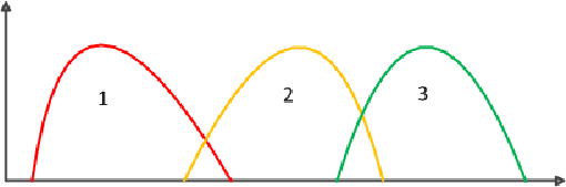
For example, assume $n$ linguistic constants are illustrated as the Fig. 1 shows. Based on the area of intersection $S_{ij}$ and union $U_{ij}$ between any two linguistic constants $L_{i}$ and $L_{j}$ , the non-exclusive degree $E_{ij}$ can be calculated to represent the non-exclusive degree between two D numbers.

Refer to caption — Figure 1: Example for linguistic constants

Definition 8.

Given an intersection matrix $\underline{\underline{I}}$ between two subsets belong to ${2^{\Omega}}$ . The intersection degree of two subsets, and the intersection degree can be defined as follows:

I({S_{1}},{S_{2}})=\frac{{\sum\limits_{i={S_{1}}(1)}^{\left|{{S_{1}}}\right|}{\sum\limits_{j={S_{2}}(1)}^{\left|{{S_{2}}}\right|}{{E_{ij}}}}}}{{\left|{{S_{1}}}\right|\cdot\left|{{S_{2}}}\right|}}

(17)

where $i\neq j$ , $S_{1},S_{2}\in{2^{\Omega}}$ . ${S_{1}}(1)$ represent the first element in the set $S_{1}$ , so do the set ${\left|{{S_{2}}}\right|}$ . ${\left|{{S_{1}}}\right|}$ denotes the cardinality of $S_{1}$ , and ${\left|{{S_{2}}}\right|}$ denotes the cardinality of $S_{2}$ . Note that, when $i=j$ , $I=1$ .

3.3 Distance between two D numbers

Since D numbers theory is a generalization of the Dempster-Shafer theory, a body of D numbers can be seen as a discrete random variable whose values are ${2^{\Omega}}$ with a probability distribution $d$ . Based on above, a D number is a vector $\vec{d}$ of the vector space. Thus, the distance between two D numbers is defined as follows.

Definition 9.

Let $d_{1}$ and $d_{2}$ be two D numbers on the same frame of discernment $\Omega$ , containing N elements which are not require to be exclusive with each other. The distance between $d_{1}$ and $d_{2}$ is:

d_{D-number({d_{1}},{d_{2}})}=\sqrt{\frac{1}{2}{{(\vec{{d_{1}}}-\vec{{d_{2}}})}^{T}}\underline{\underline{D}}{\cdot}\underline{\underline{I}}(\vec{{d_{1}}}-\vec{{d_{2}}})}

(18)

where ${\underline{\underline{D}}}$ and ${\underline{\underline{I}}}$ are two $({2^{\Omega}}\times{2^{\Omega}})$ -dimensional matrixes. The elements of ${\underline{\underline{D}}}$ are:

$D(A,B)=\frac{{\left|{{A}\cap{B}}\right|}}{{\left|{{A}\cup{B}}\right|}}$ . $(A,B\in{2^{\Omega}})$ .

The elements of ${\underline{\underline{I}}}$ are:

$I({A},{B})=\frac{{\sum\limits_{i={A}(1)}^{n}{\sum\limits_{j={B}(1)}^{m}{{E_{ij}}}}}}{{\left|{{A}}\right|\cdot\left|{{B}}\right|}}$ . $(i\neq j)$ , $(A,B\in{2^{\Omega}})$ , (when $i=j,I=1$ ).

An illustrative example is given to show the calculation of the distance between two D numbers step by step.

Example 2. Let $\Omega$ be a frame of discernment with 3 elements. We use 1,2,3 to denote element 1, element 2, and element 3 in the frame. The relationship of the three elements are shown in Fig. 2.

Given ${U_{12}}=2$ , ${U_{23}}=3$ , ${S_{12}}=0.2$ , ${S_{23}}=0.6$ . Two bodies of D numbers are given as follows:

${d_{1}}(\{1\})=0.3$ , ${d_{1}}(\{1,2\})=0.4$ , ${d_{1}}(\{1,2,3\})=0.4$ .

${d_{2}}(\{2\})=0.2$ , ${d_{2}}(\{2,3\})=0.3$ , ${d_{2}}(\{1,2,3\})=0.5$ .

Step 1 Constructing the vector $\vec{{d_{1}}}$ and $\vec{{d_{2}}}$ :

$\vec{{d_{1}}}=\left(\begin{array}[]{c}0.3\\ 0\\ 0\\ 0.4\\ 0.3\end{array}\right)$ , $\vec{{d_{2}}}=\left(\begin{array}[]{c}0\\ 0.2\\ 0.3\\ 0\\ 0.5\end{array}\right)$ .

${\vec{{d_{1}}}-\vec{{d_{2}}}}=\left(\begin{array}[]{c}0.3\\ -0.2\\ -0.3\\ 0.4\\ -0.2\end{array}\right)$

Step 2 Based on the given $U$ and $S$ , the relative matrix can be calculated as below:

$R=\left[\begin{array}[]{ccccccc}&1&2&3\\ 1&1&0.1&0\\ 2&0.1&1&0.2\\ 3&0&0.2&1\end{array}\right]$

Step 3 Calculate the distance matrix $\underline{\underline{D}}$ according to Eq. 9. For example, the distance between ${1}$ and ${1,2}$ can be calculated as follows:

$D(\{1\},\{1,2\})=\frac{{\left|{\{1\}}\right|}}{{\left|{\{1,2\}}\right|}}=\frac{1}{2}$

The distance matrix $\underline{\underline{D}}$ is:

$\underline{\underline{D}}=\left(\begin{array}[]{ccccccc}1&0&0&1/2&1/3\\ 0&1&0&1/2&1/3\\ 0&0&1&0&1/3\\ 1/2&1/2&0&1&2/3\\ 1/3&1/3&1/3&2/3&1\end{array}\right)$

Step 4 Calculate the intersection matrix $\underline{\underline{I}}$ according to Eq. 18. For example, the intersection degree between ${1,2}$ and ${1,2,3}$ can be calculated as follows:

$n={\left|{{S_{1}}}\right|}=2$ , $m={\left|{{S_{2}}}\right|}=3$ .

$I({S_{1}},{S_{2}})=\frac{{\sum\limits_{i={S_{1}}(1)}^{n}{\sum\limits_{j={S_{2}}(1)}^{m}{{E_{ij}}}}}}{{\left|{{S_{1}}}\right|\cdot\left|{{S_{2}}}\right|}}=\frac{{\sum\limits_{i=1}^{2}{\sum\limits_{j=1}^{3}{{E_{ij}}}}}}{{2\cdot 3}}=\frac{{0.1+0+0.1+0.2}}{6}=0.0667$

The intersection matrix is built as follows:

$\underline{\underline{I}}=\left(\begin{array}[]{ccccccc}1&0.1&0&0.05&0.0333\\ 0.1&1&0.2&0.05&0.1\\ 0&0.2&1&0.1&0.0667\\ 0.05&0.05&0.1&1&0.0667\\ 0.0333&0.1&0.0667&0.0667&1\end{array}\right)$

Step 5 Calculate the distance between the two D numbers according to Eq. 18.

$d_{D-number({d_{1}},{d_{2}})}=\sqrt{\frac{1}{2}{{(\vec{{d_{1}}}-\vec{{d_{2}}})}^{T}}\underline{\underline{D}}{\cdot}\underline{\underline{I}}(\vec{{d_{1}}}-\vec{{d_{2}}})}=0.4312$

4 Case study

In this section, some examples are given to study the discipline of distance between two D numbers. The following example shows the difference between $d_{BPA}$ and $d_{D-number}$ in an extreme situation.

Example 3. Let $\Omega$ be a frame of discernment with 2 linguistic constants, namely $\Omega=\{Good,Bad\}$ . The relationship between the two linguistic constants is shown in Fig. 3.

As the Fig. 3 shows, two constants are mutually exclusive. The distance function of D numbers is reasonable only if the discernment elements in the framework are not mutually exclusive, so we use the distance between two BPAs to calculate the distance of the two linguistic constants in Fig. 3.

Given two pairs of BPAs: ${m_{1}}(\{Good\})=1$ , ${m_{1}}(\{Bad\})=0$ ; ${m_{2}}(\{Good\})=0$ , ${m_{2}}(\{Bad\})=1$ .

The distance between the two BPAs can be calculated as bellow:

${d_{BPA}}=\sqrt{\frac{1}{2}(1,-1)\left(\begin{array}[]{c}1,0\\ 0,1\end{array}\right)\left(\begin{array}[]{c}1\\ -1\end{array}\right)}=1$

If the relationship between the two linguistic constants are shown in the Fig. 4, the two linguistic constants are not exclusive. The distance between two BPAs can not be used in this situation, so we use the proposed distance function of D numbers to calculate it.

Given two pairs of D numbers: ${d_{1}}(\{Good\})=1$ , ${d_{1}}(\{Bad\})=0$ ; ${d_{2}}(\{Good\})=0$ , ${d_{2}}(\{Bad\})=1$ .

Assume that the relationship between the two D numbers can be expressed as ${E_{12}}=0.2$ . The distance between the two D numbers can be calculated as bellow:

${d_{D-num({d_{1}},{d_{2}})}}=\sqrt{\frac{1}{2}\left({1,-1}\right)\left(\begin{array}[]{l}1,0\\ 0,1\end{array}\right)\left(\begin{array}[]{c}1,0.2\\ 0.2,1\end{array}\right)\left(\begin{array}[]{c}1\\ -1\end{array}\right)}=\sqrt{0.8}=0.8944$

From the example above, the proposed distance function of D numbers is reasonable when the discernment elements in the framework are not mutually exclusive. In the situation that the discernment is mutually exclusive, the proposed distance function of D numbers is degenerated as the distance function between two BPAs. This example proved that the proposed distance function based on D numbers is reasonable and effective. Another two examples are given to compare the difference between the $d_{BPA}$ and the $d_{D-number}$ as follows.

Example 4. Let $\Omega$ be a frame of discernment with 20 elements. We use 1,2,etc. to denote element 1, element 2, etc. The elements in the frame of discernment are exclusive between each other. In this situation, given two pairs of BPAs and D numbers as follows:

${m_{1}}(\{2,3,4\})=0.3$ , ${m_{1}}(\{7\})=0.4$ , ${m_{1}}(\{\Omega\})=0.4$ , ${m_{1}}(\{A\})=0.8$ .

${m_{2}}(\{1,2,3,4,5\})=1$ .

${d_{1}}(\{2,3,4\})=0.3$ , ${d_{1}}(\{7\})=0.4$ , ${d_{1}}(\{\Omega\})=0.4$ , ${d_{1}}(\{A\})=0.8$ .

${d_{2}}(\{1,2,3,4,5\})=1$ .

where $A$ is a subset of $\Omega$ .

The relative matrix can be calculated as below:

$R=\left[\begin{array}[]{ccccccc}&1&2&3&4&\ldots&20\\ 1&1&0&0&0&\ldots&0\\ 2&0&1&0&0&\ldots&0\\ 3&0&0&1&0&\ldots&0\\ 4&0&0&0&1&\ldots&0\\ \vdots&\vdots&\vdots&\vdots&\vdots&\vdots&\vdots\\ 20&0&0&0&0&\ldots&1\\ \end{array}\right]$

There are 20 cases where subset $A$ increments one or more element at a time, starting from Case 1 with $A={1}$ and ending with Case 20 when $A=\Omega$ . The distance between two BPAs $d_{BPA}$ defined in [56] and the distance between two D numbers $d_{D-number1}$ proposed in this paper in this condition are shown in the Table 1 and graphically illustrated in Fig. 5

The Fig. 5 shows that in the situation that the discernment is mutually exclusive, the proposed distance function of D numbers $d_{D-number1}$ is degenerated as the distance function between two BPAs $d_{BPA}$ .

Example 5. Let $\Omega$ be a frame of discernment with 20 elements. We use 1,2,etc. to denote element 1, element 2, etc. in the frame. The relationship between each two elements is shown in Fig. 6. In this case, let element 4 to element 20 be exclusive from each other, and given ${U_{12}}=2$ , ${U_{23}}=3$ , ${S_{12}}=0.2$ , ${S_{23}}=0.6$ .

Based on the given $U$ and $S$ , the relative matrix can be calculated as below:

$R=\left[\begin{array}[]{ccccccc}&1&2&3&4&\ldots&20\\ 1&1&0.1&0&0&\ldots&0\\ 2&0.1&1&0.2&0&\ldots&0\\ 3&0&0.2&1&0&\ldots&0\\ 4&0&0&0&1&\ldots&0\\ \vdots&\vdots&\vdots&\vdots&\vdots&\vdots&\vdots\\ 20&0&0&0&0&\ldots&1\\ \end{array}\right]$

The first D number ${d_{1}}$ is defined as

${d_{1}}(\{2,3,4\})=0.3$ , ${d_{1}}(\{7\})=0.4$ , ${d_{1}}(\{\Omega\})=0.4$ , ${d_{1}}(\{A\})=0.8$ .

where $A$ is a subset of $\Omega$ . The second D number ${d_{2}}$ used in the example is

${d_{2}}(\{1,2,3,4,5\})=1$ .

There are 20 cases where subset $A$ increments one or more element at a time, starting from Case 1 with $A={1}$ and ending with Case 20 when $A=\Omega$ as shown in Table 1. The distance between two D numbers $d_{D-number2}$ in this situation for these 20 cases is detailed in Table 1 and graphically illustrated in Fig. .

Table 1: Comparison of

d_{BPA}

and

d_{D-number}

values of

d_{1}

and

d_{2}

when subset

A

changes.

Cases	$d_{BPA}$	$d_{D-number1}$	$d_{D-number2}$
A = { 1}	0.7858	0.7858	0.7788
A = { 1,2}	0.6867	0.6867	0.6721
A = { 1,2,3}	0.5705	0.5705	0.5589
A = { 1,…,4}	0.4237	0.4237	0.4180
A = { 1,…,5}	0.1323	0.1323	0.1322
A = { 1,…,6}	0.3884	0.3884	0.3857
A = { 1,…,7}	0.5029	0.5029	0.4999
A = { 1,…,8}	0.5705	0.5705	0.5677
A = { 1,…,9}	0.6187	0.6187	0.6162
A = { 1,…,10}	0.6554	0.6554	0.6532
A = { 1,…,11}	0.6844	0.6844	0.6826
A = { 1,…,12}	0.7081	0.7081	0.7066
A = { 1,…,13}	0.7281	0.7281	0.7268
A = { 1,…,14}	0.7451	0.7451	0.7440
A = { 1,…,15}	0.7600	0.7600	0.7590
A = { 1,…,16}	0.7730	0.7730	0.7722
A = { 1,…,17}	0.7846	0.7846	0.7840
A = { 1,…,18}	0.7951	0.7951	0.7945
A = { 1,…,19}	0.8046	0.8046	0.8042
A = { 1,…,20}	0.8133	0.8133	0.8139

From the Table 1 and Fig. 7, both measures go up and down consistently, when the size of $A$ changes. However, the $d_{D-number}$ values are always little smaller than the corresponding $d_{BPA}$ values, because the elements in set $\Omega$ do not require mutually exclusive in D numbers. The Example 4 and Example 5 proved that the proposed distance function of D numbers is effective when the elements in the frame of discernment are not mutually exclusive. When the discernment is mutually exclusive, the distance function of D numbers is degenerated as the distance function between two BPAs defined by Anne-Laure Jousselme.

5 Conclusion

In this paper, a new distance function to measure the distance between two D numbers is proposed. D number is a new representation of uncertain information, which inherits the advantage of the Dempster-Shafer theory of evidence and overcomes some shortcomings. The proposed distance function of D numbers is effective when the elements in the frame of discernment are not mutually exclusive. In the situation that the elements in the frame of discernment are mutually exclusive, the proposed distance function of D numbers is degenerated as the distance function between two BPAs defined by Anne-Laure Jousselme.

Acknowledgements

The work is partially supported by National Natural Science Foundation of China (Grant No. 61174022), Specialized Research Fund for the Doctoral Program of Higher Education (Grant No. 20131102130002), R&D Program of China (2012BAH07B01), National High Technology Research and Development Program of China (863 Program) (Grant No. 2013AA013801), the open funding project of State Key Laboratory of Virtual Reality Technology and Systems, Beihang University (Grant No.BUAA-VR-14KF-02).

References

[1] A. P. Dempster, Upper and lower probabilities induced by a multivalued mapping, The annals of mathematical statistics 38 (2) (1967) 325–339.
[2] G. Shafer, A mathematical theory of evidence, Vol. 1, Princeton university press Princeton, 1976.
[3] A. P. Dempster, A generalization of bayesian inference, Tech. rep., DTIC Document (1967).
[4] I. Bloch, Some aspects of dempster-shafer evidence theory for classification of multi-modality medical images taking partial volume effect into account, Pattern Recognition Letters 17 (8) (1996) 905–919.
[5] R. P. Srivastava, L. Liu, Applications of belief functions in business decisions: A review, Information Systems Frontiers 5 (4) (2003) 359–378.
[6] F. Cuzzolin, A geometric approach to the theory of evidence, Systems, Man, and Cybernetics, Part C: Applications and Reviews, IEEE Transactions on 38 (4) (2008) 522–534.
[7] M.-H. Masson, T. Denoeux, Ecm: An evidential version of the fuzzy c-means algorithm, Pattern Recognition 41 (4) (2008) 1384–1397.
[8] T. Denœux, Maximum likelihood estimation from fuzzy data using the em algorithm, Fuzzy sets and systems 183 (1) (2011) 72–91.
[9] Y. Deng, R. Sadiq, W. Jiang, S. Tesfamariam, Risk analysis in a linguistic environment: a fuzzy evidential reasoning-based approach, Expert Systems with Applications 38 (2011) 15438–15446.
[10] Y. Deng, W. Jiang, R. Sadiq, Modeling contaminant intrusion in water distribution networks: A new similarity-based dst method, Expert Systems with Applications 38 (2011) 571–578.
[11] Y. Deng, F. T. Chan, A new fuzzy dempster mcdm method and its application in supplier selection, Expert Systems with Applications 38 (2011) 9854–9861.
[12] Y. Zhang, X. Deng, D. Wei, Y. Deng, Assessment of e-commerce security using ahp and evidential reasoning, Expert Systems with Applications 39 (2012) 3611–3623.
[13] B. Kang, Y. Deng, R. Sadiq, S. Mahadevan, Evidential cognitive maps, Knowledge-Based Systems.
[14] T. Denoeux, Maximum likelihood estimation from uncertain data in the belief function framework, Knowledge and Data Engineering, IEEE Transactions on 25 (1) (2013) 119–130.
[15] Y. Yang, D. Han, C. Han, Discounted combination of unreliable evidence using degree of disagreement, International Journal of Approximate Reasoning 54 (8) (2013) 1197–1216.
[16] Y. Yang, D. Han, C. Han, F. Cao, A novel approximation of basic probability assignment based on rank-level fusion, Chinese Journal of Aeronautics 26 (4) (2013) 993–999.
[17] D. Wei, X. Deng, X. Zhang, Y. Deng, S. Mahadevan, Identifying influential nodes in weighted networks based on evidence theory, Physica A: Statistical Mechanics and its Applications 392 (10) (2013) 2564–2575.
[18] Z.-g. Liu, Q. Pan, J. Dezert, Evidential classifier for imprecise data based on belief functions, Knowledge-Based Systems 52 (2013) 246–257.
[19] X. Deng, Y. Hu, Y. Deng, S. Mahadevan, Supplier selection using ahp methodology extended by d numbers, Expert Systems with Applications 41 (1) (2014) 156–167.
[20] R. R. Yager, On the aggregation of prioritized belief structures, Systems, Man and Cybernetics, Part A: Systems and Humans, IEEE Transactions on 26 (6) (1996) 708–717.
[21] J. Gebhardt, R. Kruse, Parallel combination of information sources, in: Belief Change, Springer, 1998, pp. 393–439.
[22] E. Lefèvre, Z. Elouedi, How to preserve the conflict as an alarm in the combination of belief functions?, Decision Support Systems 56 (2013) 326–333.
[23] J.-B. Yang, D.-L. Xu, Evidential reasoning rule for evidence combination, Artificial Intelligence 205 (2013) 1–29.
[24] R. R. Yager, On the dempster-shafer framework and new combination rules, Information sciences 41 (2) (1987) 93–137.
[25] E. Lefevre, O. Colot, P. Vannoorenberghe, Belief function combination and conflict management, Information fusion 3 (2) (2002) 149–162.
[26] W. Liu, Analyzing the degree of conflict among belief functions, Artificial Intelligence 170 (11) (2006) 909–924.
[27] J. Schubert, Conflict management in dempster–shafer theory using the degree of falsity, International Journal of Approximate Reasoning 52 (3) (2011) 449–460.
[28] A. Tchamova, J. Dezert, On the behavior of dempster’s rule of combination and the foundations of dempster-shafer theory, in: Intelligent Systems (IS), 2012 6th IEEE International Conference, IEEE, 2012, pp. 108–113.
[29] N. Bastian, K. R. Covey, M. R. Meyer, A universal stellar initial mass function? a critical look at variations, arXiv preprint arXiv:1001.2965.
[30] M. Cappellari, R. M. McDermid, K. Alatalo, L. Blitz, M. Bois, F. Bournaud, M. Bureau, A. F. Crocker, R. L. Davies, T. A. Davis, et al., Systematic variation of the stellar initial mass function in early-type galaxies, Nature 484 (7395) (2012) 485–488.
[31] Z.-g. Liu, Q. Pan, J. Dezert, A belief classification rule for imprecise data, Applied Intelligence (2013) 1–15.
[32] P. Xu, Y. Deng, X. Su, S. Mahadevan, A new method to determine basic probability assignment from training data, Knowledge-Based Systems 46 (2013) 69–80.
[33] T. Burger, S. Destercke, How to randomly generate mass functions, International Journal of Uncertainty, Fuzziness and Knowledge-Based Systems 21 (05) (2013) 645–673.
[34] Z.-g. Liu, Q. Pan, J. Dezert, G. Mercier, Credal classification rule for uncertain data based on belief functions, Pattern Recognition 47 (7) (2014) 2532–2541.
[35] G. J. Klir, Generalized information theory, Fuzzy sets and systems 40 (1) (1991) 127–142.
[36] R. Bachmann, S. Elstner, E. R. Sims, Uncertainty and economic activity: Evidence from business survey data, Tech. rep., National Bureau of Economic Research (2010).
[37] A. Bronevich, G. J. Klir, Measures of uncertainty for imprecise probabilities: An axiomatic approach, International journal of approximate reasoning 51 (4) (2010) 365–390.
[38] S. R. Baker, N. Bloom, S. J. Davis, Measuring economic policy uncertainty, policyuncertainy. com.
[39] I. Couso, S. Moral, Independence concepts in evidence theory, International Journal of Approximate Reasoning 51 (7) (2010) 748–758.
[40] P. Limbourg, E. De Rocquigny, Uncertainty analysis using evidence theory–confronting level-1 and level-2 approaches with data availability and computational constraints, Reliability Engineering & System Safety 95 (5) (2010) 550–564.
[41] R. Jiroušek, J. Vejnarová, Compositional models and conditional independence in evidence theory, International Journal of Approximate Reasoning 52 (3) (2011) 316–334.
[42] H. Luo, S.-l. Yang, X.-j. Hu, X.-x. Hu, Agent oriented intelligent fault diagnosis system using evidence theory, Expert Systems with Applications 39 (3) (2012) 2524–2531.
[43] F. Karahan, S. Ozkan, On the persistence of income shocks over the life cycle: Evidence, theory, and implications, Review of Economic Dynamics 16 (3) (2013) 452–476.
[44] S. Mao, Z. Zou, Y. Xue, Y. Li, A model based on the coupled rules of evidence theory used in multiple objective decisions, in: 2014 International Conference on Global Economy, Finance and Humanities Research (GEFHR 2014), Atlantis Press, 2014.
[45] Z. Zhang, C. Jiang, X. Han, D. Hu, S. Yu, A response surface approach for structural reliability analysis using evidence theory, Advances in Engineering Software 69 (2014) 37–45.
[46] J. Liu, F. T. Chan, Y. Li, Y. Zhang, Y. Deng, A new optimal consensus method with minimum cost in fuzzy group decision, Knowledge-Based Systems 35 (2012) 357–360.
[47] X. Zhang, Y. Deng, F. T. Chan, P. Xu, S. Mahadevan, Y. Hu, Ifsjsp: A novel methodology for the job-shop scheduling problem based on intuitionistic fuzzy sets, International Journal of Production Research 51 (17) (2013) 5100–5119.
[48] Y. Deng, D numbers: Theory and applications, Journal of Information and Computational Science 9 (9) (2012) 2421–2428.
[49] X. Deng, Y. Hu, Y. Deng, S. Mahadevan, Environmental impact assessment based on D numbers, Expert Systems with Applications 41 (2) (2014) 635–643.
[50] X. Deng, Y. Hu, Y. Deng, S. Mahadevan, Supplier selection using AHP methodology extended by D numbers, Expert Systems with Applications 41 (1) (2014) 156–167.
[51] X. Deng, Y. Hu, Y. Deng, Bridge condition assessment using D numbers, The Scientific World Journal 2014 (2014) Article ID 358057, 11 pages. doi:10.1155/2014/358057.
[52] X. Deng, F. T. Chan, R. Sadiq, S. Mahadevan, Y. Deng, D-cfpr: D numbers extended consistent fuzzy preference relations, arXiv preprint arXiv:1403.5753.
[53] B. Tessem, et al., Approximations for efficient computation in the theory of evidence, Artificial Intelligence 61 (2) (1993) 315–329.
[54] L. M. Zouhal, T. Denœux, An evidence-theoretic k-nn rule with parameter optimization, Systems, Man, and Cybernetics, Part C: Applications and Reviews, IEEE Transactions on 28 (2) (1998) 263–271.
[55] M. Bauer, Approximation algorithms and decision making in the dempster-shafer theory of evidence¡ªan empirical study, International Journal of Approximate Reasoning 17 (2) (1997) 217–237.
[56] A.-L. Jousselme, D. Grenier, É. Bossé, A new distance between two bodies of evidence, Information fusion 2 (2) (2001) 91–101.
[57] A.-L. Jousselme, P. Maupin, Distances in evidence theory: Comprehensive survey and generalizations, International Journal of Approximate Reasoning 53 (2) (2012) 118–145.
[58] S. Huang, X. Su, Y. Hu, S. Mahadevan, Y. Deng, A new decision-making method by incomplete preferences based on evidence distance, Knowledge-Based Systems 56 (2013) 264¨C272.