A Floer Fundamental group
Groupe fondamental de Floer

In many ways, the topology of a space influences its geometry, and this is particularly true in symplectic geometry. Having a symplectic interpretation of a topological invariant is a good tool to explore this relationship. The celebrated Floer Homology ([9][10]) is of course a strong illustration of this phenomenon. Introduced to prove the homological version of the Arnold conjecture ([1]), it quickly became one of the most powerful tools in symplectic geometry.

However, all the techniques derived from the original Floer construction are homological, or at least chain complex based in nature. The notion of cobordism (among moduli spaces) is even at the root of the original ideas of M. Gromov [12] of using pseudo-holomorphic curves to derive invariants in symplectic geometry. The use of local coefficients in Floer complexes allows Floer theory to involve some homotopical invariants, but purely homotopical tools are still missing, and it is the goal of this paper to provide a Floer theoretic interpretation of the fundamental group.

All the objects this construction is based on are still classical Floer theoretic objects, but the essential non Abelian phenomena that make the difference between the fundamental group and the first homology group are caught by a deeper use of $1$-dimensional moduli spaces, and the use of “augmentations”.

More precisely, let $(M,\omega)$ be a connected closed monotone symplectic manifold and choose an Hamiltonian function $H$ on $M$, a possibly time dependent almost complex structure $J$ compatible with $\omega$, and a point $\star$ in $M$ to serve as the base point. Recall the Floer trajectories in this setting are (finite energy) maps $u:\mathbb{R}\times S^{1}\to M$ satisfying the Floer equation

where $X_{H}$ is the Hamiltonian vector field associated to $H$.

Using a cutoff function $\chi$ to turn off the non homogeneous Hamiltonian term on the positive end of the tube (resp. on both ends but preserving it on an annulus of varying modulus) allows to define moduli spaces denoted by $\mathcal{M}(x,\varnothing)$ (resp. $\mathcal{M}(\star,\varnothing)$), which are Floer counterparts of Morse unstable manifolds (see the comments after definition 2.4). It is a classical result of Floer theory that for a generic set of auxiliary data $(H,J,\star,\chi)$, all these moduli spaces are smooth finite dimensional manifolds.

Similarly to the Morse setting where a loop can be seen as a concatenation of paths associated to unstable manifolds of index $1$ critical points, we use the components of the above $1$-dimensional moduli spaces to define a notion of Floer loop (see definition 2.8). These loops come naturally with concatenation and cancellation relations for which they form a group ${\mathcal{L}(H,\star)}$. The main statement of the paper is then the following theorem :

A description of the relations is also given, but, although they obviously only depend on $H$, $J$, $\star$, and $\chi$, we resort to an auxiliary Morse function to get a finite presentation for them (see section 4). Nevertheless, we produce explicit relations such that the generated normal subgroup ${\mathcal{R}(H,\star)}$ satisfies the following statement :

Notice the construction is presented here in the absolute setting, i.e. Hamiltonian fixed points problem, but also makes sense in the relative one, i.e. intersections of a Lagrangian sub-manifold with its deformations under Hamiltonian isotopies problem. Although the latter can be expected to hold the most interesting applications, we choose to focus on the former for the sake of simplicity and to better highlight the main ideas : the generalization to the latter entails exactly the same issues as for the homology and involves no new idea.

Finally, the construction also makes sense in the stable Morse setting (i.e. study of Morse functions that are quadratic at infinity on $M\times\mathbb{R}^{N}$). Although the corresponding results have their own interest and would deserve a separate discussion, they will only be quickly sketched without proofs in the last section of this paper (see section 6), rather as an illustration and a simplified finite dimensional model of the Floer setting.

A natural outcome of this construction is an estimate on the number of fixed points of Hamiltonian diffeomorphisms, but not in usual way, since a notion of multiplicity has to be introduced. Indeed, rather than the critical points themselves, the relevant objects required to build loops are their unstable manifolds (called “steps” in the sequel), and while to one critical point corresponds exactly one unstable manifold in the Morse setting, Floer counterparts of unstable manifolds may have several components, which have all to be taken into account.

Counting the number $\nu_{J}(x)$ (resp. $\nu_{J}(\star)$) of steps through a given Conley-Zehnder index $1-n$ fixed point $x$ (resp. $\star$) defines a notion of multiplicity for these points (that depends on the almost complex structure, see definition 2.10 for more details). We then have the following theorem :

The role and the control of the contributions of the multiplicities in general is a deep and intriguing question, closely related to the estimation of the minimal number of periodic orbits.

The following theorem ensures the existence of at least one Hamiltonian periodic orbit with Conley-Zehnder index $1-n$ and non vanishing multiplicity provided the fundamental group is non trivial :

In particular, this result provides at least one index $1-n$ orbit even if the first homology group of the manifold vanishes, provided the fundamental group is non trivial.

One interesting feature of this theorem is that its proof is essentially geometric, where the usual Floer technics are rather algebraic : it comes down to patching suspensions of $1$-dimensional moduli spaces side to side to form a disc. In this sense, although theorem 1.4 is not strictly speaking a corollary of the Floer interpretation of the fundamental group given in this paper, it derives from the same principal idea, namely that $1$-dimensional moduli spaces do contain information that the homology does not catch.

Moreover, the orbit exhibited in this statement has explicitly non vanishing multiplicity, while this is not immediately obvious in other constructions that provide lower bounds on the number of periodic orbits.

Theorem 1.3 is obviously a variation on the Arnold conjecture. In its non degenerate and strongest form, this conjecture claims that the total number of $1$-periodic orbits of a non degenerate Hamiltonian flow can not be less than the minimal number of critical points for a Morse function (or stable Morse function in a weaker form of the conjecture). A weaker but maybe more convincing and tractable version involves the stable Morse number, which is the minimal number of critical points of Morse functions which are quadratic at infinity on products $M\times\mathbb{R}^{N}$.

This conjecture is closely related to the birth of symplectic geometry itself. A strong breakthrough was achieved by A. Floer who constructed his chain complex to establish the Homological version of the Arnold conjecture for compact monotone symplectic manifolds, opening the way to huge efforts by many authors to generalize his original construction.

Until very recently however, work regarding this conjecture was focused on its homological version.

In a recent work [15], K. Ono and A. Pajitnov use the Floer complex with local coefficients to extend these constraints to the Hamiltonian setting. In particular, they show the following

Similarly to the stable Morse setting, the points of view of this theorem and theorem 1.3 are essentially different : the former focuses on the number of geometric fixed points, while the latter associates possibly several generators to the same geometric orbit to overcome an eventual lack of generators and still recover the fundamental group.

In the second section of the paper (the first is this introduction), the main definitions, statements and technical tools are presented. The third section is dedicated to the comparison of Morse and Floer loops, and the proof of theorem 1.1. The fourth section is devoted to the description of the relations, and the fifth to the proof of the application (theorem 1.3) and theorem 1.4. Finally, the last section is a sketch without proofs of the construction in the Stable Morse setting.

This work would not exist without the crucial help of a few people. I am particularly thankful to O. Cornea, whose deep topological insight and generosity nourished me for years, to J.-Y. Welschinger and B. Chantraine to whom I am indebted for the keystone of this paper, which is the notion of augmentation, to A. Oancea who served as a compass to me and to M. Damian who also owns a large part of this work. Finally, I’m particularly grateful to A.V. Duffrène who indirectly but deeply influenced the birth of this paper.

Let $(M,\omega)$ be a $2n$-dimensional connected compact symplectic manifold without boundary. For technical reasons, $M$ will be supposed to be either

• •

  symplectically aspherical, which means $\omega$ vanishes on the image of the Hurewicz homomorphism $\pi_{2}(M)\to H_{2}(M)$, or

• •

  monotone, which means $c_{1}(TM)$ and $\omega$ are proportional by a positive constant on the image of the Hurewicz homomorphism $\pi_{2}(M)\to H_{2}(M)$.

These assumptions will allow us to easily

• •

  avoid the transversality issues related to the multiply covered negative curves,

• •

  avoid bubbles on $0$ and $1$-dimensional moduli spaces,

• •

  ensure finiteness of the number of (lifted) orbits of given Conley-Zehnder index.

Given a Hamiltonian function $H:M\times\mathbb{S}^{1}\to\mathbb{R}$, we let $X_{H}$ be the associated Hamiltonian vector field, $\phi^{t}_{H}$ its flow, and $\mathcal{P}(H)$ the set of its contractible $1$-periodic orbits.

To handle the index computation when $c_{1}(TM)$ does not vanish on $\pi_{2}(M)$, we consider the covering $\tilde{\mathcal{P}}(H)$ associated to the group $\pi_{2}(M)/\ker c_{1}$. It is obtained from $\mathcal{P}(H)$ by adjoining a capping class to the orbit in the following way :

where $D$ is the $2$-disc and $(\gamma,\bar{\gamma})\sim(\gamma^{\prime},\bar{\gamma}^{\prime})$ iff $\gamma=\gamma^{\prime}$ and $\mu_{CZ}(\bar{\gamma})=\mu_{CZ}(\bar{\gamma}^{\prime})$ ($\mu_{CZ}$ denoting the Conley-Zehnder index).

Notice that this last equality implies that the two cappings also have the same symplectic area : glued along their boundary, $\bar{\gamma}$ and $\bar{\gamma}^{\prime}$ with the reversed orientation form a sphere $S$ with vanishing first Chern class, and because of our asphericity or monotonicity assumption, $\iint_{S}\omega=0$, which means that $\bar{\gamma}$ and $\bar{\gamma}^{\prime}$ have the same symplectic area. As a consequence, both the Conley-Zehnder index and the symplectic area are well defined for equivalence classes of cappings.

In the sequel, $\tilde{\mathcal{P}}(H)$ will completely replace $\mathcal{P}(H)$ and no explicit reference to the covering will be made anymore. In particular, what we call a Hamiltonian orbit from now on will in fact be a lift of such an orbit to $\tilde{\mathcal{P}}(H)$.

Each element $x$ in $\tilde{\mathcal{P}}(H)$ then has a well defined Conley-Zehnder index $\mu_{CZ}$. For convenience, we shift the Conley-Zehnder index by $n$ and let

The set of orbits $\tilde{\mathcal{P}}(H)$ splits according to this index, and we let

Given a (possibly time dependent) $\omega$-compatible almost complex structure $J$, we are interested in the Floer moduli spaces and some classical variants of such that we describe below. Recall the Floer equation for a map $u:\mathbb{R}\times\mathbb{S}^{1}\to M$ is the following :

Moreover, we fix once for all a smooth function $\chi:\mathbb{R}\to[0,1]$ such that

and use it to cutoff the Hamiltonian term of the Floer equation on one or both ends of the cylinder by considering the equation

for different functions $\chi_{i}:\mathbb{R}\to[0,1]$, $i=1,2,3$ and $i=(4,R)$, derived from $\chi$, namely (see figure 1)

1. (1)

   $\chi_{1}\equiv 1$ defines the usual Floer equation,

2. (2)

   $\chi_{2}(s)=\chi(s)$ defines the “lower capping equation”,

3. (3)

   $\chi_{3}(s)=\chi(-s)$ defines the “upper capping equation”,

4. (4)

   $\chi_{4,R}(s)=\chi(s-R)\chi(-s-R)$ defines “$R$-perturbed sphere equation”.

In ($F_{4,R}$), $R$ is a real parameter, but notice that for $R\leq 0$, the equation has no Hamiltonian term anymore and does not depend on $R$ : $R$ will hence be considered in $[0,+\infty)$.

Recall that the energy of a solution $u$ of this equation is defined as

where $\|.\|_{t}=\omega(.,J_{t}.)$. Solutions of finite energy of this equation have converging ends, either to a point by the classical removal of singularities argument ([2],[13]) if the Hamiltonian term is cut off on this end, or to a Hamiltonian orbit if not ([8]). In the former case, considering the end as a neighborhood of $0$ in $\mathbb{C}\setminus\{0\}$, the map $u$ extends holomorphically through $0$, and the equations $(F_{i})$ above could equivalently be considered as defined on the sphere $\mathbb{CP}^{1}$ with $2$, $1$ or no puncture (see for instance [14] for a more uniform description of these equation, or [13] chapter 8 for the case without punctures, i.e. equation $(F_{4,R})$ with fixed $R$). Anyway, on an end where the Hamiltonian term is cut off, the limit value will be denoted by $u(+\infty)$ or $u(-\infty)$. We abusively but conveniently write that such a trajectory ends at the $\varnothing$ symbol to describe the fact that this limit point is not constrained.

We are interested in the moduli spaces described below and depicted on figure 2. Let $\star$ be a point in $M$, and $\mathcal{U}$ be the space of smooth maps $u:\mathbb{R}\times\mathbb{S}^{1}\to M$ that have finite energy i.e. such that $\iint\|\frac{\partial u}{\partial s}\|^{2}dsdt<+\infty$. If $a$ is an oriented disc, let $\bar{a}$ denote the disc with opposite orientation, and if $b$ is another disc or tube having the same boundary as $a$ , let $\bar{a}\sharp b$ denote the gluing of the two.

where the brackets denote classes in $\pi_{2}(M)/\ker c_{1}$, and their vanishing expresses the compatibility of the trajectory $u$ with the prescribed lifts of its ends to the covering space $\tilde{\mathcal{P}}(H)$.

Notice that in the last case, the parameter $R$ is allowed to vary, and that the moduli space $\overset{\ \circ}{\mathcal{M}}(\star,\varnothing)$ is endowed with the map $\overset{\ \circ}{\mathcal{M}}(\star,\varnothing)\xrightarrow{\pi}[0,+\infty)$ given by $\pi(u,R)=R$.

The three last types of moduli spaces are used in [16] (in conjunction with a Morse function that we do not use here) to define the PSS homomorphisms and compare Morse and Floer homologies.

Since the elements of $\overset{\ \circ}{\mathcal{M}}(x,\varnothing)$ for $x\in\tilde{\mathcal{P}}_{0}(H)$ can be used to define an augmentation on the Floer complex, we use the following terminology :

It is well known (see remark 5 below) that for a generic choice of $(H,J,\star,\chi)$, these moduli spaces are smooth manifolds whose dimension is prescribed by the end constraints and the homotopy class of the tube.

In particular, under a generic choice of $(H,J,\star,\chi)$, we have  :

From now on, $(H,J,\star,\chi)$ will be supposed to be chosen so that all these moduli spaces are indeed cut out transversely.

Moreover, all these moduli spaces are compact up to breaking or bubbling off of spheres, and we let

be the Gromov-Floer compactifications of the previous moduli spaces.

In all this paper, only $0$ and $1$-dimensional moduli spaces will be considered, and no bubbling of sphere can occur on such moduli spaces. This means they will all be compact up to breaking and smooth.

In particular, each $0$-dimensional moduli space $\mathcal{M}(y,x)$ is compact, and hence finite, and we let

denote the cardinality of $M(y,x)$.

Given a configuration of two consecutive isolated Floer trajectories $(\beta,\alpha)\in\mathcal{M}(y,x)\times\mathcal{M}(x,\varnothing)$ with $x\in\tilde{\mathcal{P}}_{0}(H)$ and $y\in\tilde{\mathcal{P}}_{1}(H)\cup\{\star\}$, the gluing construction ([10], [13]) gives rise to a one dimensional family of trajectories starting with $(\beta,\alpha)$ and ending at some other broken configuration $(\beta^{\prime},\alpha^{\prime})\in\mathcal{M}(y,x^{\prime})\times\mathcal{M}(x^{\prime},\varnothing)$. This relation between $(\beta,\alpha)$ and $(\beta^{\prime},\alpha^{\prime})$ will be denoted by

This “move” from one end of a moduli space to another described above in $\mathcal{M}(y,\varnothing)$ makes sense for all kinds of configurations, and will be the main ingredient of all the subsequent constructions. It therefore deserves a general definition :

Depending on the type of moduli space under consideration, there are several types of Floer steps. Floer loops will be built out of special steps, called Floer loop steps, which are depicted on figure 4 and specified in the following definition :

This somewhat abstruse definition is the heart of the construction and deserves some comments.

An enlightening point of view is that of Morse theory. Consider a function $f$ and a Riemannian metric $g$ on a manifold $M$ such that the pair $(f,g)$ is Morse-Smale. Starting with any generic loop in the manifold and pushing it down by the flow of $f$ deforms it into the concatenation of elementary paths, called “Morse steps”, that consist in travelling once, in one or the other direction, along the unstable manifold of an index $1$ critical point.

It turns out that these steps can be interpreted from the moduli space point of view : let $y$ be an index $1$ critical point and $W^{u}(y)$ its unstable manifold. To a point $p$ in the unstable manifold is associated a path, namely the piece of Morse trajectory from $y$ to $p$, and there is a one to one correspondence between such trajectory pieces and the unstable manifold (see [3] for a detailed presentation of this point of view, and a nice compactification of the unstable manifold derived from it). More precisely, define an “interrupted” Morse trajectory as a solution of the following modified Morse equation

where the cutoff function $\chi$ is the same as the one used in ($F_{2}$), i.e. a smooth decreasing function such that $\chi(s)=1$ for $s\leq-1$ and $\chi(s)=0$ for $s\geq 0$.

Using the same notation as in the Floer setting, let

This space is naturally endowed with an evaluation map (recall the trajectories are constant for $s\geq 0$ so $\gamma(+\infty)=\gamma(0)$),

which is one to one and provides an identification between $\overset{\ \circ}{\mathcal{M}}_{\mathrm{Morse}}(y,\varnothing)$ and $W^{u}(y)$.

Moreover, $\overset{\ \circ}{\mathcal{M}}_{\mathrm{Morse}}(y,\varnothing)$ has a natural compactification $\mathcal{M}_{\mathrm{Morse}}(y,\varnothing)$ as a $1$-dimensional segment whose ends are the two “broken” configurations $(\gamma_{\pm},\bar{x}_{\pm})$ where

• •

  $\gamma_{+}$ and $\gamma_{-}$ are the two Morse trajectories rooted at $y$,

• •

  $x_{\pm}$ is the index $0$ critical point such that $x_{\pm}=\lim_{s\to+\infty}\gamma_{\pm}$,

• •

  $\bar{x}_{\pm}$ is the constant solution of (12) at $x_{\pm}$. It is the one and only one augmentation of $x_{\pm}$.

The evaluation map extends to this compactification and defines a path running along $W^{u}(y)$ from $x_{-}$ to $x_{+}$, which is the “Morse loop step” associated to $y$.

From this point of view, a Floer loop step through an index $1$ periodic orbit is the exact counterpart of a Morse loop step through an index 1 critical point.

Similarly, assuming by genericity that $\star$ is not critical for $f$, the Morse counterpart of the space $\mathcal{M}(\star,\varnothing)$ is the collection of segments of the (unique) trajectory passing through $\star$, running from $\star$ down to some arbitrary point $p$ below it along this trajectory. It is in one to one correspondence with (the closure of) the piece of trajectory flowing from $\star$ down to the index $0$ critical point below it.

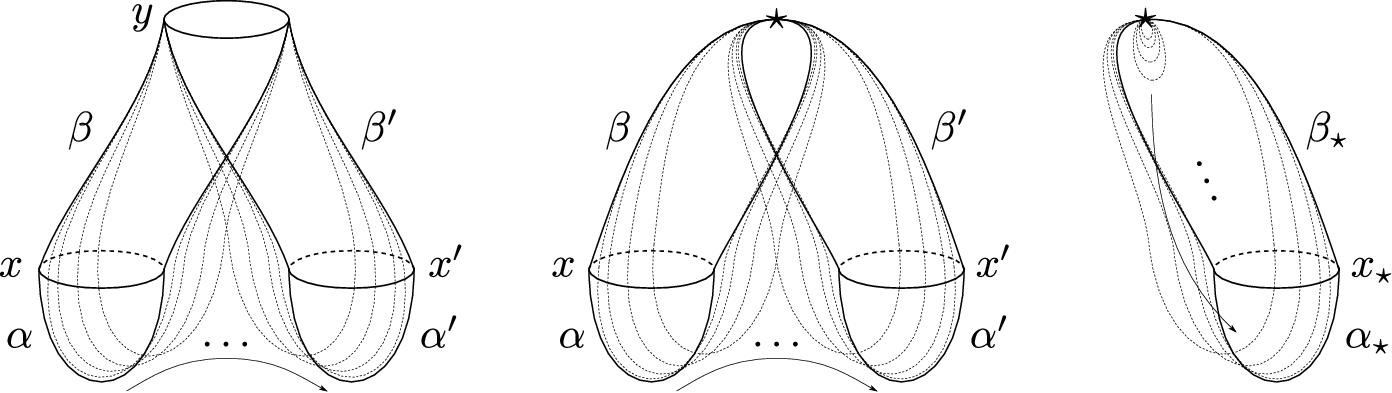
Definitions 2.3 and 2.4 are not very explicit and a more usable description of a step is obtained by specifying its ends :

The situation of Floer loop steps through $\star$ is slightly different, as there is one special step that does not look like the others.

Recall that the moduli space $\overset{\ \circ}{\mathcal{M}}(\star,\varnothing)$ comes with a projection to the non negative reals

This projection is proper, and extends continuously to a map $\mathcal{M}(\star,\varnothing)\xrightarrow{\pi}[0,+\infty]$ where all the broken configurations lie above $R=+\infty$. Moreover, the gluing construction ensures that exactly one component of $\mathcal{M}(\star,\varnothing)$ ends at each broken configuration.

Observe now that the same holds over $R=0$ : exactly one component of $\mathcal{M}(\star,\varnothing)$ ends at the constant map $(u_{\star},0)$. This is a direct consequence of the regularity of this solution stressed in proposition 2.2 (surjectivity of $L$ implies that $\pi:\mathcal{M}(\star,\varnothing)\to\mathbb{R}$ is a submersion at $(u_{\star},0)$).

As a consequence, $\mathcal{M}(\star,\varnothing)$ has exactly one connected component that relates $\{\star\}$ to a broken configuration, and all the other components either have no boundary or relate two broken configurations :

Notice finally that Floer loop steps are oriented and hence have a start and an end :

In other words, a Floer based loop is a sequence

Let ${\tilde{\mathcal{L}}(H,\star)}$ be the set of all Floer based loops. Notice it depends on all the auxiliary data $(H,\star,J,\chi)$ but the dependency on $J$ and $\chi$ is kept implicit to reduce the notation. It carries an obvious concatenation rule that turns it into a semi-group.

It also carries obvious cancellation rules. More explicitly, if $\sigma=(\alpha,\beta,\beta^{\prime},\alpha^{\prime})$ is a Floer loop step, define its inverse $\sigma^{-1}$ to be the same step with the opposite orientation :

Denote by $\sim$ the associated cancellation rules in ${\tilde{\mathcal{L}}(H,\star)}$ :

The concatenation then endows the quotient space

with a group structure.

A Floer loop step being a one parameter family of tubes, evaluation at the $+\infty$ end of the tube defines a path in $M$ (an arbitrary parameterization can be chosen for each step, since we are only interested in the resulting homotopy class), and induces a map

This map is compatible with both the concatenation and the cancellation rules and hence induces a group homomorphism

All the objects involved in theorem 1.1 are now defined and we recall its statement :

The description of the relations still requires the introduction of further technical ingredients, and we postpone it to section 4 to focus in the next section on the application to the count, with multiplicity, of Hamiltonian periodic orbits, since it only requires the surjectivity.

Notice the counting here is not algebraic but geometric : it is not hard to see that the algebraic count would always be $0$.

The following statement is a reformulation of theorem 1.3 and is a direct corollary of our construction. It will be proven in section 5.1.

References

- [1] V.I. Arnold, Méthodes mathématiques de la mécanique classique, Mir, Moscou, 1976.
- [2] M. Audin & F. Lafontaine, ed., Holomorphic curves in symplectic geometry. Progress in Mathematics 117, Birkhäuser 1994.
- [3] J.-F. Barraud & O. Cornea, Lagrangian intersections and the Serre spectral sequence. Ann. of Math. (2) 166 (2007), no. 3, 657–722.
- [4] P. Biran & O. Cornea, Lagrangian topology and enumerative geometry. Geom. Topol. 16 (2012), no. 2, 963–1052.
- [5] M. Damian, On the stable Morse number of a closed manifold. Bull. London Math. Soc. 34 (2002), no. 4, 420–430.
- [6] A. Floer, Cuplength estimates on Lagrangian intersections, Comm. Pure Appl. Math. 42 (1989), no. 4, 335–356.
- [7] A. Floer, Morse theory for Lagrangian intersections, J. Differential Geom. 28 (1988), no. 3, 513–547.
- [8] A. Floer, The unregularized gradient flow of the symplectic action, Comm. Pure Appl. Math. 41 (1988), no. 6, 775–813.
- [9] A. Floer, Witten’s complex and infinite-dimensional Morse theory, J. Differential Geom. 30 (1989), no. 1, 207–221.
- [10] A. Floer, Symplectic fixed points and holomorphic spheres, Commun. Math. Phys. 120 (1989), 575–611.
- [11] A. Floer, H. Hofer, D. Salamon, Transversality in elliptic Morse theory for the symplectic action, Duke Math. J. 80 (1995), no. 1, 251–292.
- [12] M. Gromov, Pseudo-holomorphic curves in symplectic manifolds, Invent. Math. 82 (1985), p. 307–347.
- [13] D. McDuff & D. Salamon, -holomorphic curves and symplectic topology. Second edition. American Mathematical Society Colloquium Publications, 52. American Mathematical Society, Providence, RI, 2012. xiv+726 pp. ISBN: 978-0-8218-8746-2.
- [14] Y-G. Oh & K. Zhu, Floer trajectories with immersed nodes and scale-dependent gluing, Journal of Symplectic Geometry. 9 (2011), no. 4, 483–636.
- [15] K. Ono & A. Pajitnov, On the fixed points of a Hamiltonian diffeomorphism in presence of fundamental group, preprint, arXiv:1405.2505.
- [16] S. Piunikhin, D. Salamon & M. Schwarz, Symplectic Floer-Donaldson theory and quantum cohomology, in: Contact and Symplectic Geometry, ed. by C. B. Thomas, Cambridge Univ. Press 1996
- [17] V. V. Sharko, Functions on manifolds, Translations of Mathematical Monographs, Vol. 131, AMS, 1993, ISBN = 0-8218-4578-0.