On asymptotics of the discrete convex LSE of a pmf
Abstract
In this article, we derive the weak limiting distribution of the least squares estimator (LSE) of a convex probability mass function (pmf) with a finite support. We show that it can be defined via a certain convex projection of a Gaussian vector. Furthermore, samples of any given size from this limit distribution can be generated using an efficient Dykstra-like algorithm.
1CEREMADE, Université Paris-Dauphine, 75775, Paris, France
2UFR SEGMI, Université Paris Ouest Nanterre La Défense, F-92001, Nanterre, France
3Equipe Probabilité, Statistique et Modélisation, UMR CNRS 8628, Université de Paris-Sud, 91405 Orsay Cedex, France
4CIPMA-Chaire UNESCO, FAST, UAC, 072BP50 Cotonou, Bénin.
Keywords: convex, least squares, nonparametric estimation, pmf, shape-constraints
1 Introduction
Non-parametric estimation under a shape constraint of a density on a given sub-interval of , has attracted considerable attention over the past decades. Typical shape constraints are monotonicity, convexity, log-concavity. Typical estimators are the maximum likelihood estimator (MLE) and the least-squares estimator (LSE). Both of them are obtained by minimization of a given criterion over the set of all densities that satisfy the considered shape constraint. Even if the MLE and LSE uniquely exist, no closed form is available for these estimators so a key step is to provide a precise characterization of the estimators as well as an algorithm for practical implementation. Grenander (1956) first gives such a characterization for the MLE of a monotone density, and the pointwise weak convergence of the MLE is derived in Prakasa Rao (1969). The estimator can easily been implemented using the Pool Adjacent Violators Algorithm as described in Barlow et al. (1972). Both characterization and pointwise weak convergence of a convex density on the half-real line are investigated in Groeneboom et al. (2001b), and practical implementation is discussed in Groeneboom et al. (2008b). The MLE of a log-concave density is characterized in Dümbgen and Rufibach (2009) while its pointwise weak convergence is studied in Balabdaoui et al. (2009). Algorithmic aspects are treated in Dümbgen and Rufibach (2010). In the aforementioned continuous case of estimating a density under a shape constraint over a given sub-interval of , the global asymptotic behavior of estimators has also attracted attention. Precisely, the limit behavior of a distance between the estimator and the true density has been investigated. We refer to Kulikov et al. (2005) and Durot et al. (2012) for the limit distribution of the -distance and the supremum-distance respectively, in the case of a monotone density. The rate of convergence of the supremum-distance between the log-concave MLE and the true density is given in Dümbgen and Rufibach (2009).
More recently, attention has been given to estimation of a discrete probability mass function (pmf) under a shape constraint. Similar to the continuous case, no closed form is available for shape constrained estimators of a pmf so one needs a precise characterization. In contrast to the continuous case, the natural way to investigate the global limit behavior of the estimator is to compute the limit distribution of the whole process , where is the considered estimator and is the true pmf. This approach was first considered by Jankowski and Wellner (2009) in the case of a monotone pmf on , and by Balabdaoui et al. (2013) in the case of a log-concave pmf. It should be noticed that the discrete case totally differs from the continuous case. In particular, the rate of convergence is typically (where denotes the sample size) in the discrete case whereas it is of smaller order in the continuous case. The characterization and the rate of convergence of the LSE of a convex pmf are given in Durot et al. (2013) together with an algorithm for implementing the LSE, but the limit distribution of the LSE remains unknown.
The aim of this paper is to compute the limit distribution, as the sample size grows to infinity, of the least-squares estimator (LSE) of a convex probability mass function (pmf). To be more precise, let be i.i.d. from an unknown discrete pmf whose support takes the form or for some integers . Here, is assumed to be known whereas is unknown. Assuming that is convex on , we are interested in the limiting behavior of the LSE of . The case is of a particular interest in Durot et al. (2014), where the problem of estimating the total number of species in a given area is investigated under a convexity constraint. Precisely, the distribution of the abundance (that is, the number of individuals) of a given species in a sample is assumed to be convex, so that the distribution of the zero-truncated counts (that is, the abundances of species that are present in the sample) is convex on . Only zero-truncated counts are observable, so the authors consider the LSE of and, using a natural constraint that makes the problem identifiable, they derive two estimators as well as asymptotic confidence intervals for .
Motivated by the aforementioned application, we derive the weak limiting distribution of the LSE of under the convexity constraint. The limiting distribution is described as a piecewise convex approximation of a Gaussian process, where the pieces are connected to the points of strict convexity of . The Gaussian process involved in the limiting distribution depends on as well. For a given convex pmf , we provide an algorithm for simulating the limiting distribution of the LSE. This amounts to simulate (many times) the Gaussian process and its piecewise convex approximation. Since computing the piecewise convex approximation amounts to minimize the least-squares criterion over the intersection of closed convex cones, our algorithm combines two previous algorithms. The first one is implemented in the package cobs for R; see Ng and Maechler (2007) for a full description. The function conreg in the package cobs is used to minimize the least squares criterion over the closed convex cone of discrete functions that are convex on a given interval. Once an algorithm is available for minimizing the least squares criterion over a closed convex cone, the iterative algorithm by Dykstra (1983) is used to minimize the criterion over the intersection of closed convex cones, thus providing the piecewise convex approximation. We use our algorithm to illustrate on a simulation study, the convergence of the distribution of the LSE to the limit distribution.
The paper is organized as follows. All main notation are collected in Section 2. In Section 3, we recall the characterization of the LSE obtained in Durot et al. (2013) and we derive the -rate of convergence. In addition, we prove that any knot (that is, a point of strict convexity) of the true pmf is also (almost surely, for large enough ) a knot of the LSE. This allows us to characterize the support of the LSE in the case when the true pmf has a finite support. Section 4 is devoted to the weak convergence of the LSE. The limit distribution is computed in the general case and we investigate how the limit distribution simplifies in some specific cases, such as pmf having consecutive knots. Simulations are reported in Section 5. We first investigate on a few examples whether the knots of the estimator include all true knots when the sample size is finite. Then, we illustrate the convergence of the distribution of the estimator to the limit distribution. All proofs are postponed to Section 6.
2 Notation
We feel it would benefit the reader if all main notation used in the paper were collected in a single section.
-
In what follows, we will assume that observations are i.i.d. from an unknown probability mass function (pmf) on . We denote by the empirical pmf based on , that is
(2.1) and by the convex least squares estimator of (see Section 3 below for a precise definition).
-
For an arbitrary pmf , we denote by the corresponding cumulative distribution function (cdf) given by
(2.2) for all with , and we define
(2.3) for all with the convention .
-
For an arbitrary sequence , we denote by the -norm of , that is
-
For an arbitrary sequence and , we denote by
the discrete Laplacian.
-
We denote by the class of convex sequences such that , that is, the set of sequences satisfying
(2.4) It should be noted that any has to be non-negative and non-increasing.
-
A point in the support of is called a knot of if .
-
denotes a realization of a standard Brownian bridge from to for a probability space. Define also the related Gaussian process
with the convention .
-
Also, define
(2.5) with .
-
For all real numbers , .
3 Characterization and tightness of the convex LSE
Let be i.i.d. from an unknown convex discrete pmf with support included in . More precisely, we suppose that there exist some integers such that the support of takes the form or , and that is convex on . Here, is assumed to be known whereas is unknown. The assumption is made in order to avoid the uninteresting situation of having to deal with a Dirac distribution. Since convexity is preserved under translation, we can assume without loss of generality that : in case , the characterization as well as the asymptotic results for the LSE of the true convex pmf can be easily deduced from the ones established below using the simple fact that the support pmf of admits 0 as its left endpoint. Thus, in the sequel we restrict our attention to the case of a convex pmf on with an unknown support.
Based on the sample , we consider the empirical pmf given in (2.1). We are mainly interested in the asymptotics of , the least-squares estimator (LSE) of defined as the unique minimizer of the criterion
over , where we recall that is the set of convex sequences such that . Existence and uniqueness of follows from the Hilbert projection Theorem, see e.g. Durot et al. (2013), Section 2.1.
It has been proved in Durot et al. (2013), Theorem 1, that is a proper pmf in the sense that
This fact is very convenient because it means that in order to compute the estimator, we can minimize the criterion over rather than over the more constrained set of pmf’s in . This allows us to use simpler algorithms. It also has the advantage of giving more flexibility when deriving the characterizing Fenchel conditions for . As it is the case in many shape constrained problems, such characterization proves to be crucial in understanding the limiting behavior of the relevant estimator; see for example Groeneboom et al. (2001b), Jankowski and Wellner (2009) and Balabdaoui et al. (2013). Thus, for the sake of completeness, we give in Proposition 3.1 below the Fenchel characterization proved in Durot et al. (2013), Lemma 2. Note that a typographical error occurring in Durot et al. (2013), Lemma 2, is now corrected. More precisely, with notation (2.2) and (2.3), if satisfies with equality at any knot of (instead of as stated in Durot et al. (2013)) then .
Proposition 3.1.
The convex pmf is the LSE if and only if
| (3.6) |
Some remarks are in order. The characterization above can be seen as the discrete version of the one given by Groeneboom et al. (2001b) for the LSE of a convex density with respect to Lebesgue measure. However, it should be noted that some of the consequences implied by the characterization of the continuous LSE do not hold true in our discrete case. We point here to some examples. Let denote the set of distinct observations where we assume that . It follows from Proposition 1 of Durot et al. (2013) that the discrete LSE may have at most two knots in whenever . On the other hand, Lemma 2.1 of Groeneboom et al. (2001b) shows that the continuous LSE can only bare one knot between two consecutive observations. Another difference between the estimators stems from the lack of the notion of differentiability in the discrete case. If and denote the continuous versions of the quantities defined above then at any knot of the estimator; see Corollary 2.1 of Groeneboom et al. (2001b). This equality cannot be expected to hold true for the discrete convex LSE in the general case. In fact, by definition of and in the discrete case,
for all , so it follows from (3.6) that the equality is replaced instead by the two inequalities and . The equality can only hold if, in addition to the equality , one also has . This happens for instance in situations where has two consecutive knots at and .
Next we consider almost sure consistency of in all distances .
Proposition 3.2.
For any integer , we have that
with probability one.
The following proposition is an easy consequence of the consistency result shown above.
Proposition 3.3.
If is a knot of , then with probability one, there exists such that for all , is a knot of .
We finish this section by recalling boundedness in probability of and the implied boundedness for the associated “integral ” processes. Note that boundedness in probability of is much weaker than tightness. However, these properties are equivalent in the case where is identically equal to zero after a certain range. We will use this equivalence later on under the assumption that the true convex pmf has a finite support.
Theorem 3.4.
If is the convex LSE of the true pmf , then
| (3.7) |
Furthermore, if has a finite support, then
| (3.8) |
In the sequel, we will assume that has a finite support. Finiteness of the (unknown) support of the true pmf is a reasonable assumption if we recall that the ultimate goal is estimation of species abundance. Let an integer such that is the support of . Note that this means that for and for . In this sense, is the last knot of since Under this assumption, it is natural to ask whether the support of is also finite. It turns out that the answer is affirmative as we now show in the following proposition.
Proposition 3.5.
If is supported on with , then with probability one there exists such that for all , the support of the LSE is either or .
4 Asymptotics of the convex LSE
In this section, we derive the weak limit of the LSE when the true distribution is supported on a finite set. The limit distribution is given in Section 4.1 in the most general setting where we do not make any additional assumption on the structure of the knots of the true pmf . It turns out that the limit distribution of the estimator involves all knots of . The dependence on knots occurs through a stochastic piecewise convex function, , that is convex between two successive knots of ; see Theorem 4.2 below. This seems to contrast with the continuous case, where the limiting distribution of the LSE at a point depends only on the density (and its derivatives) of the observations at this point, so that the limit distribution is “localized”. Moreover, the limit distribution of the MLE of a discrete log-concave pmf given in Balabdaoui et al. (2013) is localized in some sense. For these reasons, we provide in Section 4.2 below general characterizing conditions for such localizations to occur for the LSE of a discrete convex pmf. It turns out that localization does not occur in the general case but occurs, for instance, in cases where the true pmf has consecutive knots. This comprehensive study of possible localization led us to find an error in the proof of Proposition 3 in Balabdaoui et al. (2013), and to conclude that the limit distribution given in Theorem 5 of that paper is not correct.
4.1 The general setting
In this section, we derive the weak limit of when the true distribution is supported on a finite set . To describe the weak limit, we need to introduce the Gaussian process defined by
for all integers , where denotes a standard Brownian bridge. Note that which implies that , and since . Recall that denotes the empirical distribution function corresponding to the observations . By standard results on weak convergence of empirical processes we have that
where we recall that denotes a standard Brownian bridge from to , and therefore,
Since the LSE is described in terms of the empirical probability , it is expected that the limiting distribution of the LSE can be described in terms of the limiting process . Theorem 4.2 below proves that this is indeed the case. Precisely, the limiting distribution of the LSE is that of the minimizer (which existence is proved in Theorem 4.1 below) of the criterion
| (4.9) |
over the set that we define now. Let
denote the set of interior knots of , that is all knots of (when they exist) that are strictly comprised between and . For example, when is triangular pmf then . Associated with is the following class of functions
with and (the greatest knot of ). This means that any is convex at points with possible exception at points in .
Using the notation (2.5), we have the following theorem.
Theorem 4.1.
The criterion (4.9) admits a unique minimizer over . Furthermore, an element is the minimizer if and only if the process defined on by
| (4.10) |
satisfies
| (4.11) |
In the above theorem, note that it is implicit that the minimizer is actually . We are now ready to state the result of weak convergence of . For define
Recall that with probability one, for all provided that is sufficiently large, see Proposition 3.5. Therefore, it suffices to compute the weak limit of on .
Theorem 4.2.
If is the convex LSE of the true pmf with support , then we have the joint weak convergence on
as .
4.2 Localization
In the previous subsection, it has been proved that the limiting distribution of at a fixed point involves all knots of in the general case; see Theorem 4.2. This seems to contrast with the continuous case where the limiting distribution of the LSE is localized in the sense that it depends only on the true density (and its derivatives) at the fixed point. A natural question that arises from the above consideration, and which we answer below, is on whether the convex LSE could be localized in the discrete case.
To draw a correct comparison between what happens in the discrete and continuous cases, one has to go back to the working assumptions under which the limiting distribution has been derived in the latter case. In Groeneboom et al. (2001b) it is assumed that the true convex density defined on is twice continuously differentiable in a small neighborhood of a fixed point such that . In particular, the density is strictly convex at . Under this assumption, the limiting distribution is where and has the same distribution as the second derivative at zero of the outer envelope of the first integral of a two-sided Brownian motion plus the drift . See Groeneboom et al. (2001a) for a complete analysis of existence and uniqueness of this outer envelope or “invelope” as has been coined by the authors. In our Theorem 4.2 we do not consider any particular configuration for the knots of . For the sake of comparison, and if we translate for the moment strict convexity at a point in the support of as having to be a triple knot, that is , and are successive knots of , then it follows from Proposition 3.3 and Proposition 3.1 that with probability one there exists large enough such that for all
This implies that
| (4.13) |
and the limiting distribution is simply that of the Gaussian random variable . In this case, the limit of the LSE at the point is completely localized in the sense that it is not influenced by the remaining knots of . The identity in (4.13) shows even the stronger fact that the localization is actually happening at the level of the estimator itself.
It is conceivable that other configurations lead to some form of localization of the weak limit. We provide below general characterizing conditions for such localizations to occur. In fact, the LSE and its weak limit get localized either to the left or right at any knot of that is either followed or preceded by another knot of . In such cases, the limit of the LSE can be described only in terms of knots of that are either to the left or right of that knot; see comments after Theorem 4.3 and Theorem 4.4. In the sequel, we shall use the same notation as in Section 4.1.
First, we consider the question of localizing “to the left” of a knot. This means that given a knot , we wonder whether the restriction to of the limiting is distributed as the minimiser of the left-localized criterion
over the set
| that is convex on | ||||
The following theorem provides a necessary and sufficient condition for the answer to be positive. It also gives a necessary and sufficient condition for the restriction of to to converge to the left-localized minimizer.
Theorem 4.3.
Assume that the support of is finite. Then for an arbitrary , there exists a unique minimizer of over . The minimizer is equal to if, and only if,
| (4.14) |
Moreover, converges in distribution to the minimizer of over if, and only if,
| (4.15) |
It is worth mentioning that (4.15) holds for instance if is a double knot, in the sense that both and are knots of . Indeed, it follows from Proposition 3.3 together with the characterization in Proposition 3.1, that if is a double knot of , then with probability one, both and hold true for sufficiently large . Therefore,
with probability one for sufficiently large , so that (4.15) holds and the limiting distribution is left-localized.
Now, we consider the question of localizing “to the right” of a knot. This means that given a knot , we wonder whether the restriction to of the limiting is distributed as the minimizer of the right-localized criterion
over the set
| that is convex on | ||||
A necessary and sufficient condition for the answer to be positive, is given below.
Theorem 4.4.
Assume that the support of is finite. Then for an arbitrary , there exists a unique minimizer of over . The minimizer is equal to if, and only if,
| (4.16) |
Moreover, converges in distribution to the minimizer of over if, and only if,
| (4.17) |
Similar as above, (4.17) holds in the specific case where is a double knot in the sense that both and are knots of .
Theorems 4.3 and 4.4 above give some insight on possible left or right localization of the limiting distribution. For the purpose of implementing the estimator , it is of interest not only to localize the limiting distribution, but also to localize the estimator itself. To be more specific, suppose that we are not interested in estimating the whole pmf , but that we are interested only in the estimation of for given . Of course, one can nevertheless compute the whole estimator as the minimizer of the criterion over the set of convex sequences with a finite -norm, and then extract the estimators , but it may be more convenient to minimize instead a localized criterion. The following theorem give conditions for the localization to be allowed: it proves that in , the sum over can be replaced by a finite sum under appropriate conditions. The proof involves similar arguments as the proofs of Theorems 4.3 and 4.4 combined to Proposition 3.3, so it is omitted.
Theorem 4.5.
Assume that is supported on . Let be such that either is a double knot (if exists) of , or . Let be either a double knot (if exists) of , or . Let and be arbitrary points. Then, with probability one, there exists such that for all ,
is the restriction to of the minimizer of
| (4.18) |
over the set of convex sequences Moreover,
converges in distribution to the restriction to of the minimizer of
over the set of sequences that are convex on for all with and .
This means that instead of computing , one can compute the minimizer of (4.18) over the set of convex sequences and then take the restriction to the restriction has the same limit distribution as , and the two vectors are even equal with probability one for sufficiently large .
Note that the precise location of the knots, double knots, and , need not to be known to compute using the localized criterion (4.18). However, and have to be chosen small enough, and large enough respectively, to ensure that the localization is allowed.
5 Numerical aspects
5.1 A Dysktra algorithm for computing the asymptotic distribution
In monotone or (concave/convex) regression, active set methods are often proposed to compute the estimators; see for example Holm and Frisén (1985) or Groeneboom et al. (2008a) for more recent work. On may also refer to Mammen (1991) for a more general method of non parametric regression under shape constraint.
Here, we describe a simple algorithm that enables us to simulate a sample of any size from the asymptotic distributions of Theorem 4.2. Here, we focus on the weak limit of the convex LSE itself. As shown above, . When the setting is that of a convex pmf with a finite support , it follows from Theorem 4.1 above that
where is the set of interior knots of and the class of piecewise functions defined on such that is convex on for with and . Hence, if we denote , then can then be viewed as the projection of onto intersection of the convex subsets
for . It is easily seen that are closed convex cones. Therefore, minimizing over is equivalent to minimizing it over The solution can be found using the algorithm of Dykstra (1983) which proceeds by performing cyclic projections onto the convex cones . Although details of the algorithm is given in Dykstra (1983), we describe here how these projections are performed. At iteration , set
For , the algorithm will then proceed in the three following steps.
- (1)
-
Compute , the projection of onto for .
- (2)
-
Set .
- (3)
-
Set and go to
Granted that we know how to obtain the convex projections , convergence of the above algorithm is a consequence of Theorem of Dykstra (1983). The projection onto each cone can be efficiently computed using the R function conreg available in the R package COBS; see NG and Maechler (2007) for more details.
Now, for any fixed integer , a sample of size from the same distribution as can be done as follows: we generate a centered Gaussian vector with dispersion matrix given by
for . This can be done using the R function rmvnorm available from the mvtnorm package. In the second step, we compute the piecewise convex projection of as described above, and the two steps are then repeated times.
5.2 How well the true knots are captured
Recall that Proposition 3.3 implies that with probability one, having enough large sample sizes ensures that a knot of the true pmf is also a knot of the LSE . However, the proposition does not indicate how much large should be. To gain some insight into the relationship between the size of the sample at hand and whether the knots of the estimator include all true knots, we have carried out a simulation study with samples of size . Given a simulated sample of size from a distribution , the convex LSE was computed using the algorithm described in Durot et al. (2013).
To define the convex pmf’s under which the samples were generated, we need a few notation. Given , consider the triangular pmf with support on given by
As proved in Durot et al. (2013), Theorem 7, a pmf is convex if and only if admits the mixture representation
where and . The representation is unique and the mixing weights are given by
for . Note that it follows from the expression of that is a knot of if and only if . In particular, if the support of takes the form , then whereas for all .
In our simulations, the samples were generated from four convex pmf’s that are all supported on . We give in Table 1 the values of the mixing weights for various pmf’s that are denoted by , , and .
| pmf | |||||||||||
|---|---|---|---|---|---|---|---|---|---|---|---|
| 0 | 1/6 | 0 | 0 | 1/6 | 0 | 0 | 0 | 1/2 | 0 | 1/6 | |
| 0 | 0 | 0 | 1/6 | 0 | 1/6 | 0 | 1/12 | 0 | 1/2 | 1/12 | |
| 0 | 0 | 1/6 | 1/12 | 1/4 | 0 | 1/12 | 0 | 1/6 | 1/6 | 1/6 | |
| 0 | 1/12 | 1/6 | 1/12 | 1/12 | 1/12 | 1/12 | 1/12 | 1/12 | 1/6 | 1/12 |


Figure 1 shows the process together with the knots of the LSE and the true knots, for a sample of size generated from . On these examples, it can be seen that, in accordance with Proposition 3.1, with an equality at all knots of . However, the sample sizes are not large enough to ensure that the knots of include all knots of the true pmf . Neither they are large enough to ensure that the support of is included in where denotes the greatest point in the support of the true pmf; see Proposition 3.5. Figure 2 is similar to Figure 1 but now, the samples are generated from the triangular pmf , which means that the mixing probabilities are and for all . Again, we observe that with an equality at all knots of . In the case of a sample size , the knots of do not include the only true knot 11 and the support of is not included in . On the other hand, in the case of a larger sample size , the knots of include the only true knot 11 and is supported on .


Figures 1 and 2 are not sufficient to gain some insight into the connection between the knots of and the true knots since only one sample is considered in each situation. Thus, for each considered sample size and distribution, we simulated independently 1000 samples to evaluate the probability that the knots of include all true knots. The probabilities are estimated by empirical frequencies. Results are reported in Table 2. As expected, the empirical frequency increases as increases. It is typically larger in cases of true distributions with only few knots than in cases of true distributions with many knots.
| 50 | 4.2 | 0.0 | 0.0 | 0.0 |
|---|---|---|---|---|
| 200 | 14.5 | 2.1 | 0.3 | 0.0 |
| 800 | 47.3 | 9.0 | 3.7 | 0.0 |
| 3200 | 84.1 | 31.4 | 32.4 | 4.3 |
| 12800 | 99.1 | 66.3 | 71.2 | 33.1 |
| 51200 | 100 | 92.8 | 95.9 | 88.5 |
5.3 Assessing the convergence of the convex LSE to the weak limit
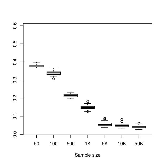
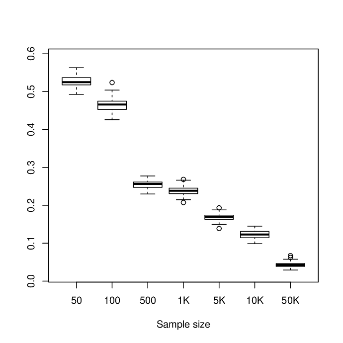
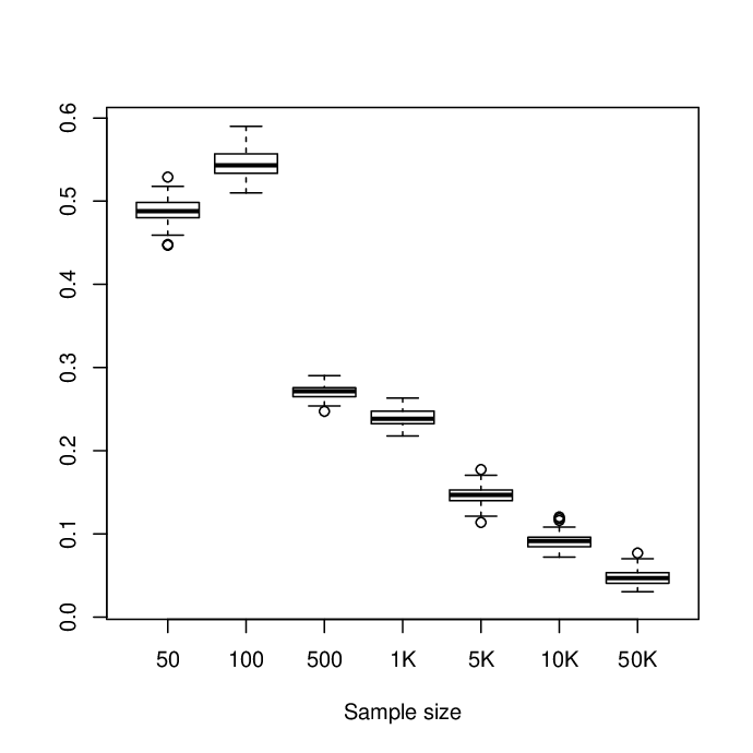
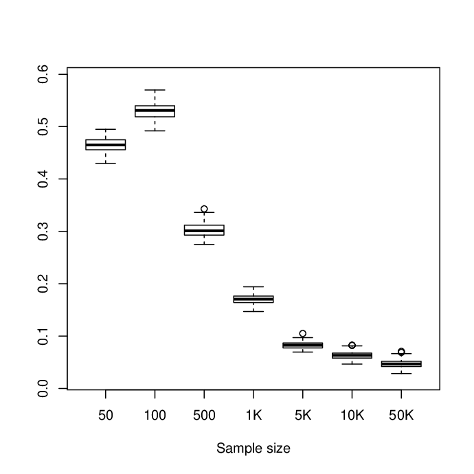
To assess convergence of the estimation error to the right weak limit, consider and to be respectively the empirical distributions of and for based on and independent replications. Here, and will be chosen to be large. More explicitly, a sample of independent random variables is drawn from for each to form a sample of size from the distribution of the estimation error. Note that this sample is multidimensional of dimension hence our need to consider the marginal components of its distribution. Similarly, we draw a sample of size from the distribution of weak limit using the algorithm described in Section 5.1. Define now
We will use this random variable to assess the established convergence. This is based on the fact that it is expected to become small for large . Since the “target ” distributions are , we choose . Also, we store those obtained empirical distributions and re-use them while sampling many times from the estimation error. This enables us to obtain independent realizations from while are fixed. To visualize the statistical summary of , the obtained outcomes are represented in the form of boxplots. Those were based on 100 replications of . Here, , and . In the simulations, we have taken the following true convex pmf’s which are all supported on :
- •
The triangular pmf , that is
- •
- •
The pmf, , of a truncated Geometric pmf with success probability equal to , that is
Note that if a geometric pmf is always convex on , this is not the case anymore after truncation. Indeed, convexity of the latter version holds true if and only if the waiting probability is . A simple proof of this fact can be found in Section 6.
Lemma 5.1.
Let be a positive integer and . The truncated Geometric distribution, defined by
and for all integers , is convex if and anly if .
To compute the uniform distance between and , we computed the maximal value of the absolute difference on a discretized grid with a regular step equal to . The boxplots shown in Figures 3 - 8 give support to the asymptotic theory of the estimation error of the MLE in case the true pmf is one of the selected convex pmf’s . Interestingly, weak convergence seems not to happen at the same speed. For the triangular pmf , the boxplots appear to stabilize for whereas the obtained boxplots for the other distributions seem to indicate that convergence has not been yet attained. According to our numerical findings in Section 5.2, large sample sizes could be required for the estimator to be able to capture these knots. Thus, the slow convergence to the true limit for could be partially explained by the fact that the pmf’s have all interior knots, as opposed the relatively fast convergence in the case of the triangular pmf which has none. We would like to note that all points in are interior knots of the truncated geometric pmf since it is strictly convex of its support. Hence, it is the pmf with the largest number of interior knots and also the one for which the convergence seems to be the slowest. Also, the limit reduces in this particular case to . Indeed, the empirical pmf is convex for large sample sizes (see Proposition 3.3) so that , and hence has the same limit distribution as Another way of viewing this is to note that the required convexity of the minimizer between the knots becomes a superfluous constraint since it is always satisfied by the straight line connecting at two given knots. This is true only in this case because all knots are consecutive.
We would like to finish this section by adding that it is of course impossible to have a precise statement about the speed of convergence in case the true convex pmf is known to be finitely supported. However, our numerical findings indicate that in applications such as construction of asymptotic confidence bands, one has to keep in mind that moderate sample sizes may not be enough to obtain good coverage. Finally, note that in our assessment we have assumed that the distribution of is continuous. We believe this is true but we do not intend to prove it here as it is beyond the scope of this work.


6 Proofs
Before showing Proposition 3.2, we note that the following inequalities hold true for any sequence . For , we have that
| (6.21) |
and
| (6.22) |
Proof of Proposition 3.2. The claim is an immediate consequence of Theorem 4 of Durot et al. (2013). Indeed, by the inequality in (6.22) we have that
almost surely by the Glivenko-Cantelli Theorem. Now, by the inequality in (6.21) and Theorem 4 of Durot et al. (2013) we can write
which completes the proof.
Proof of Theorem 3.4. Theorem 6 of Durot et al. (2013) implies (3.7) when . Let denote again the support of . By Theorem 1 of Durot et al. (2013), is a proper pmf. Combining this with Proposition 3.5, it follows that for . Hence, for all we have that
Also, the definition of and and Proposition 3.5 imply that for all
and the result follows.
Proof of Proposition 3.5. First, note that the maximal point of the support of the empirical pmf is , and that with probability one, provided that is sufficiently large. Now, by Theorem 1 of Durot et al. (2013) we know that admits a finite support whose maximal point . Therefore, with probability one we have for large enough. We show now by contradiction that with probability one there exists such that if then . Suppose that . By Proposition 1 of Durot et al. (2013) we know that with probability one there exists such that for , has to be linear on the set . But is a knot of which implies by Proposition 3.3 above that with probability one there exits such that for , is also a knot of . This yields a contradiction.
Proof of Theorem 4.1. First note that is a closed convex cone of , so there exists a unique minimizer of over .
Now suppose that is the minimizer of over . Let . Then, for the function is clearly in . Hence,
Recall that is the function defined as
For notational convenience, we set . Then, we can rewrite the last inequality as
where the last inequality follows from the fact that
together with the fact that for , and for . Thus,
for all . Note that at , equality of and is guaranteed by the chosen convention. Proof of equality in case is a knot of in uses the fact that the perturbation function satisfies that is in for small enough yielding
We also have equality of and at the points in since at these points there is no constraint.
Therefore, if is the minimizer of , we have shown that the process defined on as in (4.10) satisfies the inequality and equality in (4.11). Conversely, suppose that such that the process in (4.10) satisfies (4.11). Let . We will show now that . We have
where . Now, similar as above, for all we have
| (6.23) | |||||
with equality if is a knot of or . To conclude, we will use the fact that an arbitrary element can be written as
| (6.24) |
for all , with the knots of in for , and where are real numbers, and for and . This comes from the fact that any finite convex sequence for some , admits the (spline) representation
| (6.25) |
where is a real number, and are the interior knots of . Using the spline representation in (6.24) together with (6.23), where we recall that we have an equality for , it follows that
where in the last inequality we used the fact that for all . Now, the boundary conditions and in (4.11) imply that
since and is a standard Brownian bridge. We arrive at
and similarly, since we have an equality in (6.23) if is a knot of ,
It follows that and that is the minimizer of .
It follows from the characterization of in (3.6) that
By standard results on weak convergence of empirical processes we have that
Now, Theorem 3.4 implies that there exists a subsequence which weakly converges to some on . In what follows, we will use the Skorokhod representation to assume that convergences of and to their respective limits happen almost surely. The goal now is to show that and , defined in Theorem 4.1 above, are equal with probability one. Let us define
for with . Note that we have that
| (6.26) |
Indeed, by Fubini’s theorem we have that
This in turn implies that
and the claim follows by passing . Hence, with probability one we have that
Equality of and at points in in the last assertion follows from the chosen convention at , Proposition 3.3, the equalities for with probability one and large enough and the identity in (6.26). Equality of and at the knots of in follows from the fact that is a knot of in if and only if it is a knot of using linearity of between two successive knots. Thus, if is a knot of , then as soon as is large enough is also a knot of
This in turn implies that implying after passing to the limit that almost surely. Furthermore, is clearly in .
Therefore, it follows from Theorem 4.1 that must be equal to the minimizer of defined in (4.9). Thus, there exists a version of such that
for . Put . Then, for , we have that . Thus, since and . We conclude that since . Since we also have , it follows that on . Now, from an arbitrary subsequence we can extract a further subsequence converging to . Since the limit is the same for any such subsequence, we conclude that converges weakly to on with probability one. This in turn implies that the following converges
and
occur jointly, and the proof is complete.
Proof of Theorem 4.3. Existence and uniqueness of the minimizer both follow from the projection theorem on closed convex cones in . With similar arguments as for the proof of Theorem 4.1, it can be shown that an arbitrary element is the minimizer if and only if the process defined on by
satisfies
for all , with an equality if or is a knot of in for some with . Consider the restriction of to . A point is a knot of if, and only if, it is a knot of . Therefore, it immediately follows from the characterization of given in Theorem 4.1 that the minimizer of over is equal to if, and only if, . Since we already have , this is equivalent to
that is (4.14).
To prove the last assertion, note that from Theorem 4.2, it follows that converges in distribution to as . Thus, it converges in distribution to the minimizer of over if, and only if, (4.14) holds true with probability one. On the other hand, fromTheorem 4.2, one also has
| (6.27) |
as . Therefore, one can have (4.14) with probability one if, and only if,
converges in probability to zero as . This is equivalent to (4.15), so the proof of the theorem is complete.
Proof of Theorem 4.4. Existence and uniqueness of the minimizer both follow from the projection theorem on closed convex cones in . With similar arguments as for the proof of Theorem 4.1, it can be shown that an arbitrary element is the minimizer if and only if the process defined on by
satisfies
for all , with an equality if or is a knot of in for some with , where and
for all . The connection between and is as follows. For all one has
Similarly,
for all , so that
| (6.28) |
using that .
Consider . A point is a knot of if, and only if, it is a knot of . Therefore, it immediately follows from the characterization of given in Theorem 4.1, together with (6.28), that the minimizer of over is equal to if, and only if, . Since we already have , this is equivalent to
that is (4.16).
To prove the last assertion, note that from Theorem 4.2, it follows that converges in distribution to as . Thus, it converges in distribution to the minimizer of over if, and only if, (4.16) holds true with probability one. According to (6.27), this happens if, and only if,
converges in probability to zero as . This is equivalent to (4.17), so the proof of the theorem is complete.
Characterizing convexity for a truncated geometric pmf. A truncated pmf on with success probability is given by
Hence, is convex on if and only if
or equivalently
that is .
Proof of Lemma 5.1. We have for all by convexity of the function . We also have for all integers since for those , . Now, , and
which is if, and only if, . We conclude that for all if, and only if, .
Acknowledgments
The authors are very grateful to Sylvie Huet for many helpful comments, stimulating discussions on the subject, and also for a careful reading of the paper.
References
- Balabdaoui et al. (2013) Balabdaoui, F., Jankowski, H., Rufibach, K. and Pavlides, M. (2013). Asymoptic distribution of the discrete log-concave mle and some applications. JRSS-B. 75 769–790.
- Balabdaoui et al. (2009) Balabdaoui, F., Rufibach, K. and Wellner, J. A. (2009). Limit distribution theory for maximum likelihood estimation of a log-concave density. Annals of statistics 37 1299.
- Barlow et al. (1972) Barlow, R. E., Bartholomew, D. J., Bremner, J. and Brunk, H. (1972). Statistical inference under order restrictions: The theory and application of isotonic regression. Wiley New York.
- Dümbgen and Rufibach (2009) Dümbgen, L. and Rufibach, K. (2009). Maximum likelihood estimation of a log-concave density and its distribution function: Basic properties and uniform consistency. Bernoulli 15 40–68.
- Dümbgen and Rufibach (2010) Dümbgen, L. and Rufibach, K. (2010). logcondens: Computations related to univariate log-concave density estimation. Journal of Statistical Software, to appear .
- Durot et al. (2013)
Durot, C., Huet, S., Koladjo, F. and Robin,
S. (2013).
Least-squares estimation of a convex discrete distribution.
Comput. Statist. Data Anal. 67 282–298.
URL http://dx.doi.org/10.1016/j.csda.2013.04.019 - Durot et al. (2014) Durot, C., Huet, S., Koladjo, F. and Robin, S. (2014). Nonparametric species richness estimation under convexity constraint. Working paper .
- Durot et al. (2012) Durot, C., Kulikov, V. N., Lopuhaä, H. P. et al. (2012). The limit distribution of the -error of grenander-type estimators. The Annals of Statistics 40 1578–1608.
- Dykstra (1983) Dykstra, R. L. (1983). An algorithm for restricted least squares regression. Journal of the American Statistical Association 78 837–842.
- Grenander (1956) Grenander, U. (1956). On the theory of mortality measurement. Scandinavian Actuarial Journal 1956 125–153.
- Groeneboom et al. (2008a) Groeneboom, P., Jongbloeb, G. and Wellner, J. A. (2008a). The support reduction algorithm for computing nonparametric function estimates in mixture models. Scandinavian Journal of Statistics. 35 385–399.
- Groeneboom et al. (2001a) Groeneboom, P., Jongbloed, G. and Wellner, J. A. (2001a). A canonical process for estimation of convex functions: the “invelope” of integrated Brownian motion . Ann. Statist. 29 1620–1652.
- Groeneboom et al. (2001b) Groeneboom, P., Jongbloed, G. and Wellner, J. A. (2001b). Estimation of a convex function: characterizations and asymptotic theory. Ann. Statist. 29 1653–1698.
- Groeneboom et al. (2008b) Groeneboom, P., Jongbloed, G. and Wellner, J. A. (2008b). The support reduction algorithm for computing non-parametric function estimates in mixture models. Scandinavian Journal of Statistics 35 385–399.
- Holm and Frisén (1985) Holm, S. and Frisén, M. (1985). Nonparametric regression with simple curve characteristics. Research report 4, Dept. Statistics, Univ. Göteborg.
- Jankowski and Wellner (2009) Jankowski, H. K. and Wellner, J. A. (2009). Estimation of a discrete monotone distribution. Electron. J. Stat. 3 1567–1605.
- Kulikov et al. (2005) Kulikov, V. N., Lopuhaä, H. P. et al. (2005). Asymptotic normality of the lk-error of the grenander estimator. The Annals of Statistics 33 2228–2255.
- Mammen (1991) Mammen, E. (1991). Nonparametric regression under qualitative smoothness assumptions. The Annals of Statistics 19 741–759.
- Ng and Maechler (2007) Ng, P. and Maechler, M. (2007). A fast and efficient implementation of qualitatively constrained quantile smoothing splines. Statistical Modelling 7 315–328.
- NG and Maechler (2007) NG, P. and Maechler, M. (2007). A fast and efficient implementation of qualitatively constrained quantile smoothing splines. Statistical Modelling 7 315–328.
- Prakasa Rao (1969) Prakasa Rao, B. (1969). Estimation of a unimodal density. Sankhyā: The Indian Journal of Statistics, Series A 23–36.