CONVERGENCE AND ERROR PROPAGATION RESULTS ON A LINEAR ITERATIVE UNFOLDING METHOD

ANDRÁS LÁSZLÓ ^†^†thanks: Wigner Research Centre for Physics, Konkoly-Thege M.u. 29-33, Budapest, H-1121, Hungary. (e-mail: ). Email: laszlo.andras@wigner.mta.hu

Abstract

Unfolding problems often arise in the context of statistical data analysis. Such problematics occur when the probability distribution of a physical quantity is to be measured, but it is randomized (smeared) by some well understood process, such as a non-ideal detector response or a well described physical phenomenon. In such case it is said that the original probability distribution of interest is folded by a known response function. The reconstruction of the original probability distribution from the measured one is called unfolding. That technically involves evaluation of the non-bounded inverse of an integral operator over the space of $L^{1}$ functions, which is known to be an ill-posed problem. For the pertinent regularized operator inversion, we propose a linear iterative formula and provide proof of convergence in a probability theory context. Furthermore, we provide formulae for error estimates at finite iteration stopping order which are of utmost importance in practical applications: the approximation error, the propagated statistical error, and the propagated systematic error can be quantified. The arguments are based on the Riesz-Thorin theorem mapping the original $L^{1}$ problem to $L^{2}$ space, and subsequent application of ordinary $L^{2}$ spectral theory of operators. A library implementation in C of the algorithm along with corresponding error propagation is also provided. A numerical example also illustrates the method in operation.

keywords

unfolding; convergence; error propagation; probability theory; statistics; functional analysis; Riesz-Thorin theorem

AMS

46E30; 46E27; 62H99

\slugger

sinumxxxxxxxx–x

1 Introduction

In analysis of experimental data one commonly faces the problem that the probability density function (pdf) of a given physical quantity of interest is to be measured, but some random physical process, such as the intrinsic behavior of the measurement apparatus smears it. The reconstruction of the pertinent unknown pdf of interest based on the observed smeared pdf and on the known response function of the measurement procedure is called unfolding.

More specifically, one of the most common unfolding scenarios turning up in experimental data analysis is the following. Let $x\mapsto f(x)$ be the unknown pdf which we intend to reconstruct, $(y,x)\mapsto\rho(y|x)$ be the known response function of the smearing effect, and we assume that $y\mapsto g(y)=\int\rho(y|x)\,f(x)\,\mathrm{d}x$ is the measured pdf after the smearing effect, called folding. In practice, actually often only a statistical estimator of $g$ can be measured. Or, putting it differently, $g$ often contains an additional error term $y\mapsto e(y)$ originating from statistical counting and unaccounted systematic measurement distortions, in which case one has $y\mapsto g(y)=\int\rho(y|x)\,f(x)\,\mathrm{d}x\,+\,e(y)$ as the measured pdf estimator. The task of unfolding is to provide some close estimate for $x\mapsto f(x)$ , given $y\mapsto g(y)$ and $(y,x)\mapsto\rho(y|x)$ along with some estimate on $y\mapsto e(y)$ , i.e. to solve the above linear integral equation. It is quite well known in the literature that such a problem is numerically ill-posed. The primary reason for this is Banach’s closed graph theorem: due to the pertinent theorem a generic folding operator maps certain distant pdfs to close ones whose differences after the folding are shadowed by the contribution of the measurement error term $e$ . That quite well understood phenomenon is summarized e.g. in [1, 2, 3, 4, 5, 6, 7, 8].

The problematics of unfolding can also be formulated using a language possibly more familiar to statisticians [9, 10]. Let $x_{1},\dots,x_{n}$ be statistical instances of a probability variable $x$ , i.e. independent identically distributed random variables, each having the same but unknown pdf $f$ . In the experimental setting, merely the random variables $y_{i}=x_{i}+\varepsilon_{x_{i},i}$ ( $i=1,\dots,n$ ) are observed, i.e. the original $x_{i}$ ( $i=1,\dots,n$ ) random variables corrupted by an $x$ -dependent, but otherwise independent identically distributed error variable $\varepsilon_{x}$ , having a known $x$ -dependent pdf $\varepsilon_{x}\mapsto\rho(\varepsilon_{x}+x|x)$ for each fixed value of $x$ as a condition. Given all these, the task of unfolding is to provide an estimator for the pdf $f$ of the undistorted probability variable $x$ . In some real experimental situation, it also happens that the individual observed samples $y_{i}=x_{i}+\varepsilon_{x_{i},i}$ ( $i=1,\dots,n$ ) are not published, only their pdf estimator $g$ is made available, for instance because there is some correction procedure on the pdf level, e.g. for inefficiencies. Also, our model $(y,x)\mapsto\rho(y|x)$ for the response function might be systematically inaccurate, for which inaccuracy only an upper bound might be known. Therefore, often not the sample based observational model, but rather the previously discussed pdf estimator based observational model is more practical to handle. But whichever way the problem is formulated — based on individual samples or on pdfs — the task remains to be ill-posed.

In order to overcome the ill-posedness of the unfolding problem, all the methods use restrictions on the unknown pdf, and in some special cases properties of the response function can also be used to improve the situation. For instance, in the field of image or signal processing, the shape of the response function is translationally invariant in an exact manner, i.e. for all $x,y,z$ one has $\rho(y|x+z)=\rho(y-z|x)$ , and thus the unfolding reduces to the problematics of deconvolution. In the language of statistical samples, this would correspond to the observational model when $y_{i}=x_{i}+\varepsilon_{i}$ ( $i=1,\dots,n$ ) are observed, with independent identically distributed random variables $\varepsilon_{i}$ of a known distribution, not depending on $x$ . Due to the applicational importance of the special case of deconvolution problems, that branch has a whole stream of literature [9, 10, 11, 12, 13, 14, 15, 16]. The statistical deconvolution methods heavily rely on the applicability of convolution theorem for the Fourier transformed pdfs, which is possible due to the translational invariance of the shape of the response function, i.e. relies on the fact that the probability variables $\varepsilon_{i}$ ( $i=1,\dots,n$ ) are independent identically distributed and are independent from $x$ . The ill-posedness of the problem, similarly to the case of any generic unfolding method, is regularized by finding and approximative solution. The optimal approximation is controlled by the application of the minimax principle: for a given estimate of the true deconvolved pdf, a loss (penalty) function is defined, and the minimum of the worst case expected loss is looked for as a function of the regularization parameters. It is worth to note that most of the advanced statistical deconvolution methods can work on unbinned samples, i.e. they do not need an a priori histograming of the observed data. In Section 6 an illustrative numerical unfolding toy model application is presented, which also tries to clarify that in an experimental context more general approaches than deconvolution are also needed in order to handle real measurement situations.

Also in the case of generic — i.e. non-deconvolution — unfolding problems a regularization method must be applied [1, 3, 4, 5, 6, 7, 8, 16, 17, 18, 19] and an approximate solution of the folding integral equation within a reduced set of allowed pdfs is searched for. The approximation is controlled by some regularization parameters whose particular value brings in a certain degree of arbitrariness to the unfolded pdf (approximation error), which is often difficult to quantify. There are basically three main widespread ways in the literature addressing the problem of regularization.

(i)

In certain data analysis problems a parametric ansatz for the unknown pdf $f$ is justified. In that case, one can construct the folded version of $f$ by the response function $\rho$ numerically, and that can be fitted to the observed folded pdf $g$ , for instance via a maximum likelihood method. Such method is used for instance in inclusive particle identification in experimental high energy particle physics (see for instance [20]). Due to the ill-posedness of the unfolding problem, one may run into a situation in particular cases when the fit is insensitive to some details of the parametrically given $f$ . In other words: the log-likelihood function ( $\chi^{2}$ ) may be flat in the direction of certain parameters of the ansatz for $f$ .
(ii)

Bin-by-bin fitting of the histogramed $f$ , such that when numerically folding it by $\rho$ the result gets close to the observed folded pdf $g$ , e.g. in a maximum likelihood sense. This is very similar to approach (i) with every bin amplitude of the histogramed $f$ being a fit parameter. This method is basically equivalent to the naive inversion of the discretized folding operator as a matrix. Due to the ill-posedness of the unfolding problem, this is not satisfactory in itself. The usual procedure is to add some artificial penalty function to the log-likelihood function ( $\chi^{2}$ ) in order to suppress the large local gradients. If that is performed, the method can deliver meaningful answers, but the introduced systematic bias by the additional penalty function is difficult to quantify. In addition, similarly to the method (i), the fit can be slightly insensitive to the details of $f$ due to the ill-posedness of the problem. The so called SVD methods [17] are implementations of this idea.
(iii)

There are also iterative methods which intend to approximate the true pdf $f$ , given the measured folded pdf $g$ and the response function $\rho$ . One of the most popular and most promising methods is the method of convergent weights, also called iterative Bayesian unfolding. It was first discovered and applied by Richardson [21] and Lucy [22] for image processing. Later it was re-discovered and applied to tomography problems by Shepp and Vardi [23], and by Kondor [24]. The first serious mathematical scrutiny of the method was done by Mülthei and Schorr [25, 26]. In the mid-90s d’Agostini re-discovered and popularized the algorithm in the high energy physics community [18]. Recently, Zech [19] studied possible optimal iteration stopping criteria for the algorithm. One of the main advantages of the method of convergent weights or Bayesian unfolding is, that it takes into account the non-negativity and the unitness of the integral of the true pdf $f$ in an exact manner. Furthermore, if the measured folded pdf $g$ was a histogram, i.e. its values fluctuate according to Poisson counting statistics, then the iterative approximants to $f$ have increasing likelihood [25], i.e. the algorithm is a realization of a maximum-likelihood approximation. Most unfortunately, despite of the research efforts [25], there are no results stating that the method is convergent, although numerical evidence suggests its convergent nature. Moreover, there are no exact error propagation formulae available.

In case of a consistent method the approximation error should converge to zero when the regularization parameters are relaxed. In case of an iterative method, an approximating sequence $\left(f_{N}\right)_{N\in\mathbb{N}_{0}}$ to the unknown $f$ is constructed and the regularization parameter is merely the iteration stopping order $N_{\mathrm{max}}$ , i.e. a threshold index in the approximating sequence. When an iterative unfolding method is consistent, the approximation error, i.e. the distance of $f_{N}$ to the true unknown $f$ must converge to zero with increasing number of iterations $N$ . Although the above consistency property is an obvious minimal requirement for any unfolding method, often this is not easy to show analytically.

In a previous paper [1] we proposed a linear iterative unfolding method, discussed its pros and cons in comparison to other techniques, provided detailed description from the practical point of view for experimentalists, along with providing a set of relevant application examples. In the present paper we provide formal mathematical proofs for the claims therein for the proposed unfolding method:

(i)

proof of consistency, i.e. that the approximation error converges to zero with increasing number of iterations,
(ii)

explicit formula for the approximation error at finite iteration order,
(iii)

explicit formula for the propagated statistical errors on the unfolded pdf at finite iteration order given the statistical errors of the measured folded pdf,
(iv)

explicit formula for the propagated systematic errors on the unfolded pdf at finite iteration order given the systematic errors of the measured folded pdf or of the response function.

Because of (ii)–(iv) the competing error terms become calculable, and therefore these can be used to define an optimal iteration stopping criterion. In addition, the pertinent error terms can be determined at this optimum. The quantification of these are of utmost importance when presenting unfolded experimental results, and is generally an unresolved task for other widely used unfolding methods. The key mathematical ingredient of the proofs are mapping our originally $L^{1}$ problem to the $L^{2}$ space using Riesz-Thorin theorem, and using spectral representation of the operators therein. The actual iteration formula is formally motivated by a preconditioned Neumann-Landweber-Richardson series, but these are not automatically convergent in case of $L^{1}$ problems: our specific preconditioning makes the iteration convergent in the $L^{1}$ setting, given some quite generic conditions. The proposed method also does not rely on an inherent discretization of the pdfs: it does work also in the continuum limit or with any type of density estimators.¹¹ 1 Some unfolding methods rely on an inherent discretization of pdfs in the problem, and use the assumed discretization as an implicit regularization. Our method does not use such trick.

The obtained results can be particularly interesting as the proposed method can be considered as the “linearized” version of the method of convergent weights or iterative Bayesian unfolding [18, 19, 21, 22, 23, 24, 25, 26]. By understanding the convergence conditions and error propagation for the proposed method, the studies of Mülthei and Schorr [25] could eventually be completed on the Bayesian iteration, which would be a significant improvement in the field.

The paper is organized as follows: in Section 2 the problem of unfolding is introduced in a mathematically rigorous way, and the basic properties of generic folding operators are discussed. In Section 3 our proposed unfolding method is introduced and proofs are provided for its above listed properties. In Section 4 we generalize a bit our results for the case of probability measures which are not described by pdfs. In Section 5 we restrict our results to the special case when the unfolding problem is discrete: this presentation may be better understood by statisticians or experimental physicists not specialized in functional analysis. In Section 6 a concrete numerical example is shown. Finally, in Section 7 we summarize.

2 Mathematical properties of folding operators and the unfolding

In the text we shall abbreviate by pdf the notion of probability density function, by cpdf the notion of conditional probability density function. We shall rely on the usual terminology in functional analysis and measure theory [27, 28]. As such, the notion of Lebesgue almost everywhere or Lebesgue almost every, shall be abbreviated by a.e.

Let $X$ and $Y$ be finite dimensional real vector spaces equipped with the Lebesgue measure — unique up to a global positive normalization factor. Let $L^{1}(X)$ and $L^{1}(Y)$ denote the Banach spaces of $X\rightarrow\mathbb{C}$ and $Y\rightarrow\mathbb{C}$ Lebesgue integrable function equivalence classes, respectively, where the equivalence of functions is defined by being a.e. equal. As usual in functional analysis texts, we shall call these function equivalence classes simply functions. We shall also use the notion of essential bound for such a function which is the smallest upper bound valid a.e.

Definition 1.

Let $\rho:\,Y\times X\rightarrow\mathbb{R}_{0}^{+},\,(y,x)\mapsto\rho(y|x)$ be a cpdf over the product space $Y\times X$ , i.e. a non-negative Lebesgue measurable function which satisfies $\forall x\in X:\,\int\rho(y|x)\,\mathrm{d}y=1$ . Then, the linear operator

(1)

\displaystyle A_{\rho}\;:\;L^{1}(X)\rightarrow L^{1}(Y),\;(x\mapsto f(x))\,\mapsto\,\left(y\mapsto\int\rho(y|x)\,f(x)\,\mathrm{d}x\right)

is called the folding operator by $\rho$ , where the function $\rho$ is called the response function of the folding.

Remark 2.1.

The following basic properties of folding operators are direct consequences of the definition.

(i)

A possible usual generalization of the notion of folding operator is when inefficiencies are also allowed, i.e. the less restrictive condition $\forall x\in X:\,\int\rho(y|x)\,\mathrm{d}y\leq 1$ is required for the response function $\rho$ of the folding operator $A_{\rho}$ . The results throughout the paper are also valid for that case.
(ii)

By Fubini’s theorem, a folding is a well defined linear operator.
(iii)

It is also quite evident [2] that such operator is continuous in the $L^{1}$ operator norm (i.e. in probabilistic sense), moreover $\|A_{\rho}\|_{L^{1}(X)\rightarrow L^{1}(Y)}=1$ , while $\|A_{\rho}\|_{L^{1}(X)\rightarrow L^{1}(Y)}\leq 1$ whenever inefficiencies are allowed.

It is seen that such a folding operator $A_{\rho}$ is quite well behaved: it is linear and is continuous in the probabilistic sense, i.e. close pdfs are mapped to close pdfs in the $L^{1}$ sense [1].

A quite important class of folding operators are convolutions, in which case the shape of the response function is translationally invariant.

Definition 2.

A folding operator $A_{\rho}$ is called convolution whenever the response function $\rho$ is translationally invariant in the sense that $Y=X$ and $\forall x,y,z\in X\,:\,\rho(y|x+z)=\rho(y-z|x)$ .

Remark 2.2.

The following properties of convolution operators are well-known results [2, 29, 30].

(i)

In case a folding operator $A_{\rho}$ is a convolution, the response function $\rho$ may be expressed by the single pdf $\eta:=\rho(\cdot|0)$ in the form $\forall x,y\in X:\,\rho(y|x)=\eta(y-x)$ . The alternative notation $\eta\star f:=A_{\rho}f$ is often used in such case ( $f\in L^{1}(X)$ ). Note that convolution is commutative, i.e. one has $\eta\star f=f\star\eta$ for all $\eta,f\in L^{1}(X)$ .
(ii)

A convolution operator is not onto, and its image is not closed.
(iii)

The image of a convolution operator is dense if and only if the Fourier transform of the convolver function is nowhere zero (Wiener’s approximation theorem).
(iv)

A convolution operator is one-to-one if and only if the Fourier transform of the convolver function is a.e. nonzero.
(v)

Consequently, the inverse of a convolution operator, whenever exists, cannot be continuous. This is because a convolution is everywhere defined on the closed set $L^{1}(X)$ , it is continuous, and therefore it has closed graph by Banach’s closed graph theorem; but since the inverse operator’s domain is not closed, again by Banach’s closed graph theorem, it cannot be continuous.

Since the convolution operators form a quite large example class of folding operators, we can state that a generic folding operator’s inverse, whenever exists, is not continuous. This finding is often referred to as: the inversion of a generic folding operator is ill-posed. The argument goes as follows: we have an unknown pdf $f$ , a known response function $\rho$ , and a measured pdf $g=A_{\rho}f+e$ where $e$ represents a small measurement error term. Then, when one would set $A_{\rho}^{-1}g=f+A_{\rho}^{-1}e$ , the error term $e$ contains modes not in the domain of $A_{\rho}^{-1}$ in which case $A_{\rho}^{-1}e$ is not meaningful, or when approximated numerically, this term shall diverge. Note that even if all modes of $e$ were in the domain of $A_{\rho}^{-1}$ , the smallness of $A_{\rho}^{-1}e$ is not guaranteed even though $e$ is small. The ill-posedness of a generic unfolding problem may also be stated as: if $f_{1}$ and $f_{2}$ are distant pdfs, then $g_{1}:=A_{\rho}f_{1}+e_{1}$ and $g_{2}:=A_{\rho}f_{2}+e_{2}$ may be close pdfs, i.e. we lose discrimination power on pdfs after a folding [1]. The presented argument also warns us against relying solely on the so called closure test when verifying an unfolding algorithm: whenever some unfolding method gives some estimate $\hat{f}$ for the unknown pdf $f$ , it is usually argued that $A_{\rho}\hat{f}\approx A_{\rho}f$ confirms the validity of the estimate $\hat{f}$ . Clearly, in the light of our observations this is not enough, as $\hat{f}$ may be still far from $f$ in the probabilistic distance.

Due to the ill-posedness of the unfolding problem, any unfolding method needs to use some kind of regularization: some assumption on the original (unknown) pdf, and a way to search for an approximative solution depending on some regularization parameters. Furthermore, the convergence to the original pdf when relaxing these parameters can usually be only achieved in some weak sense, not in the probabilistic norm of $L^{1}(X)$ . The most commonly applied unfolding strategies are summarized in [1, 3, 4, 5, 6, 7, 8, 16, 17, 18, 19].

3 A linear iterative unfolding method

Since the folding equation Eq.(1) is linear, it is quite natural to try applying some iterative inversion methods known in functional analysis, when approximating the true solution $f$ . One such self-suggesting method is Neumann series [27, 28] which guarantees that whenever for a continuous linear operator $A$ over a Banach space one has $\|I-A\|<1$ ( $I$ being the identity operator), then $A^{-1}=\sum_{n=0}^{\infty}(I-A)^{n}$ where the convergence holds in the operator norm. That convergence requirement, however, cannot be satisfied in case of a probability theory folding operator because for such an operator one has $\|I-A_{\rho}\|_{L^{1}\rightarrow L^{1}}=2$ as shown in [2]. The Richardson iteration, based on similar requirements, does not work for the same reason. An other evident choice would be the Landweber iteration [31] known in the theory of Fredholm integral equations [27, 28]. This assumes, in first place, that the unknown function $f$ and the result of the folding $g$ resides in the space of square integrable functions $L^{2}(X)$ , furthermore that the response function $\rho$ satisfies the regularity condition $\int\int\big|\rho(y|x)\big|^{2}\,\mathrm{d}y\,\mathrm{d}x<\infty$ . The latter regularity condition, unfortunately, is violated in case of a generic cpdf, on the contrary to the common belief in the literature.²² 2 It is evidently seen that this regularity condition does not hold for any convolution. It is also seen at the price of some calculation that this situation cannot be repaired by a compactification mapping, i.e. if we map the support set of our pdfs and response function into a compact region of $Y$ and $X$ .

Despite of the fact that neither the Neumann series, nor the Richardson iteration, nor the Landweber iteration can be directly applied to an unfolding problem, they provide a possible starting point. Motivated by these algorithms we proposed a linear iterative unfolding method for a probability theory context, i.e. for the $L^{1}$ space [1]. The section is continued by recalling notions necessary for studying the pertinent algorithm.

In the followings we shall denote by $L^{p}(X)$ the Banach space of $X\rightarrow\mathbb{C}$ functions [27, 28] which are Lebesgue integrable of the $p$ -th power ( $1\leq p\leq\infty$ ). The special case $L^{\infty}(X)$ for $p=\infty$ is defined as the Banach space of the $X\rightarrow\mathbb{C}$ essentially bounded functions with their norm being the essential bound.

Remark 3.1.

The argumentation in the followings relies on some known results.

(i)

The Riesz-Thorin theorem [32] states that if $1\leq q\leq r\leq\infty$ and $F\subset L^{q}(X)\cap L^{r}(X)$ is a dense linear subspace in both $L^{q}(X)$ and $L^{r}(X)$ , furthermore a linear operator $T:F\rightarrow L^{q}(X)\cap L^{r}(X)$ is bounded both in the $L^{q}(X)$ and $L^{r}(X)$ norm, then for all $q\leq p\leq r$ values $F\subset L^{p}(X)$ , it is dense in $L^{p}(X)$ , $T[F]\subset L^{p}(X)$ and $T$ is bounded in the $L^{p}(X)$ norm. Thus, $T$ is uniquely extendable as an $L^{p}(X)\rightarrow L^{p}(X)$ bounded linear operator. In addition we have that

(2)

\displaystyle\left\|T\right\|_{L^{p}\rightarrow L^{p}}\leq\max\left(\left\|T\right\|_{L^{q}\rightarrow L^{q}},\left\|T\right\|_{L^{r}\rightarrow L^{r}}\right)

holds for the operator norms.

(ii)

An important consequence of the Riesz-Thorin theorem is that a convolution operator $\eta\star(\cdot)$ by a function $\eta\in L^{1}(X)$ is well defined and continuous in $L^{p}(X)$ for all $1\leq p\leq\infty$ and its operator norm is bounded by $\|\eta\|_{L^{1}}$ . This obviously holds for the $p=1$ and $p=\infty$ case due to Hölder’s inequality, and then it is implied for all $1<p<\infty$ as well by the pertinent theorem. As a consequence, using the commutativity of convolution, it also follows that if $\varphi\in L^{p}(X)$ and $\eta\in L^{1}(X)$ then $\varphi\star\eta\in L^{p}(X)$ , i.e. pdfs may be mapped into $L^{p}(X)$ via convolution by pdfs integrable on the $p$ -th power.
(iii)

We shall use in the followings the spectral representation [28] of normal operators over complex separable Hilbert spaces. Let $T$ be a normal operator over the pertinent space, i.e. a densely defined linear operator with closed graph, satisfying $T^{*}T=TT^{*}$ , $(\cdot)^{*}$ being the adjoint. Then there exists a unique projection valued measure $P$ over the Borel sets of the spectrum set of $T$ , $\mathrm{Sp}(T)$ , such that

(3) $\displaystyle T=\int_{\lambda\in\mathrm{Sp}(T)}\lambda\,\mathrm{d}P(\lambda)$

holds, where the integral is defined in the weak sense. That is, for all elements $f,g$ in the Hilbert space one has a complex valued Borel measure $\left<f,P(\cdot)g\right>$ such that

(4) $\displaystyle\left<f,Tg\right>=\int_{\lambda\in\mathrm{Sp}(T)}\lambda\;\mathrm{d}\left<f,P(\lambda)g\right>.$

In addition, one has that if $M$ is a polynomial, then $M(T)$ is also normal operator, furthermore

(5) $\displaystyle M(T)=\int_{\lambda\in\mathrm{Sp}(T)}M(\lambda)\,\mathrm{d}P(\lambda)$

is satisfied in the same sense.

Throughout the argumentation we will need the notion of transpose folding which is introduced below.

Definition 3.

If $A_{\rho}$ is a folding operator such that the response function $\rho(\cdot|x)$ is square-integrable for all $x\in X$ , then for all $k\in L^{2}(Y)$ the expression

(6)

\displaystyle A_{\rho}^{T}k:=\left(x\mapsto\int k(y)\,\rho(y|x)\,\mathrm{d}y\right)

is meaningful and defines a linear map from $L^{2}(Y)$ to the Lebesgue measurable functions $X\rightarrow\mathbb{C}$ . We call the linear operator $A_{\rho}^{T}$ the transpose folding.

3.1 The iterative approximation

Equipped with the listed notions, we can introduce the following approximating sequence for solution of the unfolding problem. Let $g=A_{\rho}f$ be our unfolding problem where $f$ is to be determined, with $g$ and $\rho$ being known. We try to approximate the solution in the form:

(7)	$\displaystyle K_{\rho}$	$\displaystyle:=$	$\displaystyle\sup_{x\in X}\int\int\rho(y\|z)\,\rho(y\|x)\,\mathrm{d}y\,\mathrm{d}z,$
(8)	$\displaystyle f_{0}$	$\displaystyle:=$	$\displaystyle K_{\rho}^{-1}A_{\rho}^{T}g,$
(9)	$\displaystyle f_{N+1}$	$\displaystyle:=$	$\displaystyle f_{N}+\left(f_{0}-K_{\rho}^{-1}A_{\rho}^{T}A_{\rho}f_{N}\right)$
(10)			$\displaystyle(N\in\mathbb{N}_{0}).$

This is, formally, the iterative expression for Neumann series after preconditioning by $K_{\rho}^{-1}A_{\rho}^{T}$ , i.e. for the composite operator $K_{\rho}^{-1}A_{\rho}^{T}A_{\rho}$ .

3.2 Convergence conditions

The following theorem shows that under quite generic conditions the approximating sequence $\left(f_{N}\right)_{N\in\mathbb{N}_{0}}$ in terms of Eq.(10) is well-defined and converges to $f$ whenever $A_{\rho}$ is one-to-one, and it converges to the closest possible function to $f$ whenever $A_{\rho}$ is not one-to-one.

Theorem 4.

(Convergence) Let $A_{\rho}$ be a folding operator and assume that its response function $\rho$ has the property that for all $x\in X$ the function $\rho(\cdot|x)$ is square-integrable, furthermore $K_{\rho}<\infty$ . Assume that the unknown pdf $f$ in the unfolding problem $g=A_{\rho}f$ is square-integrable. Then:

(i)

For any compact set $U\subset X$ :

(11)

\displaystyle\lim_{N\rightarrow\infty}\frac{1}{\mathrm{Volume}(U)}\int_{x\in U}\left(f-\mathcal{P}_{\mathrm{Ker}(A_{\rho})}f-f_{N}\right)(x)\,\mathrm{d}x=0,

where $\mathcal{P}_{\mathrm{Ker}(A_{\rho})}$ is the $L^{2}$ orthogonal projection onto the kernel set of $A_{\rho}$ .

(ii)

We have that

(12) $\displaystyle\lim_{N\rightarrow\infty}\left\|f-\mathcal{P}_{\mathrm{Ker}(A_{\rho})}f-f_{N}\right\|_{L^{2}}=0$

and the convergence is monotone.

Proof.

It is seen that whenever the regularity condition $\forall x\in X:\,\rho(\cdot|x)\in L^{2}(Y)$ holds, the function

(13)

\displaystyle\alpha\,:\;X\times X\rightarrow\mathbb{R}^{+}_{0},\;(z,x)\mapsto\alpha(z,x):=\int\rho(y|z)\rho(y|x)\,\mathrm{d}y

is well defined. By construction, it is symmetric, i.e. $\forall z,x\in X:\,\alpha(z,x)=\alpha(x,z)$ . Furthermore, because of $K_{\rho}<\infty$ and symmetricity,

(14)

\displaystyle\sup_{x\in X}\int_{z\in X}\alpha(z,x)\,\mathrm{d}z=\sup_{z\in X}\int_{x\in X}\alpha(z,x)\,\mathrm{d}x=K_{\rho}<\infty

holds. With this, we see that the operator $A_{\rho}^{T}A_{\rho}$ is well defined as $L^{1}(X)\rightarrow L^{1}(X)$ and is bounded, its $L^{1}\rightarrow L^{1}$ operator norm being $K_{\rho}$ . This is because for any $f\in L^{1}(X)$

(15)		$\displaystyle\left\\|A_{\rho}^{T}A_{\rho}f\right\\|_{L^{1}}=\int\left\|\int\alpha(z,x)f(x)\,\mathrm{d}x\right\|\,\mathrm{d}z$
(16)		$\displaystyle\qquad\leq\int\int\alpha(z,x)\left\|f(x)\right\|\,\mathrm{d}x\,\mathrm{d}z=\int\left(\int\alpha(z,x)\,\mathrm{d}z\right)\left\|f(x)\right\|\,\mathrm{d}x$
(17)		$\displaystyle\qquad\leq\sup_{x\in X}\left(\int_{z\in X}\alpha(z,x)\,\mathrm{d}z\right)\,\int_{x\in X}\left\|f(x)\right\|\,\mathrm{d}x=K_{\rho}\left\\|f\right\\|_{L^{1}}$

due to of monotonicity of integration, Fubini’s theorem and Hölder’s inequality. It is also seen that the operator $A_{\rho}^{T}A_{\rho}$ is well defined as $L^{\infty}(X)\rightarrow L^{\infty}(X)$ and is bounded, its $L^{\infty}\rightarrow L^{\infty}$ operator norm being $K_{\rho}$ . That is because for any $f\in L^{\infty}(X)$

(18)		$\displaystyle\left\\|A_{\rho}^{T}A_{\rho}f\right\\|_{L^{\infty}}=\sup_{z\in X}\left\|\int\alpha(z,x)f(x)\,\mathrm{d}x\right\|$
(19)		$\displaystyle\qquad\leq\sup_{z\in X}\int\alpha(z,x)\left\|f(x)\right\|\,\mathrm{d}x\leq\sup_{z\in X}\left(\int\alpha(z,x)\,\mathrm{d}x\sup_{x\in X}\left\|f(x)\right\|\right)$
(20)		$\displaystyle\qquad=\sup_{z\in X}\left(\int_{x\in X}\alpha(z,x)\,\mathrm{d}x\right)\,\sup_{x\in X}\left\|f(x)\right\|=K_{\rho}\left\\|f\right\\|_{L^{\infty}}$

due to monotonicity of integration and Hölder’s inequality.

Now, using Riesz-Thorin theorem we have that the operator $A_{\rho}^{T}A_{\rho}$ is well-defined as $L^{2}(X)\rightarrow L^{2}(X)$ and is bounded, its $L^{2}\rightarrow L^{2}$ operator norm being bound by $K_{\rho}$ . It is also easily seen that for any $f\in L^{2}(X)$ one has $\left<f,A_{\rho}^{T}A_{\rho}f\right>=\left<A_{\rho}f,A_{\rho}f\right>\geq 0$ , therefore it is a self adjoint and positive operator in $L^{2}(X)$ . Thus, its spectrum lies within the interval $[0,K_{\rho}]$ . For brevity, we introduce the notation $A:=K_{\rho}^{-1}A_{\rho}^{T}A_{\rho}$ for the re-normalized composite folding operator.

Let us observe that the iterative formula Eq.(10) may also be written in the series expansion form $f_{N}=\sum_{n=0}^{N}(I-A)^{n}f_{0}$ where we have that $f_{0}=Af$ , $f$ being the unknown pdf. This form is particularly useful because then we see by induction that $\sum_{n=0}^{N}(I-A)^{n}A=I-(I-A)^{N+1}$ , i.e. we have the explicit formula $f-f_{N}=(I-A)^{N+1}f$ for the residual term.

By the observed properties of $A$ it is quite evident that $\mathrm{Sp}(A)\subset[0,1]$ . Thus, there exists a unique projection valued measure $P$ on the Borel sets of $[0,1]$ such that

(21)

\displaystyle A=\int_{\lambda\in[0,1]}\lambda\,\mathrm{d}P(\lambda)

in the weak sense. This implies that for any $h\in L^{2}(X)$ we have

(22)	$\displaystyle\left<h,f-f_{N}\right>$	$\displaystyle=$	$\displaystyle\int_{\lambda\in[0,1]}(1-\lambda)^{N+1}\,\mathrm{d}\left<h,P(\lambda)f\right>$
(24)		$\displaystyle=$	$\displaystyle\int_{\lambda\in\{0\}}(1-\lambda)^{N+1}\,\mathrm{d}\left<h,P(\lambda)f\right>+$
(24)			$\displaystyle\int_{\lambda\in]0,1]}(1-\lambda)^{N+1}\,\mathrm{d}\left<h,P(\lambda)f\right>.$

Since $\int_{\lambda\in\{0\}}(1-\lambda)^{N+1}\,\mathrm{d}P(\lambda)=\mathcal{P}_{\mathrm{Ker}(A_{\rho})}$ for all $N\in\mathbb{N}_{0}$ , we arrive at the identity

(25)

\displaystyle\left<h,f-\mathcal{P}_{\mathrm{Ker}(A_{\rho})}f-f_{N}\right>=\int_{\lambda\in]0,1]}(1-\lambda)^{N+1}\,\mathrm{d}\left<h,P(\lambda)f\right>,

and by the monotonicity of integration

(26)

\displaystyle\left|\left<h,f-\mathcal{P}_{\mathrm{Ker}(A_{\rho})}f-f_{N}\right>\right|\leq\int_{\lambda\in]0,1]}\left|1-\lambda\right|^{N+1}\,\mathrm{d}\left|\left<h,P(\lambda)f\right>\right|

also holds, where the symbol $|\cdot|$ when applied to complex valued measures denotes variation, which is analogous to absolute value of complex valued functions. The measure $\left<h,P(\cdot)f\right>$ on $[0,1]$ has finite variation and the function sequence $\lambda\mapsto(1-\lambda)^{N+1}$ ( $N\in\mathbb{N}_{0}$ ) is bounded independently of $N$ and converges pointwise to zero on $]0,1]$ , therefore by Lebesgue’s theorem of dominated convergence [27, 28] we have that the sequence of integrals converges to zero. Thus, the first part of the theorem is proved by setting $h:=\frac{1}{\mathrm{Volume}(U)}\,\chi_{{}_{U}}$ .

The second part of the theorem is proved by observing that

(27)		$\displaystyle\left\\|f-\mathcal{P}_{\mathrm{Ker}(A_{\rho})}f-f_{N}\right\\|_{L^{2}}^{2}$	$\displaystyle=$	$\displaystyle\left<f,\left((I-A)^{N+1}-\mathcal{P}_{\mathrm{Ker}(A_{\rho})}\right)^{2}f\right>$
(28)			$\displaystyle=$	$\displaystyle\int_{\lambda\in]0,1]}(1-\lambda)^{2N+2}\,\mathrm{d}\left<f,P(\lambda)f\right>$

where $\left<f,P(\cdot)f\right>$ is a non-negative valued finite measure and the integrand which is also non-negative, has a bound independent of $N$ , furthermore it monotonically decreases at each point to zero with increasing $N$ . Therefore, by Lebesgue’s theorem of dominated convergence and by the monotonicity of integration we have that the pertinent expression converges to zero with increasing $N$ in a monotonically decreasing way. ∎

Remark 3.2.

The following remarks clarify the meaning of Theorem 4 in the context of a probability theory setting.

(i)

For any folding operator $A_{\rho}$ the response function may be conditioned to have the regularity condition $\forall x\in X:\,\rho(\cdot|x)\in L^{2}(X)$ by convolving it with a square-integrable pdf $\eta$ whose Fourier transform is nowhere vanishing. Namely, one can solve the modified problem $\eta\star g=A_{\eta\star\rho}f$ for $f$ instead of the original form $g=A_{\rho}f$ . In that way, the transpose folding operator can always be made well-defined. When such a treatment is applied, the iteration modifies as

(29)	$\displaystyle K_{\eta\star\rho}$	$\displaystyle:=$	$\displaystyle\sup_{x\in X}\int\int(\eta\star\rho)(y\|z)\,(\eta\star\rho)(y\|x)\,\mathrm{d}y\,\mathrm{d}z,$
(30)	$\displaystyle f_{0}$	$\displaystyle:=$	$\displaystyle K_{\eta\star\rho}^{-1}A_{\eta\star\rho}^{T}\;\eta\star g,$
(31)	$\displaystyle f_{N+1}$	$\displaystyle:=$	$\displaystyle f_{N}+\left(f_{0}-K_{\eta\star\rho}^{-1}A_{\eta\star\rho}^{T}A_{\eta\star\rho}f_{N}\right)$
(32)			$\displaystyle(N\in\mathbb{N}_{0}).$

with the very same convergence properties as in the previous theorem.

(ii)

The regularity condition $K_{\rho}<\infty$ (or $K_{\eta\star\rho}<\infty$ ) holds for a quite large class of response functions in a probability theory context. Namely, it is easy to check that if $A_{\rho}$ is a convolution, then $K_{\rho}=1$ . For other practical cases, this condition may be checked numerically as done in [1]. It is shown e.g. that for the response function of particle energy measurement with a typical calorimeter device, one has $K_{\rho}\approx 1.4$ . Also the response function of particle momentum measurement using bending in magnetic field has the pertinent regularity property.
(iii)

The regularity condition for the unknown pdf $f$ , i.e. that it has to be square-integrable, holds for a quite generic class of pdfs. This is automatic for instance for any pdf which is known to be essentially bounded.
(iv)

When the convergence condition is satisfied, it is seen that if $A_{\rho}$ is one-to-one, the approximating functions $\left(f_{N}\right)_{N\in\mathbb{N}_{0}}$ converge to the original unknown pdf $f$ . When $A_{\rho}$ is not one-to-one, then $\left(f_{N}\right)_{N\in\mathbb{N}_{0}}$ converge to the closest possible function $f-\mathcal{P}_{\mathrm{Ker}(A_{\rho})}f$ .
(v)

The meaning of convergence result (i) in the context of probability theory is that the approximating functions $\left(f_{N}\right)_{N\in\mathbb{N}_{0}}$ converge in the sense that the probability of each compact set $U\subset X$ is restored to the maximum possible extent, but the rate of convergence might be different for different sets. When the pdfs are measured or modeled by histograms, as usual in statistical data processing, this means binwise convergence of the restored histograms, the convergence rate being possibly different for different histogram bins. The more global convergence result (ii) does not have a direct probability theory interpretation, but shall have a role in the estimation of approximation error at finite iteration order $N$ .
(vi)

Note that whenever our pdfs are modeled by histograms, the operation of histogram binning may also be regarded as part of the folding operator as described in [1], and thus it is wise to include its effect in the folding operator $A_{\rho}$ . This might be done for instance by modeling the true (unknown) pdf $f$ and its iterative approximates $f_{N}$ as histograms binned on much wider domain with larger binning density than the measured pdf $g$ . In such approximation the folding operator $A_{\rho}$ may be thought of as a real matrix which is not square.

3.3 Estimation of approximation error

The convergence result means that the residual term (approximation error) $f-\mathcal{P}_{\mathrm{Ker}(A_{\rho})}f-f_{N}$ of the approximating sequence defined by Eq.(10) decreases to zero with increased iteration order $N$ in the sense that it decreases to zero when averaged over any compact set, i.e. we have binwise convergence in the language of histograms. However, it would be very useful to quantify the approximation error at finite $N$ in order to define some stopping criterion. To achieve this, we need to recall a result from the theory of projection valued measures.

Remark 3.3.

Let P be a projection valued measure of some separable Hilbert space over the Borel sets of $\mathbb{C}$ . Then, whenever $\alpha$ and $\beta$ are $\mathbb{C}\rightarrow\mathbb{C}$ measurable functions, while $h$ and $f$ are elements of the Hilbert space, one has

(33)		$\displaystyle\left\|\int_{\lambda\in\mathbb{C}}\alpha(\lambda)\,\beta(\lambda)\,\mathrm{d}\left<h,P(\lambda)f\right>\right\|$
(34)		$\displaystyle\qquad\leq\sqrt{\int_{\lambda\in\mathbb{C}}\|\alpha(\lambda)\|^{2}\,\mathrm{d}\left<h,P(\lambda)h\right>}\sqrt{\int_{\lambda\in\mathbb{C}}\|\beta(\lambda)\|^{2}\,\mathrm{d}\left<f,P(\lambda)f\right>}$

and the same inequality also holds when $\alpha$ and $\beta$ are interchanged [28]. This upper bound is in the analogy of the Cauchy-Schwarz inequality.

The following theorem helps to quantify the approximation error at a finite iteration order $N\in\mathbb{N}_{0}$ .

Theorem 5.

(Approximation error) Take the iterative solution for the unfolding problem as in Eq.(10) and assume that the convergence conditions of Theorem 4 hold. Then, the distance of an $N$ -th iterate $f_{N}$ from the closest possible function to the true unfolded pdf $f$ in the average over a compact set $U\subset X$ has the following upper bounds:

(i)

One has

(35)		$\displaystyle\left\|\frac{1}{\mathrm{Volume}(U)}\int_{x\in U}\left(f-\mathcal{P}_{\mathrm{Ker}(A_{\rho})}f-f_{N}\right)(x)\,\mathrm{d}x\right\|$
(36)		$\displaystyle\qquad\leq\frac{1}{\sqrt{\mathrm{Volume}(U)}}\,\left\\|f-\mathcal{P}_{\mathrm{Ker}(A_{\rho})}f-f_{N}\right\\|_{L^{2}}.$

(ii)

Similarly, when $\mathrm{Ker}(A_{\rho})$ is not projected out:

(37)		$\displaystyle\left\|\frac{1}{\mathrm{Volume}(U)}\int_{x\in U}\left(f-f_{N}\right)(x)\,\mathrm{d}x\right\|$
(38)		$\displaystyle\qquad\leq\frac{1}{\sqrt{\mathrm{Volume}(U)}}\,\left\\|f-f_{N}\right\\|_{L^{2}}.$

(iii)

In addition,

(39)		$\displaystyle\left\|\frac{1}{\mathrm{Volume}(U)}\int_{x\in U}\left(f-\mathcal{P}_{\mathrm{Ker}(A_{\rho})}f-f_{N}\right)(x)\,\mathrm{d}x\right\|$
(40)		$\displaystyle\qquad\leq\left\\|f-\mathcal{P}_{\mathrm{Ker}(A_{\rho})}f\right\\|_{L^{2}}\,\left\\|\xi_{{}_{U}}-\mathcal{P}_{\mathrm{Ker}(A_{\rho})}\xi_{{}_{U}}-\xi_{{}_{U,N}}\right\\|_{L^{2}}$

is valid, where $\xi_{{}_{U}}:=\frac{1}{\mathrm{Volume}(U)}\chi_{{}_{U}}$ and $\xi_{{}_{U,N}}$ is the $N$ -th iterative approximation of $\xi_{{}_{U}}$ in terms of Eq.(10). Namely, $\xi_{{}_{U,0}}:=K_{\rho}^{-1}A_{\rho}^{T}\xi_{{}_{U}}$ and $\xi_{{}_{U,N+1}}:=\xi_{{}_{U,N}}+\left(\xi_{{}_{U,0}}-K_{\rho}^{-1}A_{\rho}^{T}A_{\rho}\xi_{{}_{U,N}}\right)$ .

(iv)

Similarly, one has

(41)		$\displaystyle\left\|\frac{1}{\mathrm{Volume}(U)}\int_{x\in U}\left(f-f_{N}\right)(x)\,\mathrm{d}x\right\|$
(42)		$\displaystyle\qquad\leq\left\\|f\right\\|_{L^{2}}\,\left\\|\xi_{{}_{U}}-\xi_{{}_{U,N}}\right\\|_{L^{2}}$

when $\mathrm{Ker}(A_{\rho})$ is not projected out.

(v)

The identity

(43)		$\displaystyle\left\|\frac{1}{\mathrm{Volume}(U)}\int_{x\in U}\left(f-f_{N}\right)(x)\,\mathrm{d}x\right\|$
(44)		$\displaystyle\qquad=\left\|\int\left(\xi_{{}_{U}}-\xi_{{}_{U,N}}\right)(x)\,f(x)\,\mathrm{d}x\right\|$

also holds.

Proof.

These are direct consequence of spectral representation of the operator $A:=K_{\rho}^{-1}A_{\rho}^{T}A_{\rho}$ as in the proof of Theorem 4 from which

(45)		$\displaystyle\left\|\left<h,f-\mathcal{P}_{\mathrm{Ker}(A_{\rho})}f-f_{N}\right>\right\|=\left\|\int_{\lambda\in]0,1]}1\,(1-\lambda)^{N+1}\,\mathrm{d}\left<h,P(\lambda)f\right>\right\|$
(46)		$\displaystyle\;\;\leq\sqrt{\int_{\lambda\in]0,1]}\left\|1\right\|^{2}\,\mathrm{d}\left<h,P(\lambda)h\right>}\,\sqrt{\int_{\lambda\in]0,1]}\left\|(1-\lambda)^{N+1}\right\|^{2}\,\mathrm{d}\left<f,P(\lambda)f\right>}$

and

(48)		$\displaystyle\left\|\left<h,f-\mathcal{P}_{\mathrm{Ker}(A_{\rho})}f-f_{N}\right>\right\|=\left\|\int_{\lambda\in]0,1]}1\,(1-\lambda)^{N+1}\,\mathrm{d}\left<h,P(\lambda)f\right>\right\|$
(49)		$\displaystyle\;\;\leq\sqrt{\int_{\lambda\in]0,1]}\left\|1\right\|^{2}\,\mathrm{d}\left<f,P(\lambda)f\right>}\,\sqrt{\int_{\lambda\in]0,1]}\left\|(1-\lambda)^{N+1}\right\|^{2}\,\mathrm{d}\left<h,P(\lambda)h\right>}$

follows with arbitrary $h\in L^{2}(X)$ . These may be rewritten as:

(51)		$\displaystyle\left\|\left<h,f-\mathcal{P}_{\mathrm{Ker}(A_{\rho})}f-f_{N}\right>\right\|$
(52)		$\displaystyle\qquad\leq\left\\|h-\mathcal{P}_{\mathrm{Ker}(A_{\rho})}h\right\\|_{L^{2}}\left\\|\left((I-A)^{N+1}-\mathcal{P}_{\mathrm{Ker}(A_{\rho})}\right)f\right\\|_{L^{2}}$

and

(53)		$\displaystyle\left\|\left<h,f-\mathcal{P}_{\mathrm{Ker}(A_{\rho})}f-f_{N}\right>\right\|$
(54)		$\displaystyle\qquad\leq\left\\|f-\mathcal{P}_{\mathrm{Ker}(A_{\rho})}f\right\\|_{L^{2}}\left\\|\left((I-A)^{N+1}-\mathcal{P}_{\mathrm{Ker}(A_{\rho})}\right)h\right\\|_{L^{2}}.$

Then by using the fact that $\left((I-A)^{N+1}-\mathcal{P}_{\mathrm{Ker}(A_{\rho})}\right)f=f-\mathcal{P}_{\mathrm{Ker}(A_{\rho})}f-f_{N}$ and $\left((I-A)^{N+1}-\mathcal{P}_{\mathrm{Ker}(A_{\rho})}\right)h=h-\mathcal{P}_{\mathrm{Ker}(A_{\rho})}h-h_{N}$ where $h_{N}$ is the iterative approximation of $h$ in terms of Eq.(10), we see that

(55)		$\displaystyle\left\|\left<h,f-\mathcal{P}_{\mathrm{Ker}(A_{\rho})}f-f_{N}\right>\right\|$
(56)		$\displaystyle\qquad\leq\left\\|h-\mathcal{P}_{\mathrm{Ker}(A_{\rho})}h\right\\|_{L^{2}}\left\\|f-\mathcal{P}_{\mathrm{Ker}(A_{\rho})}f-f_{N}\right\\|_{L^{2}}$

and

(57)		$\displaystyle\left\|\left<h,f-\mathcal{P}_{\mathrm{Ker}(A_{\rho})}f-f_{N}\right>\right\|$
(58)		$\displaystyle\qquad\leq\left\\|f-\mathcal{P}_{\mathrm{Ker}(A_{\rho})}f\right\\|_{L^{2}}\left\\|h-\mathcal{P}_{\mathrm{Ker}(A_{\rho})}h-h_{N}\right\\|_{L^{2}}.$

By using $\left\|h-\mathcal{P}_{\mathrm{Ker}(A_{\rho})}h\right\|_{L^{2}}\leq\left\|h\right\|_{L^{2}}$ and setting $h:=\frac{1}{\mathrm{Volume}(U)}\chi_{{}_{U}}$ we have proved (i) and (iii).

Quite obviously, the same argument can be repeated with the projection operator $\mathcal{P}_{\mathrm{Ker}(A_{\rho})}$ excluded from the equations, which proves (ii) and (iv).

Point (v) is proved by observing that for any $h\in L^{2}(X)$ one has $\left<h,f-f_{N}\right>=\left<h,(I-A)^{N+1}f\right>$ , since $f-f_{N}=(I-A)^{N+1}f$ . Due to the self-adjointness of the composite folding operator $A$ , one has that $\left<h,f-f_{N}\right>=\left<(I-A)^{N+1}h,f\right>$ . Since the identity $(I-A)^{N+1}h=h-h_{N}$ holds, one arrives at $\left<h,f-f_{N}\right>=\left<h-h_{N},f\right>$ and thus $\left|\left<h,f-f_{N}\right>\right|=\left|\left<h-h_{N},f\right>\right|$ is valid. Then, (v) is proved by simply substituting $h:=\xi_{{}_{U}}$ . ∎

Remark 3.4.

The following remarks clarify the usability of Theorem 5.

(i)

By statement (i) and (ii) it is implied that the residual error averaged over a compact set $U\subset X$ scales as $\frac{1}{\sqrt{\mathrm{Volume}(U)}}$ . In the language of histograms it means that it scales as one per square root of the histogram bin size.
(ii)

The upper bounds (i), (iii) decrease monotonically to zero with increasing $N$ . The upper bounds (ii) and (iv) decrease monotonically to the corresponding limits $\frac{1}{\sqrt{\mathrm{Volume}(U)}}\left\|\mathcal{P}_{\mathrm{Ker}(A_{\rho})}f\right\|_{L^{2}}$ and $\left\|f\right\|_{L^{2}}\left\|\mathcal{P}_{\mathrm{Ker}(A_{\rho})}\xi_{{}_{U}}\right\|_{L^{2}}$ , respectively. Since $\left\|\xi_{{}_{U}}-\xi_{{}_{U,N}}\right\|_{L^{2}}$ is fully calculable, upper bound (iv) can be used to test whether the inverse of $A_{\rho}$ exists, i.e. whether $\mathcal{P}_{\mathrm{Ker}(A_{\rho})}=0$ holds, or if not, it may be used to quantify the contribution of the irrecoverable part $\mathcal{P}_{\mathrm{Ker}(A_{\rho})}f$ .
(iii)

Via spectral representation it is easy to see that $\left\|f_{N}\right\|_{L^{2}}$ converges to the limit $\left\|f-\mathcal{P}_{\mathrm{Ker}(A_{\rho})}f\right\|_{L^{2}}$ in a monotonically increasing way, i.e. may be used to approximate this unknown coefficient from below.
(iv)

Again via using spectral representation, one can see that with fixed $N$ and $M>N$ , the expressions $\left\|f_{M}-f_{N}\right\|_{L^{2}}$ and $\left\|\xi_{{}_{U,M}}-\xi_{{}_{U,N}}\right\|_{L^{2}}$ tend to the corresponding limits $\left\|f-\mathcal{P}_{\mathrm{Ker}(A_{\rho})}f-f_{N}\right\|_{L^{2}}$ and $\left\|\xi_{{}_{U}}-\mathcal{P}_{\mathrm{Ker}(A_{\rho})}\xi_{{}_{U}}-\xi_{{}_{U,N}}\right\|_{L^{2}}$ with increasing $M$ , respectively, in a monotonically increasing way. Therefore, they can be used for approximation of these unknown coefficients from below.

(v)

As a consequence, the approximation error may be estimated for a fixed iteration order $N$ in the following way. For any $\varepsilon>0$ there exists an iteration index threshold $M_{\varepsilon,N}>N$ such that for all $M>M_{\varepsilon,N}$

(59)		$\displaystyle\left\|\frac{1}{\mathrm{Volume}(U)}\int_{x\in U}\left(f-\mathcal{P}_{\mathrm{Ker}(A_{\rho})}f-f_{N}\right)(x)\,\mathrm{d}x\right\|$
(60)		$\displaystyle\qquad\leq\frac{1}{\sqrt{\mathrm{Volume}(U)}}\,(1+\varepsilon)\left\\|f_{M}-f_{N}\right\\|_{L^{2}}$

is valid. In addition, a closer, $U$ -dependent estimate may be calculated: for any $\varepsilon>0$ there exists an iteration index threshold $M_{\varepsilon,U,N}>N$ for which for all $M>M_{\varepsilon,U,N}$ the upper bound

(61)		$\displaystyle\left\|\frac{1}{\mathrm{Volume}(U)}\int_{x\in U}\left(f-\mathcal{P}_{\mathrm{Ker}(A_{\rho})}f-f_{N}\right)(x)\,\mathrm{d}x\right\|$
(62)		$\displaystyle\qquad\leq(1+\varepsilon)\left\\|f_{M}\right\\|_{L^{2}}\,\left\\|\xi_{{}_{U,M}}-\xi_{{}_{U,N}}\right\\|_{L^{2}}$

holds. Alternatively,

(63)		$\displaystyle\left\|\frac{1}{\mathrm{Volume}(U)}\int_{x\in U}\left(f-f_{N}\right)(x)\,\mathrm{d}x\right\|$
(64)		$\displaystyle\qquad\leq(1+\varepsilon)\left\\|f_{M}\right\\|_{L^{2}}\,\left\\|\xi_{{}_{U}}-\xi_{{}_{U,N}}\right\\|_{L^{2}}$

is also valid whenever $A_{\rho}$ is known to be one-to-one, which expression is slightly cheaper to calculate.

(vi)

The identity (v) is particularly useful. In order to constructively evaluate it, one needs to use the fact that the sequence $(f_{N})_{N\in\mathbb{N}_{0}}$ converges to $f-\mathcal{P}_{\mathrm{Ker}(A_{\rho})}f$ in the $L^{2}$ sense. Thus, whenever $A_{\rho}$ is invertible, it converges to $f$ in the $L^{2}$ sense. In that case, the identity (v) can be rewritten as

(65)		$\displaystyle\left\|\frac{1}{\mathrm{Volume}(U)}\int_{x\in U}\left(f-f_{N}\right)(x)\,\mathrm{d}x\right\|$
(66)		$\displaystyle\qquad=\lim_{M\rightarrow\infty}\left\|\int\left(\xi_{{}_{U}}-\xi_{{}_{U,N}}\right)(x)\,f_{M}(x)\,\mathrm{d}x\right\|.$

Technically, the right side of this identity may be approximated by the integral $\left|\int\left(\xi_{{}_{U}}-\xi_{{}_{U,N}}\right)(x)\,f_{M}(x)\,\mathrm{d}x\right|$ with large enough $M$ . For large $N$ , even $M:=N$ may be used for evaluation of this expression.

3.4 Estimation of statistical error

Armed with the approximation error estimates of Theorem 5 one can construct penalty functions which define optimal stopping criterion of the iteration, and one can quantify the error of the approximation at finite iteration order which decreases with increasing iteration order.

In practice, however, the unfolding problem $g=A_{\rho}f+e$ may also contain a small statistical error term $e$ whose expectation value is zero, its exact value is unknown, but an estimate to the behavior of the random variable $e(x)$ for each $x\in X$ is available. Normally, the statistical covariance matrix $\mathrm{Cov}(e)$ is known along with the measured pdf $g$ and the known response function $\rho$ . If, for instance, $g$ was a result of a measurement in the form of a histogram, then $\mathrm{Cov}(e)=\mathrm{Cov}(g)$ will be nothing but the diagonal matrix composed of the histogram bin entries. The question naturally arises: how can one quantify the propagated statistical error of the $N$ -th iterative approximation of $f$ , i.e. of $f_{N}$ . In the followings we show an exact formula for the case when $g$ is measured as a histogram, i.e. when $g$ can be regarded as an $n$ -component vector of real probability variables with known covariance.

Remark 3.5.

The following simple facts in probability theory will aid the argumentation of the statistical error propagation.

(i)

If $v$ is a $n$ -component vector of real probability variables, then its covariance $\mathrm{Cov}(v)$ is an $n\times n$ real symmetric positive matrix. Therefore, for any $m\geq n$ there exists (not necessarily uniquely) a real $n\times m$ matrix $\mathrm{Err}(v)$ such that

(67) $\displaystyle\mathrm{Cov}(v)=\mathrm{Err}(v)\mathrm{Err}(v)^{T}$

holds, the symbol $(\cdot)^{T}$ denoting matrix transpose. Indeed, because of realness, symmetricity and positivity of $\mathrm{Cov}(v)$ there exists uniquely a real symmetric positive $n\times n$ matrix satisfying Eq.(67), the square-root of $\mathrm{Cov}(v)$ , and therefore $\mathrm{Err}(v)=\sqrt{\mathrm{Cov}(v)}$ may be chosen. Then, this may be extended to be $n\times m$ ( $m\geq n$ ) by zeros without affecting Eq.(67). In some special cases, however, there also exists such $n\times m$ ( $m\leq n$ ) real matrix $\mathrm{Err}(v)$ such that Eq.(67) still holds.
(ii)

If $v$ is an $n$ -component vector of real probability variables and $M$ is a real $m\times n$ matrix, then the standard error propagation formula

(68) $\displaystyle\mathrm{Cov}(Mv)=M\mathrm{Cov}(v)M^{T}$

holds.
(iii)

As a consequence of the previous observations, one can express the standard error propagation formula also in the form

(69) $\displaystyle\mathrm{Err}(Mv)=M\mathrm{Err}(v)$

where $\mathrm{Err}(v)$ is any real $n\times n$ matrix satisfying Eq.(67), and the resulting real $m\times n$ matrix $\mathrm{Err}(Mv)$ shall obey $\mathrm{Err}(Mv)\mathrm{Err}(Mv)^{T}=\mathrm{Cov}(Mv)$ .
(iv)

In our unfolding problem the $N$ -th iterative approximation of $f$ , i.e. $f_{N}$ , may be expressed in the form

(70) $\displaystyle f_{N}=\left(\sum_{n=0}^{N}\left(I-K_{\rho}^{-1}A_{\rho}^{T}A_{\rho}\right)^{n}\right)K_{\rho}^{-1}A_{\rho}^{T}g$

which is manifestly linear in the measured pdf $g$ . This fact may be used in order to construct statistical error propagation formula in terms of the previous observations.

Armed with these equalities, we are ready to state the statistical error propagation formula for our unfolding method.

Theorem 6.

(Statistical error) Take the iterative solution for the unfolding problem as in Eq.(10) and assume that the convergence conditions of Theorem 4 hold. Let $\mathrm{Cov}(g)$ be the $n\times n$ statistical covariance matrix of the measured pdf $g$ , where $g$ is given in the form of an $n$ -bin histogram. If $f$ and $f_{N}$ is modeled as an $m$ -bin histogram, then the $m\times m$ covariance matrix of $f_{N}$ , $\mathrm{Cov}(f_{N})$ , may be obtained by the following iterative formula along with $f_{N}$ :

(71)	$\displaystyle E_{0}$	$\displaystyle:=$	$\displaystyle K_{\rho}^{-1}A_{\rho}^{T}\mathrm{Err}(g),$
(72)	$\displaystyle E_{N+1}$	$\displaystyle:=$	$\displaystyle E_{N}+\left(E_{0}-K_{\rho}^{-1}A_{\rho}^{T}A_{\rho}E_{N}\right)$
(73)			$\displaystyle(N\in\mathbb{N}_{0})$

where $E_{N}{E_{N}}^{T}=\mathrm{Cov}(f_{N})$ holds for each $N$ .

Proof.

This is a simple consequence of the linearity of the unfolding method Eq.(10), and of Remark 3.5 (iv) combined with (iii) and then re-expressing it via iterative form. ∎

Remark 3.6.

The following remarks add some pieces of information about the practical usage of the statistical error propagation theorem.

(i)

If the measured pdf $g$ is a histogram, then each component obeys Poisson distribution, and thus $\mathrm{Cov}(g)=\mathrm{diag}(g)$ . Furthermore a real $n\times n$ matrix $\mathrm{Err}(g)$ , satisfying $\mathrm{Err}(g)\mathrm{Err}(g)^{T}=\mathrm{Cov}(g)$ , may be constructed by taking the componentwise square-root of $\mathrm{diag}(g)$ . This can directly be used in calculation of $E_{0}$ in Theorem 6.
(ii)

If $f$ is modeled as a histogram with $m$ bins then for each iteration order $N$ the real matrix $E_{N}$ is of $m\times n$ type, i.e. $\mathrm{Cov}(f_{N})=E_{N}{E_{N}}^{T}$ shall be of $m\times m$ type.
(iii)

The square-root of the diagonal elements of the covariance matrix $\mathrm{Cov}(f_{N})$ give the exact statistical errors of $f_{N}$ which then may be used to define an iteration stopping criterion, for instance the sum of the statistical errors may be required to be under a predefined threshold. One should not forget, however, that this unfolding method —just as any other unfolding method— introduces pretty strong correlations and thus the non-diagonal elements of $\mathrm{Cov}(f_{N})$ also play an important role when describing the characteristics of the statistical fluctuations of $f_{N}$ .

3.5 Estimation of systematic error

It was shown that in case of a statistical unfolding problem of the form $g=A_{\rho}f+e$ the quantification of the two competing error terms is possible: close upper bound to the convergent approximation error term was given, whereas exact error propagation formula to the divergent statistical error term was shown. A combination, such as the sum of these terms, may be considered as penalty function and the iteration may be stopped when the penalty function is minimal, furthermore these terms may be quantified at this optimal iteration order with the shown formulae. In practice, however, one often faces the problem of systematic errors whenever the measured pdf contains some systematic distortion not accounted for in our model of response function, or equivalently, whenever our model of response function is slightly inaccurate. Formally we may write in such case that the actually measured pdf is $g+\delta{g}=A_{(\rho+\delta{\rho})}f+e$ where $\delta{\rho}$ is the deviation of the true response function $\rho+\delta{\rho}$ from our model response function $\rho$ . Since by definition $g=A_{\rho}f+e$ would be the measured pdf in the absence of $\delta{\rho}$ , one arrives at the relation $\delta{g}=A_{\delta{\rho}}f$ between $\delta{g}$ and $\delta{\rho}$ . When applying the iterative solution Eq.(10) using $\rho$ to the actually measured pdf $g+\delta{g}$ , the $N$ -th iterative estimate of the true unknown pdf $f$ shall contain a propagated contribution $\delta{f}_{N}$ which needs to be quantified. In experimental practice, the systematic error of the actually measured pdf is given in terms of some close upper estimate $s{g}$ for which $|\delta{g}|\leq s{g}$ holds, or similarly as a close upper estimate $s{\rho}$ for which $|\delta{\rho}|\leq s{\rho}$ is valid. Our aim is to provide some upper estimate to $|\delta{f}_{N}|$ based on $s{g}$ or $s{\rho}$ , for any given iteration order $N\in\mathbb{N}_{0}$ . For this, let us introduce the following normalization factors

(74)

\displaystyle C_{\rho,s{g}}:=\sqrt{\int\left(K_{\rho}^{-1}A_{\rho}^{T}s{g}\right)^{2}(x)\,\mathrm{d}x}

if the systematic errors are known in terms of $s{g}$ , and

(75)

\displaystyle D_{\rho,s{\rho}}:=\sqrt{\sup_{x\in X}\int\int\left(K_{\rho}^{-1}A_{\rho}^{T}s{\rho}\right)(y|z)\,\left(K_{\rho}^{-1}A_{\rho}^{T}s{\rho}\right)(y|x)\,\mathrm{d}y\,\mathrm{d}z}

if the systematic errors are known in terms of $s{\rho}$ .

Theorem 7.

(Systematic error) Take the iterative solution for the unfolding problem as in Eq.(10) and assume that the conditions of convergence hold. Then, the following upper bounds are valid on the systematic deviation $\delta{f}_{N}$ of the $N$ -th iterative approximation of $f$ , $f_{N}$ .

(i)

For the average of $\delta{f}_{N}$ over any compact set $U\subset X$ one has

(76)

\displaystyle\left|\frac{1}{\mathrm{Volume}(U)}\int_{x\in U}\delta{f}_{N}(x)\,\mathrm{d}x\right|\leq\left\|\Xi_{{}_{U,N}}\right\|_{L^{2}}\,C_{\rho,s{g}}

where $\xi_{{}_{U}}:=\frac{1}{\mathrm{Volume}(U)}\chi_{{}_{U}}$ and $\Xi_{{}_{U,N}}$ is defined by the iteration

(77)	$\displaystyle\Xi_{{}_{U,0}}$	$\displaystyle:=$	$\displaystyle\xi_{{}_{U}},$
(79)	$\displaystyle\Xi_{{}_{U,N+1}}$	$\displaystyle=$	$\displaystyle\Xi_{{}_{U,N}}+\left(\Xi_{{}_{U,0}}-K_{\rho}^{-1}A_{\rho}^{T}A_{\rho}\Xi_{{}_{U,N}}\right)$
(79)			$\displaystyle(N\in\mathbb{N}_{0}).$

(ii)

Alternatively,

(80)

\displaystyle\left|\frac{1}{\mathrm{Volume}(U)}\int_{x\in U}\delta{f}_{N}(x)\,\mathrm{d}x\right|\leq\left\|\Xi_{{}_{U,N}}\right\|_{L^{2}}\,D_{\rho,s{\rho}}\left\|f\right\|_{L^{2}}.

(iii)

The upper bound

(81)

\displaystyle\left|\frac{1}{\mathrm{Volume}(U)}\int_{x\in U}\delta{f}_{N}(x)\,\mathrm{d}x\right|\leq\int\left|K_{\rho}^{-1}A_{\rho}\Xi_{{}_{U,N}}\right|(y)\,s{g}(y)\,\mathrm{d}y

also holds.

(iv)

Alternatively,

(82)

\displaystyle\left|\frac{1}{\mathrm{Volume}(U)}\int_{x\in U}\delta{f}_{N}(x)\,\mathrm{d}x\right|\leq\int\left(K_{\rho}^{-1}A_{s{\rho}}^{T}\left|A_{\rho}\Xi_{{}_{U,N}}\right|\right)(x)\,\left|f\right|(x)\,\mathrm{d}x.

(v)

More specifically,

(83)

\displaystyle\left|\frac{1}{\mathrm{Volume}(U)}\int_{x\in U}\delta{f}_{N}(x)\,\mathrm{d}x\right|\leq\left\|f\right\|_{L^{1}}\;\sup_{x\in X}\left(K_{\rho}^{-1}A_{s{\rho}}^{T}\left|A_{\rho}\Xi_{{}_{U,N}}\right|\right)(x).

Here, whenever $f$ was a pdf, then $\left\|f\right\|_{L^{1}}=1$ automatically holds.

Proof.

We begin the proof by recalling that because of Eq.(70) and its modified form

(84)

\displaystyle f_{N}+\delta{f}_{N}=\left(\sum_{n=0}^{N}\left(I-K_{\rho}^{-1}A_{\rho}^{T}A_{\rho}\right)^{n}\right)K_{\rho}^{-1}A_{\rho}^{T}(g+\delta{g})

in presence of systematic distortions, we have that

(85)

\displaystyle\delta{f}_{N}=\left(\sum_{n=0}^{N}\left(I-K_{\rho}^{-1}A_{\rho}^{T}A_{\rho}\right)^{n}\right)K_{\rho}^{-1}A_{\rho}^{T}\delta{g}

holds, where $\delta{g}$ is the unaccounted systematic distortion of the measured pdf, which is related to the unaccounted systematic distortion of the response function $\delta{\rho}$ by $\delta{g}=A_{\delta{\rho}}f$ .

Again, we use the notation $A:=K_{\rho}^{-1}A_{\rho}^{T}A_{\rho}$ and use its spectral representation as in the proof of Theorem 4. With this, one has

(86)

\displaystyle\left<h,\delta{f}_{N}\right>=\int_{\lambda\in[0,1]}1\,\sum_{n=0}^{N}(1-\lambda)^{n}\,\mathrm{d}\left<h,P(\lambda)K_{\rho}^{-1}A_{\rho}^{T}\delta{g}\right>

for any $h\in L^{2}(X)$ . From that, using Remark 3.3 we arrive at

(87)		$\displaystyle\left\|\left<h,\delta{f}_{N}\right>\right\|$
(88)		$\displaystyle\qquad\leq\sqrt{\int_{\lambda\in[0,1]}\left\|\sum_{n=0}^{N}(1-\lambda)^{n}\right\|^{2}\,\mathrm{d}\left<h,P(\lambda)h\right>}$
(89)		$\displaystyle\qquad\qquad\sqrt{\int_{\lambda\in[0,1]}\|1\|^{2}\,\mathrm{d}\left<K_{\rho}^{-1}A_{\rho}^{T}\delta{g},P(\lambda)K_{\rho}^{-1}A_{\rho}^{T}\delta{g}\right>}$
(90)		$\displaystyle\qquad=\left\\|\sum_{n=0}^{N}(I-A)^{n}h\right\\|_{L^{2}}\,\left\\|K_{\rho}^{-1}A_{\rho}^{T}\delta{g}\right\\|_{L^{2}}$
(91)		$\displaystyle\qquad=\left\\|H_{N}\right\\|_{L^{2}}\,\left\\|K_{\rho}^{-1}A_{\rho}^{T}\delta{g}\right\\|_{L^{2}}$

where the notation $H_{N}:=\sum_{n=0}^{N}(I-A)^{n}h$ was introduced. It is quite evident that $H_{N}$ may be calculated using the iterative form

(92)	$\displaystyle H_{0}$	$\displaystyle:=$	$\displaystyle h,$
(94)	$\displaystyle H_{N+1}$	$\displaystyle:=$	$\displaystyle H_{N}+\left(H_{0}-AH_{N}\right)$
(94)			$\displaystyle(N\in\mathbb{N}_{0})$

in order to evaluate $\left\|H_{N}\right\|_{L^{2}}$ .

An upper bound for $\left\|K_{\rho}^{-1}A_{\rho}^{T}\delta{g}\right\|_{L^{2}}$ may be readily constructed using the inequality

(95)

\displaystyle\left\|K_{\rho}^{-1}A_{\rho}^{T}\delta{g}\right\|_{L^{2}}^{2}\leq\left\|K_{\rho}^{-1}A_{\rho}^{T}s{g}\right\|_{L^{2}}^{2}=C_{\rho,s{g}}^{2}

which is seen to hold using Fubini’s theorem and monotonicity of integration, where non-negativity of $\rho$ and $s{g}$ is tacitly assumed as previously.

Now, by setting $h:=\xi_{{}_{U}}$ , part (i) of the theorem is proved.

Part (ii) may be proved by using the relation $\delta{g}=A_{\delta{\rho}}f$ which implies that

(96)

\displaystyle\left\|K_{\rho}^{-1}A_{\rho}^{T}\delta{g}\right\|_{L^{2}}^{2}=\left\|K_{\rho}^{-1}A_{\rho}^{T}A_{\delta{\rho}}f\right\|_{L^{2}}^{2}\leq\left\|K_{\rho}^{-1}A_{\rho}^{T}A_{s{\rho}}f\right\|_{L^{2}}^{2}

again because of Fubini’s theorem and monotonicity of integration, where one should note that $\rho$ , $s{\rho}$ and $f$ is assumed to be non-negative as previously. Then, we see that

(97)		$\displaystyle\left\\|K_{\rho}^{-1}A_{\rho}^{T}A_{s{\rho}}f\right\\|_{L^{2}}^{2}$	$\displaystyle=$	$\displaystyle\left<f,K_{\rho}^{-1}A_{s{\rho}}^{T}A_{\rho}K_{\rho}^{-1}A_{\rho}^{T}A_{s{\rho}}f\right>$
(98)			$\displaystyle\leq$	$\displaystyle\left\\|f\right\\|_{L^{2}}^{2}\left\\|K_{\rho}^{-1}A_{s{\rho}}^{T}A_{\rho}K_{\rho}^{-1}A_{\rho}^{T}A_{s{\rho}}\right\\|_{L^{2}\rightarrow L^{2}}$

holds. Realizing that the $L^{2}$ operator norm of the positive self adjoint operator $K_{\rho}^{-1}A_{s{\rho}}^{T}A_{\rho}K_{\rho}^{-1}A_{\rho}^{T}A_{s{\rho}}$ can be bound via the Riesz-Thorin theorem similarly as for $K_{\rho}^{-1}A_{\rho}^{T}A_{\rho}$ in proof of Theorem 4 we conclude that the pertinent operator norm is bound by $D_{\rho,s{\rho}}^{2}$ .

Part (iii) is proved by using the self-adjointness of $A$ and that the adjoint of $A_{\rho}^{T}$ is $A_{\rho}$ . Due to that, for any $h\in L^{2}(X)$ , one has

(99)

\displaystyle\left<h,\delta{f}_{N}\right>=\left<K_{\rho}^{-1}A_{\rho}H_{N},\delta{g}\right>

with the previous notations. Due to the monotonicity of integration, then the identity $\left|\left<h,\delta{f}_{N}\right>\right|\leq\left<\left|K_{\rho}^{-1}A_{\rho}H_{N}\right|,s{g}\right>$ is obtained, since $|\delta{g}|\leq s{g}$ holds. When setting $h:=\xi_{{}_{U}}$ and correspondingly $H_{N}:=\Xi_{{}_{U,N}}$ , this is nothing but (iii).

Part (iv) is proved by using Eq.(99) and $\delta{g}=A_{\delta{\rho}}f$ , furthermore that the adjoint of $A_{\delta{\rho}}$ is $A_{\delta{\rho}}^{T}$ . With that, one has $\left<h,\delta{f}_{N}\right>=\left<K_{\rho}^{-1}A_{\delta{\rho}}^{T}A_{\rho}H_{N},f\right>$ . Using $\left|\delta{\rho}\right|\leq s{\rho}$ and the monotonicity of integration, one arrives at $\left|\left<h,\delta{f}_{N}\right>\right|\leq\left<K_{\rho}^{-1}A_{s{\rho}}^{T}\left|A_{\rho}H_{N}\right|,\left|f\right|\right>$ . The upper bound (iv) is obtained, whenever $h:=\xi_{{}_{U}}$ and $H_{N}:=\Xi_{{}_{U,N}}$ is set.

Part (v) is a consequence of (iv), applying Hölder’s inequality, in addition. ∎

Remark 3.7.

The following remarks provide some more explanation about the usability of the above results on upper estimation of the systematic errors of $f_{N}$ originating from the systematic errors of the measured pdf $g$ or of the response function $\rho$ .

(i)

For any given iteration order $N\in\mathbb{N}_{0}$ the upper estimate (i) of Theorem 7 bounds the systematic deviation of the unfolded pdf $f_{N}$ averaged over any compact set, in a manifestly calculable way if the systematic errors of the measured pdf are given. In the language of histograms this means that bin-by-bin upper bound to the systematic error of the unfolded pdf is available in terms of the systematic error of the measured pdf.

(ii)

The upper estimate (ii) of Theorem 7 provides an alternative bound for the same quantity for the case when the systematic errors are known in terms of the systematic error of the response function. This, similarly to Theorem 5 (iv), needs the unknown value of $\|f\|_{L^{2}}$ which may be circumvented in the analogy of Remark 3.4 (v). Namely, for any $\varepsilon>0$ there exists an iteration index threshold $M_{\varepsilon}\in\mathrm{N}_{0}$ such that for all $M>M_{\varepsilon}$ one has

(100)		$\displaystyle\left\|\frac{1}{\mathrm{Volume}(U)}\int_{x\in U}\delta{f}_{N}(x)\,\mathrm{d}x\right\|$
(101)		$\displaystyle\qquad\leq\left\\|\Xi_{{}_{U,N}}\right\\|_{L^{2}}\,D_{\rho,s{\rho}}\,(1+\varepsilon)\left\\|f_{M}\right\\|_{L^{2}}$

whenever $A_{\rho}$ is one-to-one, because then in the light of Remark 3.4 (iii), $\left\|f_{M}\right\|_{L^{2}}$ as a function of $M$ converges to $\left\|f\right\|_{L^{2}}$ in a monotonically increasing way.

(iii)

The right side of Eq.(82) may be approximated by

(102) $\displaystyle\int\left(K_{\rho}^{-1}A_{s{\rho}}^{T}\left|A_{\rho}\Xi_{{}_{U,N}}\right|\right)(x)\,\left|f_{M}\right|(x)\,\mathrm{d}x$

due to $|f|=f$ and because $f_{M}$ converges to $f$ as $M\rightarrow\infty$ in the $L^{2}$ sense, whenever $A_{\rho}$ is invertible. For large $N$ , the approximative formula with $M:=N$ may be used.

4 Generalization to the context of probability measures

In rare cases one faces the problem that the distributions in question cannot be described in terms of pdfs, only in terms of probability measures instead.³³ 3 A measure is a set function of the subsets of the probability base space. A common example of measures is the Dirac delta. Such practical cases may arise for instance when the folding operator represents kinematics of particle decays [2]. Therefore, it is interesting to ask the question whether the iterative unfolding method Eq.(10) applies in the framework of probability measures.

Remark 4.1.

Let us recall some notions in measure theory [33].

(i)

A complex measure $F$ over $X$ is a complex valued $\sigma$ -additive set function on the Borel $\sigma$ -algebra of the subsets of $X$ . The variation of the complex measure $F$ is the non-negative valued measure $|F|$ defined by the requirement: for a Borel set $E$ the value of $|F|(E)$ is the supremum of $\sum_{k=0}^{K}|F(E_{k})|$ for any splitting $E_{1},\dots,E_{K}$ of $E$ , i.e. for all such finite system of disjoint Borel sets $E_{1},\dots,E_{K}$ whose union totals up to $E$ . The measures with finite variation, i.e. which have $|F|(X)<\infty$ , form a Banach space with the norm being $\|F\|:=|F|(X)$ . We shall denote this space by $M(X)$ .
(ii)

A probability measure $F$ on $X$ is a non-negative measure on the Borel $\sigma$ -algebra of $X$ with the requirement $F(X)=1$ . Thus, quite naturally, a probability measure on $X$ resides in $M(X)$ .

We continue with the formal definition of folding operators whose response function is described by a measure rather than a function.

Definition 8.

A mapping $Q:\,X\rightarrow M(Y),x\mapsto Q(\cdot|x)$ is called folding measure if for every $x\in X$ the measure $Q(\cdot|x)$ is a non-negative measure on $Y$ with $Q(Y|x)=1$ (i.e. $Q(\cdot|x)$ is a probability measure for all $x\in X$ ), and for every Borel set $E$ in $Y$ the function $x\mapsto Q(E|x)$ is measurable.

Remark 4.2.

A possible usual generalization is when inefficiencies are also allowed, i.e. the less restrictive condition $Q(Y|x)\leq 1$ is required for all $x\in X$ . The results throughout this paper also holds for that case.

It follows from the definition that a folding measure $Q$ may be viewed as a conditional probability measure over the product space $Y\times X$ . Quite evidently, if $\rho$ is a response function then $Q_{\rho}(E|x):=\int_{y\in E}\rho(y|x)\,\mathrm{d}y$ defines a folding measure.

Definition 9.

Let $Q$ be a folding measure. Then, the linear map

(103)

\displaystyle A_{Q}:\,M(X)\rightarrow M(Y),\,F\mapsto\left(\int Q(\cdot|x)\,\mathrm{d}F(x)\right)

is called the folding operator by $Q$ .

Remark 4.3.

The remarks below follow from the definition [2].

(i)

A folding operator $A_{Q}$ is well-defined as for all points $x\in X$ and Borel sets $E$ of $Y$ the inequality $Q(E|x)\leq 1$ holds, thus the function $x\mapsto Q(E|x)$ is integrable by any measure with finite variation.
(ii)

The monotonicity of integration implies that a folding operator is continuous and $\|A_{Q}\|_{M(X)\rightarrow M(Y)}=1$ , just as in the case of $L^{1}$ theory. If inefficiencies are allowed, $\|A_{Q}\|_{M(X)\rightarrow M(Y)}\leq 1$ holds.
(iii)

The folding operators defined by folding measures is a generalization of the folding operators by response functions.

As in the $L^{1}$ theory, the convolutions represent an important class of folding operators.

Definition 10.

A folding operator $A_{Q}$ is called a convolution if its folding measure is translationally invariant in the sense that $Y=X$ and for all $x,z\in X$ and Borel sets $E$ one has $Q(E|x+z)=Q(E-z|x)$ .

Remark 4.4.

The followings are important properties of convolution operators with measures [2].

(i)

Whenever the folding operator $A_{Q}$ by a folding measure $Q$ is a convolution, $Q$ may be expressed by a single probability measure $R:=Q(\cdot|0)$ in the form of $Q(E|x)=R(E-x)$ for all $x\in X$ and Borel set $E$ . The alternative notation $R\star F:=A_{Q}F$ is often used in such case ( $F\in M(X)$ ). Note that the convolution is commutative, i.e. one has $R\star F=F\star R$ for all $R,F\in M(X)$ .
(ii)

Fourier transformation of measures in $M(X)$ can also be defined and has similar properties as in the $L^{1}$ case, except that the Fourier transform functions do not decay at infinity, i.e. the Riemann-Lebesgue lemma does not hold. Only the boundedness of Fourier transforms are guaranteed.
(iii)

Properties of convolution operators are similarly related to the Fourier transform of the underlying probability measure, as in the $L^{1}$ theory. For instance, a convolution operator is one-to-one if and only if its Fourier transform is nonzero almost everywhere.
(iv)

It is easily seen that if $\varphi\in L^{1}(X)$ and $F\in M(X)$ , then $\varphi\star F$ is a function in $L^{1}(X)$ . Combining this with Remark 3.1 (ii) we conclude that if $\varphi\in L^{p}(X)\cap L^{1}(X)$ then for all $F\in M(X)$ the function $\varphi\star F\in L^{p}(X)\cap L^{1}(X)$ ( $1\leq p\leq\infty$ ). That is, probability measures may be mapped into pdfs in $L^{p}(X)$ via convolution by a pdf integrable on the $p$ -th power.

Armed with the introduced notions we may try to ask the question whether one can generalize the results in Section 3 to probability measures.

Remark 4.5.

The following results are generalization of the results in Section 3 for probability measures.

(i)

The naive application of Neumann series fails to work similarly as in the $L^{1}$ framework. This is because as proved in [2] one has $\left\|I-A_{Q}\right\|_{M(X)\rightarrow M(X)}=2$ whenever $Q(\{y\}|y)=0$ for any point $y$ — which is the generic case.

(ii)

The convergence and error propagation results of Theorem 4, 5, 6, 7 may be generalized in a similar manner to Remark 3.2 (i)-(ii). Namely, instead of the original problem $G=A_{Q}F$ one may consider the modified version $\eta\star G=A_{\eta\star Q}F$ to be solved for $F$ , where $\eta$ is a square-integrable pdf whose Fourier transform is nowhere vanishing. In this case, the folding operator $A_{Q}$ is mapped to be a folding operator by a response function $A_{\eta\star Q}$ instead, as we have $\eta\star A_{Q}F=A_{\eta\star Q}F$ for any $F\in M(X)$ . Furthermore, for each $x\in X$ the pdf $\eta\star Q(\cdot|x)$ is square-integrable. Then, the iteration

(104)	$\displaystyle K_{\eta\star Q}$	$\displaystyle:=$	$\displaystyle\sup_{x\in X}\int\int(\eta\star Q)(y\|z)\,(\eta\star Q)(y\|x)\,\mathrm{d}y\,\mathrm{d}\mu(z),$
(105)	$\displaystyle F_{0}$	$\displaystyle:=$	$\displaystyle K_{\eta\star Q}^{-1}A_{\eta\star Q}^{T}\;\eta\star G,$
(106)	$\displaystyle F_{N+1}$	$\displaystyle:=$	$\displaystyle F_{N}+\left(F_{0}-K_{\eta\star Q}^{-1}A_{\eta\star Q}^{T}A_{\eta\star Q}F_{N}\right)$
(107)			$\displaystyle(N\in\mathbb{N}_{0}).$

obeys the very same convergence and error propagation properties as stated in Theorem 4, 5, 6, 7, whenever $K_{\eta\star Q}<\infty$ and when the unknown probability measure $F$ corresponds to a square-integrable pdf with respect to some a priori given non-negative valued measure $\mu$ over $X$ . This latter requirement means that $F=f\mu$ needs to be satisfied with some non-negative measure $\mu$ over $X$ and with some $\mu$ -measurable function $f:X\rightarrow\mathbb{R}_{0}^{+}$ for which $\int\left|f\right|^{2}(x)\,\mathrm{d}\mu(x)<\infty$ needs to hold.

The previous observations conclude that whenever the unknown distribution is described by a pdf which is square-integrable with respect to some volume measure, then the folding measure may be conditioned in a way that the iterative unfolding Eq.(10) applies to it.

5 The discrete case

For better illustration, we specialize our results in Section 3 and 4 to the case when the unknown probability distribution along with the response function and the measured probability distribution is discrete. In that case the measured pdf $g$ and the unknown pdf $f$ is a finite dimensional vector of non-negative entries, and the folding operator $A_{\rho}$ is simply a finite dimensional matrix with non-negative entries as well. Our equation to solve is then the matrix equation $g=A_{\rho}f$ for $f$ , or in case of presence of measurement errors $e$ , the matrix equation $g=A_{\rho}f+e$ . We also assume that the entries of $f$ , $A_{\rho}$ and $g$ are probabilities, i.e. they are normalized such that $\sum_{i}g_{i}=1$ , $\sum_{i}f_{i}=1$ and $\sum_{j}\left(A_{\rho}\right)_{ji}=1$ , or $\sum_{j}\left(A_{\rho}\right)_{ji}\leq 1$ in case of presence of inefficiencies.

Then, the iterative solution of our discrete unfolding problem reads as

(108)	$\displaystyle K_{\rho}$	$\displaystyle:=$	$\displaystyle\max_{i}\sum_{j}\sum_{k}\left(A_{\rho}\right)_{ji}\,\left(A_{\rho}\right)_{jk},$
(109)	$\displaystyle f_{0}$	$\displaystyle:=$	$\displaystyle K_{\rho}^{-1}A_{\rho}^{T}g,$
(110)	$\displaystyle f_{N+1}$	$\displaystyle:=$	$\displaystyle f_{N}+\left(f_{0}-K_{\rho}^{-1}A_{\rho}^{T}A_{\rho}f_{N}\right)$
(111)			$\displaystyle(N\in\mathbb{N}_{0}).$

where $A_{\rho}^{T}$ is the matrix transpose of $A_{\rho}$ . A simple observation shows that Eq.(111) is nothing but an iterative form of

(112)	$\displaystyle K_{\rho}$	$\displaystyle:=$	$\displaystyle\max_{i}\sum_{j}\sum_{k}\left(A_{\rho}\right)_{ji}\,\left(A_{\rho}\right)_{jk},$
(114)	$\displaystyle f_{N}$	$\displaystyle:=$	$\displaystyle\sum_{n=0}^{N}(I-K_{\rho}^{-1}A_{\rho}^{T}A_{\rho})^{n}K_{\rho}^{-1}A_{\rho}^{T}g$
(114)			$\displaystyle(N\in\mathbb{N}_{0}).$

$I$ denoting the identity matrix. Due to the results of Section 3 and 4, the convergence of this approximation is monotonic in the $l^{2}$ vector norm, and also holds entrywise, however with possibly quite different convergence rates for different vector entries. Along with this, all the convergence and error propagation properties listed in Section 3 and 4 hold, independently of the fineness of the discretization. This decoupling from the discretization is quite important, as it shows that in the presented method the discretization does not become an important ingredient of the regularization procedure itself in case when $f$ , $g$ and $\rho$ are in reality continuum distributions, modelled and measured as histograms.

6 Numerical example

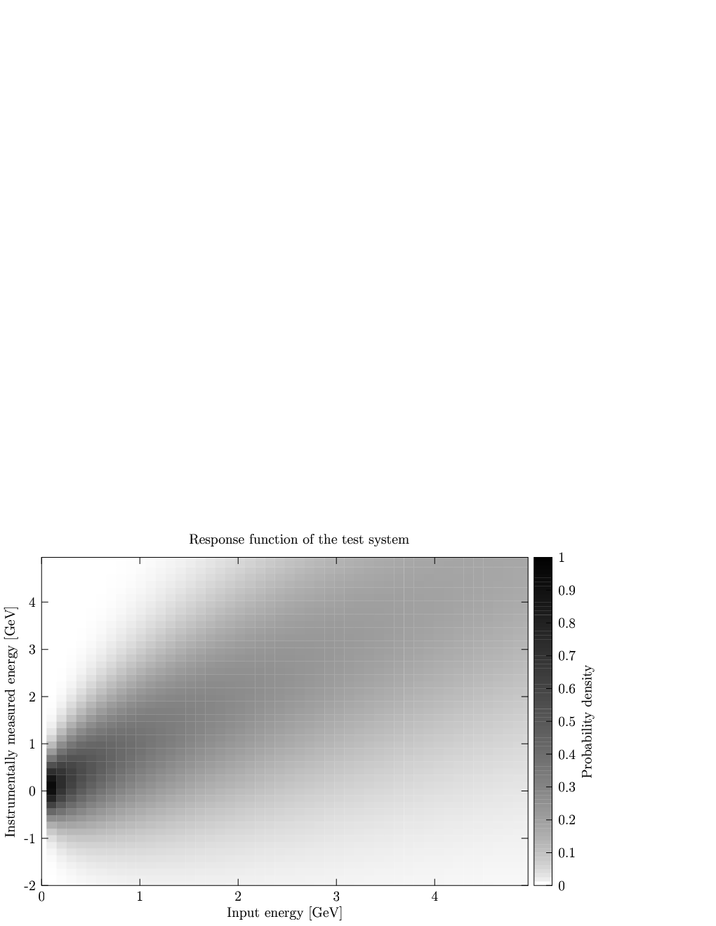
In this section the performance of the proposed method is illustrated on a numerical example. The example calculation is implemented via the C library libunfold [34], also including the automatic approximation, statistical and systematic error propagation formulae presented in the paper. The shown example is also shipped with the pertinent library. The illustrative case was deliberately chosen in a way when the response function is not translationally invariant, i.e. when ordinary deconvolution methods are not sufficient.

Our simulated measurement scenario is the following. We would like to measure the true pdf of a quantity, namely of the energy of produced charged particles in a high energy particle collision experiment. This true pdf used in our toy Monte Carlo shall be a parametrization of a real measurement at the LHC accelerator [35] at CERN. It is of the form

(115)

\displaystyle E

\displaystyle\mapsto

\displaystyle f(E):=\chi_{{}_{[0,\infty[}}(E)\;\;|E|\,\frac{(n-1)(n-2)}{(n\,T)^{2}}\,\left(1+\frac{|E|}{n\,T}\right)^{-n}

with parameters $n=6.6$ and $T=0.145\,\mathrm{GeV}$ . The response function

(116)

\displaystyle(E_{\mathrm{measured}},\,E_{\mathrm{true}})

\displaystyle\mapsto

\displaystyle\rho(E_{\mathrm{measured}}\,|\,E_{\mathrm{true}})

shall be such a cpdf that for each fixed value $E_{\mathrm{true}}>0$ the pdf

(117)

\displaystyle E_{\mathrm{measured}}

\displaystyle\mapsto

\displaystyle\rho(E_{\mathrm{measured}}\,|\,E_{\mathrm{true}})

shall be a Gaussian pdf with a mean of $E_{\mathrm{true}}$ and standard deviation of $a+\sqrt{b\,E_{\mathrm{true}}}+c\,E_{\mathrm{true}}$ , with parameter values $a=0.150\,\mathrm{GeV}$ , $b=0.7174\,\mathrm{GeV}$ , $c=0.074$ . This response function models the behavior of a calorimeter device used for the energy measurement of particles, namely of the HCAL calorimeter [36] of the CMS experiment at the LHC accelerator at CERN. In the simulated measurement scenario $10^{4}$ Monte Carlo samples according to the pdf Eq.(115) was generated, and its corresponding smeared response according to Eq.(116) was generated. These responses were assumed to be collected with an inefficiency of

(118)

\displaystyle E_{\mathrm{measured}}

\displaystyle\mapsto

\displaystyle\frac{1}{2}\left(1+\tanh\left(\frac{E_{\mathrm{measured}}-\mathcal{E}}{\Delta}\right)\right)\,d

with parameters $\mathcal{E}=1\,\mathrm{GeV}$ , $\Delta=1\,\mathrm{GeV}$ and $d=0.05$ , i.e. with an inefficiency not greater than $5\%$ on the overall measurement domain. The collected responses were histogramed, providing the measured pdf $g$ with our non-ideal detector. By construction, the statistical covariance matrix of the histogram $g$ shall be $\mathrm{diag}(g)$ . The inefficiency profile Eq.(118) causing a systematic deviation of the measured pdf from the folded pdf by Eq.(116), is assumed to be not known quantitatively and therefore is not corrected for. It is assumed, however, that an overall $5\%$ upper bound to this systematic deviation is known, being the systematic error of the measured pdf, i.e. one has $sg=0.05\,g$ . With these inputs, the linear iterative unfolding according to Eq.(10) was performed. The approximation errors were quantified using Remark 3.4 (vi). The propagated statistical errors were calculated according to Eq.(73). The propagated systematic errors were quantified using Theorem 7 (iii). The iteration was stopped when the combined statistical, approximation and systematic error exceeded a predefined threshold of $7\%$ . The result of the numerical test is shown in Fig. 1. Note, that more optimalized stopping criteria can also be invented, using the estimates for the approximation error, statistical error and systematic error. A natural candidate can be a double-threshold criterion: the approximation error needs to be below a threshold (sufficient shape restoration), whereas the combined statistical and systematic error must stay below an upper bound (divergence regularization). Also, the iteration might be stopped at the error optimum: at the minimum of the combined approximation, statistical and systematic error. Note, however, that one often might require a better shape reconstruction at the expense of increased statistical and systematic errors, as also seen in the shown example.

Refer to caption — Fig. 1: (Color online) Top left: illustration of the response function of our test example. The color intensity indicates the probability density of the response function. Top right: illustration of the unaccounted systematic distortion applied to the folded pdf in our test example. The solid curve indicates the systematic distortion (an inefficiency, in our example) on the unfolded pdf, which is assumed to be not exactly quantifiable, and therefore is not corrected for in the simulated measured pdf. Only an upper bound for the systematic distortion, called to be the systematic error, is assumed to be known for the simulated measured pdf. That is taken to be a constant $5\%$ upper bound in the example. Bottom left: the true input pdf (solid line), the simulated measured pdf (squares) and the unfolded pdf (triangles) by the proposed method. The pdfs are shown together with their bin-by-bin statistical errors (error bars), systematic errors (error bands), and approximation errors (narrow error bands). Bottom right: evolution of the bin-by-bin maximum of the approximation error (circles), statistical error (diamonds), and systematic error (flipped triangles) as a function of the number of iterations. Note that the binwise approximation errors converge to zero, but not in a monotonic manner, which explains the slight increase of that term after about $300$ iterations. If the iteration was continued, that term indeed converged to zero, but with several local minima, i.e. “waves” or “jumps” are seen in the convergence curve. On the other hand, the binwise statistical and systematic error term are seen simply to diverge, as expected. The competition of these three error terms gives a possibility to define a stopping criterion.

7 Concluding remarks

In this paper we presented mathematical proofs of convergence and error propagation formulae for a linear iterative unfolding method [1] in the probability theory context. It was shown that the pertinent method is convergent in the ‘binwise’ sense under quite generic conditions, which does hold in case of many practical applications. Furthermore, explicit formulae for the three important error terms, the approximation error, the statistical error and the systematic errors were derived. These can be used to define optimal iteration stopping criterion and quantification of errors therein. The key element of the proofs is the Riesz-Thorin theorem mapping the original $L^{1}$ problem to $L^{2}$ with a subsequent usage of spectral theory of $L^{2}$ operators. The typical use-cases of the method are those unfolding problems which cannot be handled by statistical deconvolution [9, 10], due to the absence of translational invariance of the response function. The possibility for propagation of the systematic errors is a special advantage, which deserves to be emphasized for experimental applications.

The pertinent method is also available as a C numerical library [34]. Using that, the method was demonstrated on a numerical example. The algorithm could be included in the ROOUnfold package [37] in the future, or in the GNU Scientific Library [38].

The present paper can serve also as a good motivation to perform similar convergence and error propagation studies on an other iterative unfolding method [18, 19, 21, 22, 23, 24, 25, 26], also called the method of convergent weights or iterative Bayesian unfolding. That method is non-linear and therefore is somewhat more complicated to study, however can be more suitable for unfolding problems in probability theory as it conserves the integral and non-negativity of probability density functions. Although widely used and numerically very promising, so far little is known on the convergence properties of that algorithm, and nothing is known about its error propagation. Our proposed method can be considered as the “linearized” version of that method, and thus the presented results are expected to provide clues also for the convergence and error propagation properties of the method of convergent weights or iterative Bayesian unfolding.

Acknowledgments

The author would like to thank to Tamás Matolcsi for valuable comments and for reading various versions of the manuscript, furthermore to Dezső Varga for discussions on the physical applications and on the relevance of error propagation formulae, in particular for the systematic errors. This work was supported in part by the Momentum (‘Lendület’) program of the Hungarian Academy of Sciences under the grant number LP2013-60. The author would also like to acknowledge the support of the János Bolyai Research Scholarship of the Hungarian Academy of Sciences.

References

[1] A. László: A linear iterative unfolding method. J. Phys. Conf. Ser. 368 (2012), 012043.
[2] A. László: A robust iterative unfolding method for signal processing. J. Phys. A39 (2006), 13621. Zbl 1107.94004
[3] G. Cowan: Proceedings of Conference on Advanced Statistical Techniques in Particle Physics (18-22 March 2002, Durham, United Kingdom) (2002, IPPP/02/39, Durham) p 248
[4] V. Blobel: Unfolding for HEP Experiments (Talk at DESY Computing Seminar, 2008) http://www.desy.de/˜blobel/DESYcompsem08.pdf
[5] G. Bohm, G. Zech: Introduction to Statistics and Data Analysis for Physicists (2010, Hamburg: Verlag Deutsches Elektronen-Synchrotron).
[6] M. Kuusela, V. M. Panaretos: Statistical unfolding of elementary particle spectra: empirical Bayes estimation and bias-corrected uncertainty quantification. Ann. Appl. Stat. 9 (2015), 1671.
[7] M. Kuusela, P. B. Stark: Shape-constrained uncertainty quantification in unfolding steeply falling elementary particle spectra. Preprint (2016) [arXiv:1512.00905].
[8] H. P. Dembinski, M. Roth: An algorithm for automatic unfolding of one-dimensional distributions. Nucl. Instr. Meth. A729 (2013), 410.
[9] I. Dattner, A. Goldenshluger, A. Juditsky: On deconvolution of distribution functions. Ann. Stat. 39 (2011), 2477. Zbl 1232.62056
[10] I. Dattner, M. Reiß, M. Trabs: Adaptive quantile estimation in deconvolution with unknown error distribution. Bernoulli 22 (2016), 143. Zbl 06543266
[11] J. Fan: On the optimal rates of convergence for nonparametric deconvolution problems. Annals of Stat. 19 (1991), 1257. Zbl 0729.62033
[12] C. H. Hesse: Iterative density estimation from contaminated observations. Metrika 64 (2006), 151. Zbl 1100.62042
[13] F. Comte, C. Lacour: Anisotropic adaptive kernel deconvolution. Ann. Inst. H. Poincaré Prob. Stat. 49 (2013), 569. Zbl 06171260
[14] M. C. Liu, R. L. Taylor: A consistent nonparametric density estimator for the deconvolution problem. Can. J. Stat. 17 (1989), 427. Zbl 0694.62017
[15] L. A. Stefanski, R. J. Carol: Deconvoluting kernel density estimators. Statistics 21 (1990), 169. Zbl 0697.62035
[16] J. Kalifa, B. Rouge: Deconvolution by Thresholding in Mirror Wavelet Bases. IEEE Trans. on Image Proc. 12 (2003), 446.
[17] A. Hoecker, V. Kartvelishvili: SVD Approach to data unfolding. Nucl. Instr. Meth. A372 (1996), 469.
[18] G. D’Agostini: A multidimensional unfolding method based on Bayes’ theorem. Nucl. Instr. Meth. A362 (1995), 487.
[19] G. Zech: Iterative unfolding with the Richardson-Lucy algorithm. Nucl. Instr. Meth. A716 (2013), 1.
[20] C. Alt et al: High Transverse Momentum Hadron Spectra at $\sqrt{s_{{}_{NN}}}=17.3\,\mathrm{GeV}$ , in Pb+Pb and p+p Collisions. Phys. Rev. C77 (2008), 034906.
[21] W. H. Richardson: Bayesian-based iterative method of image restoration. J. Opt. Soc. of Amer. A62 (1972), 55.
[22] L. B. Lucy: An iterative technique for the rectification of observed distributions. Astronomical Journal 79 (1974), 745.
[23] L. A. Shepp, Y. Vardi: Maximum likelihood reconstruction for emission tomography. IEEE Trans. Med. Imag. 1 (1982), 113.
[24] A. Kondor: Method of convergent weights – An iterative procedure for solving Fredholm’s integral equations of the first kind. Nucl. Instr. Meth. 216 (1983), 177.
[25] H. N. Mülthei, B. Schorr: On an iterative method for a class of integral equations of the first kind. Math. Meth. Appl. Sci. 9 (1987), 137. Zbl 0628.65130
[26] H. N. Mülthei, B. Schorr: On an iterative method for the unfolding of spectra. Nucl. Instr. Meth. A257 (1987), 371.
[27] P. D. Lax: Functional analysis (2002, Chichester: Wiley-Interscience). Zbl 1009.47001
[28] W. Rudin: Functional Analysis (1973, New York: McGraw-Hill). Zbl 0253.46001
[29] G. Arfken: Fourier Convolution theorem 20.4 Mathematical Methods for Physicists 7rd edn (2013, Amsterdam: Elsevier/Academic Press) pp 985. Zbl 1239.00005
[30] P. Bracewell: Convolution theorem The Fourier Transform and Its Applications 3rd edn (1999, New York: McGraw-Hill) pp 108.
[31] L. Landweber: An iteration formula for Fredholm integral equations of the first kind. Am. J. Math. 73 (1951), 615. Zbl 0043.10602
[32] G. B. Folland: Real Analysis: Modern Techniques and Their Applications 2nd edn (1999, Wiley-Interscience). Zbl 0924.28001
[33] N. Dinculeanu: Vector Measures (1967, Elsevier). Zbl 0142.10502
[34] A. László: The libunfold package (2011, Source code)
http://www.rmki.kfki.hu/˜laszloa/downloads/libunfold.tar.gz
[35] V. Khachatryan et al (the CMS collaboration): Transverse-Momentum and Pseudorapidity Distributions of Charged Hadrons in pp Collisions at $\sqrt{s}=7$ TeV. Phys. Rev. Lett. 105 (2010), 022002.
[36] E. Yazgan (for the CMS collaboration): The CMS barrel calorimeter response to particle beams from 2 to 350 GeV/c. J. Phys. Conf. Ser. 160 (2009), 012056.
[37] T. Adye et al: The ROOUnfold package
http://hepunx.rl.ac.uk/˜adye/software/unfold/RooUnfold.html
[38] The GNU Scientific Library: http://www.gnu.org/software/gsl