Calculating Casimir interactions for Periodic Surface Relief Gratings using the C-Method
Abstract
We develop a formalism to calculate the fluctuation-induced interactions in periodic systems. The formalism, which combines the scattering theory with the C method borrowed from electromagnetic gratings studies, is suitable and efficient for the calculation of the Casimir forces involving surface relief gratings. We apply the developed technique to obtain the energy and lateral force for simple 1-D sinusoidal gratings. Using this formalism we derived known asymptotic expressions that were previously obtained through perturbative approximations. At close separation, our numerical results match those obtained by the proximity force approximation and its first correction using the derivative expansion.
Keywords:
QED corrections to long-range and weak interactions, Gratingspacs
31.30.jh,42.79.DjI Introduction
In a seminal paper in 1948, H. G. B. Casimir [1] found the presence of an attractive interaction between two neutral perfect mirrors in vacuum. This effect was later generalized to real materials (finite conductors and dielectrics) by E. M. Lifshitz[2], which has some consequences for micro and nano-scale mechanical devices, often leading to a very strong attraction between parts called stiction[3, 4]. To this end, a complete quantitative understanding of the Casimir effect is necessary for the proper design and analysis of MEMS and NEMS. The goal is to be able to exert some control over the Casimir forces by manipulating the material or geometry of the system.
There have been a number of experiments showing that the magnitude of the Casimir force could be varied by changing the surface geometry of the interacting objects [5, 6, 7, 8, 9, 10, 11, 12, 13, 14]. To investigate the impact of curvature and corrugation, the Casimir forces have been measured between a sphere and a sinusoidal grating [5] and between two corrugated surfaces for both aligned [6, 7] and crossed [13, 14] corrugations.
Until recently most of the theoretical analysis of the Casimir force experiments has been done using the proximity force approximation (PFA), also known as the Derjaguin approximation [15] for which the curved surfaces are assumed to be made up of infinitesimal finite plates. Using this approximation, one can calculate the force (or energy) between curved objects through the expression for infinite parallel plates. This approximation is only valid in the limit as the separation is much smaller than the radius of curvature of the curved surfaces. As the experiments have become more sensitive, it has become necessary to do the theoretical analysis outside the range of validity of the PFA. Recently a derivative expansion (DE) approach has been introduced [16, 17, 18], which reproduces the PFA and gives the next order correction, and which has successfully explained a number of new recent experiments [13, 14]. The first theoretical calculation of the Casimir force between geometrically patterned surfaces not using the PFA was reported in 2001 [19, 20], which described the normal and lateral forces between two aligned corrugated surfaces in terms of a perturbative expansion in the profile height. Since then, this perturbative approach has been expanded to include real material properties and unaligned corrugations [21, 22, 23, 24, 25]. More recently the scattering method has been used to obtain the Casimir forces in periodic systems [26, 27, 28]. For example in Ref. [27], the scattering method along with rigorous coupled wave analysis (RCWA), an approach developed for electromagnetic grating theory, is used to calculate the Casimir forces in the Corrugated systems.
In this paper, we combine the scattering theory with the C method, an efficient technique for calculating the Rayleigh coefficients optimized for surface relief gratings [29, 30, 31, 32]. We note that for smooth height profiles (such as a sinusoidal grating) the C method has some significant advantages over the RCWA. The RCWA assumes that the system is made up layers with square sides, and many layers are required to accuratly model smooth surface profiles. In Ref. [33] the C method was compared to the RCWA for sinusoidal gratings, and it was found that 40 layers were required in the RCWA to match the same accuracy from the C method. With 40 layers, the calculation employing the RCWA was much slower than that using the C method. It should be noted that for rectangular gratings the RCWA would perform much better than the C method. This method is not meant to replace the RCWA, only complement it by describing a method appropriate for smoothly varying surfaces.
The structure of the paper is as follows. While Sect. II briefly describes the scattering method, and explicitly gives the basis functions and the translation matrix, Sect. III describes the C method. In Sec. IV the C method is used to perturbatively calculate the Casimir energy as a power series in the profile height. Section V describes in detail the numerical algorithm used to calculate Casimir quantities. In Sec. VI the numerical results are explored and compared to the PFA and its first correction using the DE approach, and the perturbative approximation. A summary of the work and its main conclusions are presented in Sec. VII. Details of our calculations are relegated to the appendix.
II Scattering Formalism for the Casimir Energy
The scattering method has been extensively used for the calculation of the Casimir forces between the objects with different geometries and material properties. In this paper, we use the scattering method to find the Casimir energy between two planes with a periodic structure. The method can be easily extended to periodic structures. In general, the Casimir free energy between two objects at the temperature T is given by
| (1) |
with the translation matrix and the scattering matrices of the objects. Both the translation and scattering matrices depend upon the imaginary Matsubara frequencies
| (2) |
From Eq. (1) for the energy, the Casimir forces or torques between two objects can be calculated by taking derivatives. Indeed, the scattering method simplifies the fluctuation-induced problems by separating the calculation into finding the translation matrices () and scattering matrices (). The matrix corresponds to the way the fluctuations propagate through the field between the objects and the -matrix represents the interaction of the object with the fluctuations. Thus the information about the distance between the objects is only contained in the translation matrices. The elements of the translation and scattering matrices are generally calculated in a coordinate system appropriate to the geometry of an object. In the next section we present the vector basis function suitable for a corrugated system.
II.1 Vector Basis Functions
For a periodic system the obvious choice of the vector basis functions are Block-periodic plane waves
| (3a) | ||||
| (3b) | ||||
with the vector a constant vector known as a pilot vector and solutions to the scalar Helmholtz equation,
| (4) |
which are
| (5) |
These basis functions are recognizable as the simple plane wave vector functions where the transverse wave-vector has been replaced with the Block wave-vector . The block wave-vector can be written as
| (6) |
with a continuous wave-vector that only takes on values in the first Brillouin zone and a discrete lattice vector given by
| (7) |
where and are inverse lattice vectors of the periodic system, and and are integers. Using the aforementioned basis, we can now define the translation and scattering matrices.
II.2 Translation Matrix
Because the vector basis functions are essentially plane waves, the translation matrix is simply
| (8) |
with a in plane displacement, and a perpendicular separation. It should be noted that for a fixed separation , the matrix is exponentially suppressed for large imaginary frequency . In addition for fixed separation and fixed imaginary frequency , the elements of the translation matrix are exponentially suppressed in and . Both of these features are needed for the Casimir quantities to converge (both in the frequency integral, and as a function of matrix size) and for making the evaluation of relevant matrices numerically efficient.
II.3 Scattering Matrix

To obtain the scattering matrix, we divide the space into three regions as illustrated in Fig. 1: region completely above the periodic surface, region completely below the periodic surface, and region including the periodic surface. We now consider an incident wave () is scattered by the surface in region , and is either reflected back into region or transmitted into region
| (9) |
The reflected or transmitted field can be written as a sum over the complete set of vector basis functions. Furthermore because of the boundary conditions at infinity the reflected wave in region only contains exponentially dying wave and the transmitted wave in region only contains exponentially growing waves (dying in the negative direction). Because the system is periodic, the Floquet-Bloch theorem states that the solution must be pseudo-periodic (periodic with a phase factor). The reflected and transmitted fields can then be completely written as
| (10a) | ||||
| (10b) | ||||
This is known as the Rayleigh expansion with the matrix elements of the and matrices called the Rayleigh coefficients.
For the remainder of this work many simplifications will be performed to make the derivations more tractable, and the results easier to analyze. We will consider a two parallel 1-D periodic systems alligned along the axis of corrugations made of perfectly conducting materials at zero temperature.
II.4 1-D corrugation perfect metal at zero temperature
We consider 1-D corrugations that are translationally invariant in the direction. A natural direction for the pilot vector in Eqs. (3) is then . The full electric field can then be rewritten in terms of two scalar fields, the TM and TE modes defined as
| (11a) | ||||
| (11b) | ||||
where both fields satisfy the Helmholtz equation
| (12) |
with . The scattering problem can be written
| (13) |
where the incident wave is the Fourier transform of scalar basis function in Eq. (5)
| (14) |
For perfect electrical conductors the boundary conditions reduce to Dirichlet and Neumann boundary conditions,
| (15a) | ||||
| (15b) | ||||
The zero temperature condition will change the sum over Matsubara frequencies given in Eq. (1) to an integral over imaginary frequency. The Casimir energy per unit length between two 1-D perfect metal corrugations can then be written as
| (16) |
where the sum over the polarization contains the TE and TM modes. To calculate the Casimir energy using Eq. (16), we need to find the scattering matrix that we obtain in the next section using the C-method.
III C-Method
The C method was developed as an efficient numerical method for calculating the Rayleigh coefficients for surface relief gratings [29]. In this section, we describe the C method for simple 1-D perfectly conducting boundary conditions. For other boundary conditions see Ref. [31] and references therein. In what follows we present the C method for the corrugated system, which involves an explicit change of variable to remove the dependence, the direction perpendicular to the mean surface of grating, followed by a Fourier transform in the and coordinates. This procedure expresses the Helmholtz equation, Eq. 4, as a quadratic eigenvalue problem more amenable to numerical solutions.
We start with the following change of variable
| (17) |
While this change of variable will have the effect of explicitly removing the dependence from the boundary condition, it will introduce the gradient of the profile function into the Helmholtz equation through the partial derivatives
| (18) |
In the next step, we write the profile function and the fields in a Fourier series
| (19a) | ||||
| (19b) | ||||
where and are the inverse lattice and Block vectors defined in Eq. (6). For the 1-Dimensional periodic profiles considered the vectors can be explicitly written
| (20) |
where is the period of the profile. The partial derivatives of based on Eqs. (18) and (19) then yield
| (21) |
and
| (22) |
By combining , and changing the variable , Eq. (22) becomes
| (23) |
Using Eq. (21) and (23), Eq. (18) can be written in the following compact form
| (24) |
such that
| (25a) | ||||
| and and are matrices with elements defined by | ||||
| (25b) | ||||
| (25c) | ||||
Separating out the Fourier modes, the Helmholtz equation can now be written as an infinite system of ordinary differential equations
| (26) |
whose solution is assumed to have an exponential form
| (27) |
with eigenvalue and eigenvector . Upon substitution of Eq. (27) into Eq. (26), we obtain a quadratic eigenvalue problem for the eigenvalues and eigenvectors,
| (28) |
with
| (29a) | ||||
| (29b) | ||||
| (29c) | ||||
The general solution to the full wave equation can now be written by combining Eqs. (19b), (25a), and (27)
| (30) |
with indexing the solutions to the quadratic eigenvalue problem, and undetermined coefficients. The undetermined coefficients can be found by applying the boundary conditions given in (15).
III.1 Boundary Conditions
To apply the boundary conditions in Eqs. (15) to the total field
| (31) |
we need to write the incident and reflected waves in a Bloch series.
The incident wave is simply an exponentially growing (dying in the negative direction) plane wave basis function indexed by . After a change in variables to the coordinates, the plane wave can be written
| (32) |
with the Rayleigh wavenumber
| (33) |
Note the change in variable introduces an additional dependence such that Eq. (32) is not strictly a Fourier series in . However, we can still expand the incident wave in a Fourier series
| (34) |
where the term are the Fourier coefficients,
| (35) |
Further, the reflected wave can be written as in Eq. (30) in terms of the eigenvalues and eigenvectors of the quadratic eigenvalue problem
| (36) |
It should be noted that because the reflected wave must go to zero in the limit we need only to use the set of eigenvalues and their associated eigenvectors. The quantity in Eq. (36) corresponds to the Fourier index of the incident wave, and the index labels the mode as either TM or TE.
Now, inserting Eqs. (34) and (36) in the boundary condition Eqs. (15a) and (15b), and separating out the modes, we find a system of equations for the unknown coefficients written in matrix form as
| (37) |
where and are given explicitly for the TM and TE modes below.
For the TM mode, the total field at obeys Dirichlet boundary conditions
| (38) |
In this case the matrix is simply the matrix of eigenvectors
| (39) |
and the vectors are simply the Fourier coefficients of the incident wave
| (40) |
The TE mode obeys Neumann boundary conditions given in Eq. (15b). In the coordinates Eq. (15b) becomes
| (41) |
with the first derivative of the profile function with respect to . After separating out the Fourier modes, the matrix is
| (42) |
and the vector is
| (43) |
with matrices , , and the vector defined in Eqs (25b),(25c), and (35), respectively. Utilizing these expressions it is possible to solve for the unknown coefficients , which in turn gives the exact form of the field for the scattering problem.
III.2 Identifying Rayleigh Coefficients
In order to find the Rayleigh coefficients we must compare the expression for the reflected wave in Eq. (36) to that in region using the Rayleigh expansion as given in Eq. (10). An expansion analogous to Eq. (10) for a 1-D corrugations in the coordinate system yields
| (44) |
Using the Fourier expansion of the basis functions as given in Eq. (34), we write the full reflected wave in Eq. (44) as
| (45) |
with the Rayleigh wavenumber defined in Eq. (33) and the Fourier coefficients of the incident wave given in Eq. (35).
Equation (45) corresponds to the Rayleigh expansion in the coordinates. The Rayleigh coefficients can be obtained by matching Eq. (30) with Eq. (45) term by term,
| (46) |
where is the index of the eigenvalue that matches with the Fourier index. Note that the eigenvectors and eigenvalues are determined by the quadratic eigenvalue problem in Eq. (28). The coefficients are determined by solving the linear system in Eq. (37). Equations (28), (37), and (46) can be used to numerically calculate the Rayleigh coefficients, and through them the Casimir energy. However, it is possible to obtain analytical results in certain limits, which we present in the next section.
IV Small Amplitude Perturbation
In the limit of small amplitude surface relief gratings, perturbation theory can be used to analytically obtain the Casimir energy as a series in the height profile . Using the C method we can obtain a perturbative expression for the Rayleigh coefficients , which requires perturbative expressions for the eigenvectors and eigenvalues .
Solving the quadratic eigenvalue problem given in Eq. (28) perturbatively, we expand the matrices and up to the order and respectively. In addition, we set the eigenvalues and eigenvectors , where the term is of order . Grouping the terms together by powers of , we find the zeroth order equation
| (47) |
The matrix is diagonal and thus the eigenvectors are given by Kronecker delta functions, . The eigenvalues are the square root of the diagonal elements of the matrix. In order to get the exponentially dying components, we consider only the negative eigenvalues
| (48) |
This is the same as the negative Rayleigh wavenumber given by Eq. (33). To the zeroth order, the reflected waves are just plane waves.
The first two corrections to the eigenvalues are
| (49) | ||||
| (50) |
The derivations of Eqs. (49) and (50) are given in Appendix (A.1). The careful examination of Eq. (50) shows that the sum is exactly zero for and very small for near zero. Note that the term is exactly zero for and for , is even in around while odd. Thus, the sum of the and terms is exactly zero. For finite matrices where ranges from to the cancellation will only occur exactly for . For near zero, if then most of the terms will cancel, leaving terms where . If the Fourier coefficients decay fast enough then the second order correction is negligible for near 0.
The first and second order corrections to the zeroth order eigenvectors are
| (51) | ||||
| (52) |
Similar to the situation with the second order eigenvalues, the second term in Eq. (52) can be shown to be negligible for near zero.
We now use Eqs. (37) and (46) to find a perturbative expansion for the Rayleigh coefficients. The expressions for the matrices in Eq. (37) can be found using the perturbative expansions for the eigenvalues and eigenvectors in Eqs. (39) and (42). However we still need a pertubative expansion for the term used in Eqs. (40), (43), and (46). The terms are the Fourier coefficients of an incident (+) or a scattered (-) plane wave in the coordinate system. Using a series expansion in powers of the height profile , , each term can be identified as the Fourier coefficients of powers of the profile function given in Eq. (35). The first three terms are
| (53a) | ||||
| (53b) | ||||
| (53c) | ||||
It should be noted that the zeroth, first, and second order expansions of the eigenvectors in the perturbative expansion exactly match with the first three terms of a perturbative expansion of the plane wave in the coordinate system given by Eq. (34). From this expansion it is possible to make the identification
| (54) |
through second order. Note that the zeroth order eigenvalue is exactly equal to the Rayleigh wavenumber for the plane wave as given in Eq. (48), and the first two corrections are zero, see Eqs. (49) and (50).
The equality in equation (54) between the basis functions identified through the C-method and simple plane waves seems to imply the Rayleigh hypothesis, which consider the solution to the scattering problem can be written in terms of only the exponentially dying waves even inside the grooves in region . Note that in Refs. [34, 35] it is shown that the Rayleigh hypothesis is valid for certain profiles with small enough height amplitudes. We emphasize that the perturbative expansion presented in this section is performed under the assumption that the maximum profile height is smaller than all other length scales in the system. Thus we expect that the equality presented in Eq. (54) would be true to all orders.
Inserting Eq. (54) into Eq. (46), we find the Rayleigh coefficients are exactly given by the undetermined coefficients . Using the perturbative expressions for the eigenvalues and eigenvectors, Eqs.(48)-(52), it is possible to solve Eq. (37) perturbatively for the Rayleigh coefficients. The expressions for the modes are
| (55a) | ||||
| (55b) | ||||
| (55c) | ||||
and for modes are
| (56a) | ||||
| (56b) | ||||
| (56c) | ||||
where the is a modified Rayleigh wave-vector given explicitly as
| (57) |
A more detailed derivation of Rayleigh coefficients is presented in Appendix A.2.
Inserting Eqs. (55) and (56) into Eq. (1), we can obtain the perturbative expansion for the Casimir energy in powers of the grating profile . For a single grating above a flat sheet, the zeroth order term gives the expression for the Casimir energy between two parallel plates, which is expected as the zeroth order reflection coefficients correspond to those for flat plates. The first order correction is
| (58) |
with the zeroth Fourier mode of the height profile, also the average height of the grating. Equation 58 is equal to zero if we define the profile to have zero average height (such as a sinusoidal grating). The second order correction to the energy is
| (59) |
where the and are integral expressions given explicitly in Eqs. 95 in App. A.3. The complete details of the derivation of perturbative energies and the lateral Casimir forces are given in App. A.3. It is important to note that the expressions for the energy and lateral force given in Eqs. (59) and (99) exactly match the previous results obtained in Refs. [19, 20, 24, 25].
V Numerical Method
Here we employ the C method described in previous sections to calculate the Casimir energy through Eq. (16). The integrand in Eq. (16) depends on the height profile or its Fourier components , the combined wave-vector , the wave-vector in the direction , and the maximum Forier mode . All the relevant matrices will then be of size , with . As an example we assume a sinusoidal profile with . To obtain eigenvalue eigenvector pairs presented in Eq. (28), we need to generate matrices , , and . For the sinusoidal profile function the Fourier components are trivially found, . The matrix elements of the matrix (see Eqs. (20) and (25c)) are
| (60) |
from which we can find
| (61) | ||||
| (62) | ||||
| (63) |
For a given , and a finite matrix, the quadratic eigenvalue problem in Eq. (28) will yield eigenvalues and eigenvectors that can be obtained numerically. The standard method is to recast the quadratic eigenvalue problem into a larger (generalized) eigenvalue problem with a matrix given in block form as
| (64) |
where we can identify the vector as constructed from block components of and . The eigenvalues and eigenvectors for the generalized eigenvalue problem in Eq. (64) are found numerically, and the first components of the eigenvector are the same as the components of the eigenvector of the corresponding quadratic eigenvalue problem. We sort the eigenvalue, eigenvector pairs into those with eigenvalues with positive real part , and with negative real parts . We label the negative pairs with an index that will run from 1 to . Figure 2 shows a scatter plot of the numerically obtained eigenvalues (circles) on the complex plane. Using the eigenvalue and eigenvector pairs and Eqs. (39) and (42), we are now able to generate the and . Our goal is solve to the matrix equation given in Eq. (37) for both - and -polarizations to obtain the coefficients which later will be used to obtain the Rayleigh coefficients.
The target vectors and given in Eqs. (40) and (43) both depend on the term, Eq. (35). For the sinusoidal profile, the term can be evaluated as
| (65) |
with the order modified Bessel functions of the first kind. Substituting and in Eq. (37), we construct an matrix of the coefficients with indices and . The index corresponds to the Fourier index, and runs from to . The index corresponds to the index of the eigenvalue and runs from to .

It is now possible to obtain the Rayleigh coefficients from the ones by comparing Eq. (30) and (45). We can identify the Rayleigh coefficients as proportional to the coefficients only if the eigenvalue matches the Rayleigh wavenumber . It should be noted, as mentioned in Sec. IV, that the eigenvalue will perfectly match the Rayleigh wavenumber only in the limit of inifinitely large matrices. As is shown in Eq. (50), only a subset of the indexed eigenvalues will match with the Rayleigh wavenumbers for finite matrices. Specifically the subset will match the Rayleigh wavenumbers that correspond to Fourier modes with near zero. This is clearly illustrated in the example given in Fig. 2. In this example, only the first 11 eigenvalues (circles) matched Rayleigh wavenumbers (crosses). In practice, we consider that any eigenvalue matched a Rayleigh wavenumber when relative difference between them was below some tolerance (). We need to identify the pairs for which . For the example given in Fig. 2, these are = (1,0), (2,-1), (3,1), (4,-2), (5,2), etc. These matched pairs, along with the coefficients, the eigenvectors , and the terms are used in Eq. (46) to find the Rayleigh coefficients for and . In the example, we would only keep scattering coefficients for and between and as only the first 11 eigenvalues matched with the Rayleigh wavenumbers.
In addition to Rayleigh coefficients , we need to obtain through Eq. (8) in order to calculate the integrand given in Eq. (1). To obtain the Casimir energy, we then numerically integrate over wave-vectors and for a fixed maximum Fourier mode size . All the relevant matrices are calculated for Fourier modes, running from to . The maximum Fourier mode is steadily increased from until the Casimir quantity of interest has converged. For the purposes of this paper a Casimir quantity is defined as converged when the relative change in the quantity when increasing by five is less than .
VI Results


We now use the numerical method presented in the previous section to calculate the energy and lateral force for two systems shown in Figs. 4 and 4. We calculate the Casimir energy in the simplest system possible: a flat plate separated from a sinusoidal grating (Fig. 4), and the lateral Casimir force for the simplest system exhibiting a non-zero lateral force: two identical sinusoidal gratings (Fig. 4). The average separation distance between two plates in both systems is . The sinusoidal gratings have an amplitude and a wavelength as described in Figs. 4 and 4.

For the energy calculations, there are two dimensionless parameters, the amplitude over the wavelength and the mean separation over the wavelength. The Casimir energy is calculated for values of from 0 to (at which point the corrugations would contact the planar surface) and for values of ranging from to . For the purpose of this paper, we increased the value of the maximum Fourier mode from 1 up to 30 for the convergence of the Casimir energy. The Casimir energy converged for for is less than 0.0575, 0.135, 0.4, 0.7, 1.2, 2.75 for values of 0.1, 0.2, 0.5, 1, 2, 5 respectively.
For all tested values of the larger values of did not converge for the maximum Fourier nodes . It would be possible to increase the range of convergence by choosing larger values of , at the cost of a longer computational time. The lighter shaded (red online) region in Fig. 5 illustrates the approximate parameter space in which the Casimir calculation using the C method converges. The dashed (red) line is an empirical fit of the data to a rightward facing parabola. The first obvious feature in the figure is that if then the corrugations touch and pass through the flat plate, an unphysical situation. This is shown in the figure by the dark gray overlap region. The horizontal and vertical hashed regions correspond to the regions of validity of the analytical methods corresponding to the proximity force approximation with derivative expansion and the perturbative expansion which we will discuss in the next two sections, respectively.
A quick note should be stated about the computational expense of the Casimir calculations using the C method. All numerics were programmed in Wolfram Mathematica, on a modern desktop (2.8 GHz 64 bit processor, with 8 GB ram). A single energy or lateral force calculation takes about 100 cpu seconds for and about 900 cpu seconds ( 15min) for . The computational cost appears to scale with for the range of from 1 to 30.
VI.1 Comparison with PFA and Derivative Expansion
The graphs in Fig. 6 show the comparison of the numerical calculations using the C method to the analytic results, obtained as
| (66) |
with the PFA energy obtained by assuming that the curved surfaces are made up of infinitesimal parallel plates and summing over the contribution of all the plates. The PFA approximation for the Casimir energy per unit area for a sinusoidal grating as shown in Fig. 4 is
| (67) |
The PFA is a valid approximation if the radius of curvature of objects is large compared to the separation distance between the objects. For our systems, this translates into the condition , given by the horizontally hashed region in Fig. 5.
The quantity in Eq. (66) corresponds to the derivative expansion (DE) introduced in Ref. [16] for scalar fields and Refs. [17, 18] for electric fields with perfect conductor or dielectric boundaries. The first correction for the energy per unit area per mode is
| (68) |
where indexes the polarization (TM or TE) and is a constant given as and .
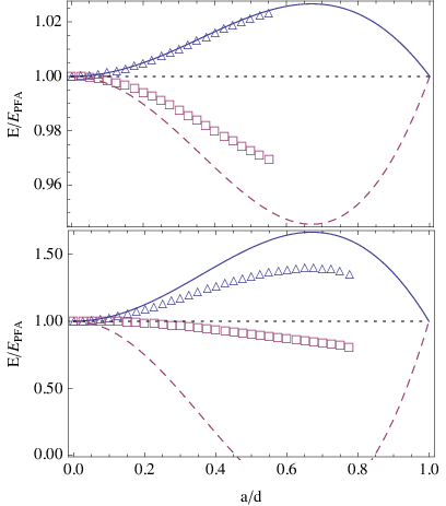
The graphs in Fig. 6 show the Casimir energy normalized to the PFA vs , with running form 0 to 1 and for two different values of . The two curves in Fig. 6 correspond a vertical trace in the parameter space in Fig. 5. The approximations should be exact at the two limits of and , related to a flat plate and the tips of the corrugations touching the flat surface, respectively. The upper graph is for the small fixed value , where it is expected that the PFA+DE approximations be fairly accurate over the entire separation. The TM mode shows very good agreement over the region of convergence. The DE for the TE mode seems to overestimate the correction for this separation. The lower graph is for a larger fixed value of . For this separation the DE seems to overestimate the correction to the PFA for both the TM and TE modes over most of the range of convergence. It should be noted that the numerical results for the TM mode show the beginning of a downward turn as is increased.

The graphs in Fig. 7 show the lateral Casimir force versus the lateral displacement for a fixed separation and amplitude . The values of the mean separation and amplitude were chosen to show the range of applicability of the scattering technique using the C method. The small value of the mean separation ensures the validity of PFA+DE approximations, allowing a good benchmark to be compared with our results. The larger relative value of should ensure that the force is far from purely sinusoidal. The graph in Fig. 7 shows good agreement between the numerical results and the analytic PFA+DE for both the TM and TE modes, and is far from sinusoidal. For larger separations and larger amplitudes the PFA+DE grossly overestimates the magnitude of the lateral Casimir force.
VI.2 Comparison with Perturbative Calculations
This section compares the perturbative approximation derived in section IV to the numerical results. The perturbative expansion results are obtained under the assumptions that and . The region of validity for the perturbative approximation is shown by the vertically hashed region in Fig. 5.
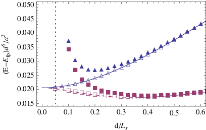
A comparison of the perturbative expansion with the numerical calculation using the C method is presented in Fig. 8. The empty triangles are for a fixed small value of , which traces a diagonal line in Fig. 5. As shown in Fig. 8, for this small value of the perturbative expansion should be valid over the entire range of separations. The filled triangles are for a fixed value of , which traces a horizontal line in Fig. 5. As shown in Fig. 8, for fixed profile heights the perturbative expansion breaks down and severly underestimates the energy for short separations. The deviation of the numerical results from the perturbative expressions becomes apparent for small values of as expected.

The graph in Fig. 9 illustrates a comparison of the perturbative expansion results with the numerical calculation for the lateral Casimir force. The calculation is done for a larger value of mean separation and a smaller value of the amplitude . In this region of parameter space one expects the perturbative expansion to be still valid, while the PFA begins to fail. The graph shows good agreement with the perturbative approximation for both TM (triangles) and TE (squares) modes. The dashed line represents the next to leading order expansion as calculated in Refs. [24]. For larger amplitudes, the perturbative expansion dramatically underestimates the lateral Casimir force, not shown in the figure.
VII Conclusion
In general, it is difficult to calculate the Casimir energy between non-planar surfaces, and the analytical approximations used such as PFA, the derivative expansion, and perturbative expansions in the profile height are all valid in a small region of the parameter space, see Fig. 5. In this paper, we combined the scattering theory with the C method, a powerful technique borrowed from electromagnetic grating theory, to calculate the Casimir energy for surface relief gratings.
The C method is in particular suitable for calculating the scattering matrices for smoothly varying height profiles, which allows us to obtain the Casimir energy over a wider range of phase space than that accessible by the analytic approximations. Figure 5 shows the region of convergence of C method when we kept the size of our relevant matrices relatively small. Each point obtained in the plots of Figs. 6, 7, 8, and 9 was produced using a desktop computer for 900 cpu seconds. One can easily expand the region of convergence by increasing the size of matrices and allocating more CPU time. The limiting factor will then become the roundoff error inherent to the solution of the system of equations given in (37). This issue has been addressed in Ref. [32] along with an alternative method for solving the system of equations that improves numerical stability.
It is important to note that the scattering method has been previously used to calculate the Casimir interactions for surface relief gratings using a small amplitude perturbation series for the reflection coefficients[21, 22, 23]. We emphasize that in all previous work, in order to find the perturbative corrections to the reflection coefficients the Rayleigh hypothesis was assumed. In addition to the scattering approach, other techniques were employed to calculate the Casimir forces for perfect materials[19, 20, 24, 25]. These calculations were also done under the assumption of the Rayleigh hypothesis. In this paper, we performed all the calculations without assuming the Rayleigh hypothesis and showed that the perturbative calculations implicitly make such an assumption.
We compared the numerical results of this paper against known analytic approximations: the PFA plus the first correction to the PFA using the derivative expansion and the perturbative expansion and found very good agreement in the regions of parameter space where the approximations are expected to be valid.
The method presented in the paper can be easily extended beyond the perfectly conducting case to include general dielectrics, and is valuable tool to employ in understanding the Casimir force for surface relief gratings.
Acknowledgments
The authors would like to thank Alex Banishev, Umar Mohideen, Ehsan Noruzifar, Thorsten Emig, and Mehran Kardar, Kim Milton, Prachi Parashar, and Elom Abalo for helpful discussions. JW thanks Stephen Fulling for the invitation to present this work at Texas A&M. This work was supported by DMR-1310687.
Appendix A Perturbative Calculation
The appendix provides some of the details of the derivations of the perturbative results found in the Sec. IV. The goal is to find an analytic approximation for the Casimir energy or lateral Casimir force for surface relief gratings. The Casimir energy and lateral Casimir force depend upon the Rayleigh coefficients, which in turn depend upon the eigenvectors and eigenvalues of the quadratic eigenvalue problem given in Eq. (28). This section will cover the results in the order they are needed in the body of the paper: First we expand the eigenvectors and eigenvalues, second the Rayleigh coefficients, and finally the Casimir energy and lateral Casimir force up to the second order in the amplitude of height profile.
A.1 Eigenvalue and Eigenvectors
The quadratic eigenvalue problem in Eq. (28) can be solved perturbatively by expanding the elements of and matrices and the eigenvalues and eigenvectors in powers of the profile functions . It should be noted that in the perturbative regime, it is possible to immediately identify the index with a Fourier mode, so for the rest of the appendix we will replace all indices with ones. We have already presented the zeroth order quadratic eigenvalue equation (47), in Sec. IV. The first order equation can be easily found to be
| (69) |
If we multiply Eq. (69) by () then the first term will give exactly zero, as shown in Eq. (47). We can find the first correction for the eigenvalue
| (70) |
Note that the elements of the matrix, given explicity in Eqs. (25) and (29b) , are in turn proportional to the inverse lattice vector . Using Eq. (20), we can show that the diagonal elements of the matrix are zero. Thus, the first correction to the eigenvalue is zero as given in Eq. (49).
By multiplying Eq. (69) with for and using the identifcation that the zeroth order eigenvalues are Kronecker delta functions, we can idenify the components of the first correction to the eigenvector. The off diagonal components of are proportional to the off diagonal elements of and to the difference in the Rayleigh wavenumbers
| (71) |
Inserting Eqs. (25b) and (25c) into Eq. (29b) for the matrix elements of and using the definition of the Rayleigh eigenvalues from Eq. (33), we find
| (72a) | ||||
| (72b) | ||||
Substituting Eqs. (72) in Eq. (71), a simplified version of the first order correction to the eigenvectors can be found, and is given in Eq. (51).
A.2 Reflection Coefficients
The next task is to find the perturbative expression for the Rayleigh coefficients. We have shown in Eqs. (46) and (54) that the Rayleigh coefficients are equivalent to the undetermined constants in the general solutions found using the C-method, Eq. (30). It is then possible to perturbatively solve the Rayleigh coefficients through Eq. (37). In the same manor as with the eigenvalues and eigenvectors, we expand the Rayleigh coefficients in a series,
| (74) |
where the index implies the term is of order . Substituting equations (74) into Eq. (37) and expanding matrix and , we gather terms by powers of the height profile function . The resulting set of systems of equations can then be solved iteratively to find the Rayleigh coefficients for both the and polarizations.
The TM and TE modes obey different systems of equations. The system of equations for the zeroth order TM mode is
| (75) |
which can be solved to find the result given in Eq. (55a). Next we find the first order system of equations for the TM mode as
| (76) |
Inserting Eqs. (51), (53) and (55a) into Eq. (76), and solving for we find Eq. (55b).
The second order system of equations for the TM is
| (77) |
Using Eqs. (53),(54) and (55a), we find the expressions for and are identical with the same sign, so they cancel exactly. The expression for only depends upon the second term in Eq. (77) and is explicitly given in Eq. (55c).
The zeroth order system of equation for the TE mode is
| (78) |
which can be solved to find given explicitly in Eq. (56a). The first order system of equation for the TE mode is
| (79) |
Substituting Eqs. (25), (53), (54) and (56a) into Eq. (79) and solving for we find the expression for the Rayleigh coefficient (56b). The second order system of equations for the TE mode contains 9 terms overall, however it can be very quickly simplified. In a cancellation similar to what occurred for the TM case, three terms on the left hand side exactly cancel with the three terms on the right hand side. The simplified system of equations is
| (80) |
This is solved to give equation (56c).
A.3 Casimir energy and lateral Casimir force
This section describes in more detail the derivation of the perturbative expansions of the Casimir energy and lateral force. In the scattering method the Casimir energy is proportional to an expression of the form
| (81) |
with a matrix as given in Eq. 1. Let the matrix be slightly perturbed such that . Equation (81) then yields
| (82) |
The second term can be considered as a perturbation to the energy . Because the term is a small perturbation (compared to ) the logarithm in equation (82) can be expanded to yield
| (83) |
The individual terms in the series can easily be thought of as the coefficients of a perturbation series in .
To calculate the energy, we consider the system shown in Fig. 4. Since one of the surfaces is a flat plate, we need to find the Rayleigh coefficients for a flat plate. The plane wave reflection coefficients for perfectly conducting flat plate are known to be , and . By switching from the plane wave basis to a Block wave basis given in Eq. (14) we can identify the Rayleigh coefficients for flat plates as and . The Casimir energy from Eq. (16) can be rewritten as
| (84) |
where the or is for the TM or TE mode respectively.
For a flat plate and single periodic grating . The perturbation to the full matrix is written in terms of perturbation to the Rayleigh coefficients , where the corrections up to the second order are included . Using this formula the first order correction to the energy is
| (85) |
Using Eqs. (55) and (56) for the Rayleigh coefficients and considering the translation matrix
| (86) |
the first order correction to the energy becomes
| (87) |
Since is a function of , it is possible to simplify Eq. 87 using the identity
| (88) |
which can be even further simplified by changing variables to polar coordinates
| (89a) | ||||||
Considering the first correction to the energy can be written
| (90) |
The integrals can be evaluated exactly to yield the expression obtained in Eq. (58) in section IV.
The second order correction to the energy is written in terms of the perturbative Rayleigh coefficients as
| (91) |
Upon substituting Eqs. (55) and (56) for the Rayleigh coefficients and using the translation matrix in Eq. (86), we find
| (92) |
and
| (93) |
These expressions can also be simplified using the identity
| (94) |
Upon a change of variable to the polar coordinates and setting , the second order contribution for the energy can be written as given in Eq. (59) with terms given as
| (95a) | |||
| and | |||
| (95b) | |||
with .
The prefactor is chosen such that the functions are normalized for zero argument . In the limit of large argument the function have linear asymptotic behavior , and .
In order to find the lateral force we will examine the system between two surface relief gratings labeled by superscripts 1 and 2 separated by a distance with a distance between peaks as shown in Fig. 4. In order to find the lateral force, we will first find the energy, and take the derivative with respect to . For two corrugated surfaces the matrix in Eq. (81) is . The perturbed matrix would be then written
| (96) |
where the perturbation to the Rayleigh coefficients contains the first two terms of the perturbative expansion and the translation matrix from surface 2 to 1 has been identified as the conjugate of the translation matrix from 1 to 2. The surface index has been dropped from the term because in zeroth order both surfaces are describe by flat plates. The perturbed energy can contain contributions from either the first surface, the second surface, or both. Only terms that contain contributions from both surfaces will contribute to the lateral force. The lowest order mixed term in the energy is
| (97) |
Substituting Eqs. (55) and (56) into Eq. (86), we find the correction to the energy for the TM and TE modes as
| (98a) | |||
| and | |||
| (98b) | |||
These expressions can be further simplified using the identity (94). After taking the derivative with respect to the lateral force becomes
| (99) |
The functions are
| (100a) | |||
| and | |||
| (100b) | |||
with . After a proper scaling, the functions match the functions in equations (46), (47), and (48) in Ref. [20]. Also, the integral expression for for the TM mode can be shown to be identical to the expression in equation (61) in Ref. [24].
References
- [1] H. Casimir, Indag.Math. 10, 261 (1948), the article (Kon.Ned.Akad.Wetensch.Proc.) is reprinted in: 1. Th. Appelquist, A. Chodos, P.G.O. Freund (Eds.): Modern Kaluza-Klein Theories. Frontiers in Physics, Vol. 65. Addison-Wesley Publishing Company, Menlo Park, 1987, pp. 342-344. (ISBN 0-201-09829-6). 2. Kon.Ned.Akad.Wetensch.Proc.100N3-4:61-63,1997.
- [2] E. Lifshitz, Sov.Phys.JETP 2, 73 (1956).
- [3] F. M. Serry, D. Walliser, and G. J. Maclay, J. Appl. Phys. 84, 2501 (1998).
- [4] E. Buks and M. L. Roukes, Phys. Rev. B 63, 033402 (2001).
- [5] A. Roy and U. Mohideen, Phys. Rev. Lett. 82, 4380 (1999).
- [6] F. Chen, U. Mohideen, G. L. Klimchitskaya, and V. M. Mostepanenko, Phys. Rev. Lett. 88, 101801 (2002a).
- [7] F. Chen, U. Mohideen, G. Klimchitskaya, and V. Mostepanenko, Phys. Rev. A A66, 032113 (2002b).
- [8] H.-C. Chiu, G. L. Klimchitskaya, V. N. Marachevsky, V. M. Mostepanenko, and U. Mohideen, Phys. Rev. B 80, 121402(R) (2009).
- [9] H.-C. Chiu, G. L. Klimchitskaya, V. N. Marachevsky, V. M. Mostepanenko, and U. Mohideen, Phys. Rev. B 81, 115417 (2010).
- [10] Y. Bao, R. Guérot, J. Lussange, A. Lambrecht, R. A. Cirelli, F. Klemens, W. M. Mansfield, C. S. Pai, and H. B. Chan, Phys. Rev. Lett. 105, 250402 (2010).
- [11] H. B. Chan, Y. Bao, J. Zou, R. A. Cirelli, F. Klemens, W. M. Mansfield, and C. S. Pai, Phys. Rev. Lett. 101, 030401 (2008).
- [12] F. Intravaia, S. Koev, I. W. Jung, A. A. Talin, P. S. Davids, R. S. Decca, V. A. Aksyuk, D. A. R. Dalvit, and D. López, Nat. Comm. 4, 2515 (2013).
- [13] A. A. Banishev, J. Wagner, T. Emig, R. Zandi, and U. Mohideen, Phys. Rev. Lett. 110, 250403 (2013).
- [14] A. A. Banishev, J. Wagner, T. Emig, R. Zandi, and U. Mohideen (sumitted to Phys. Rev. B), eprint 1402.2716.
- [15] B. Derjaguin, Kolloid Z. 69, 155 (1934).
- [16] C. D. Fosco, F. C. Lombardo, and F. D. Mazzitelli, Phys. Rev. D 84, 105031 (2011), eprint 1109.2123.
- [17] G. Bimonte, T. Emig, R. L. Jaffe, and M. Karder, Europhys. Lett. 97, 50001 (2012a), eprint 1110.1082.
- [18] G. Bimonte, T. Emig, and M. Kardar, Appl. Phys. Lett. 100, 074110 (2012b), eprint 1112.1366.
- [19] T. Emig, A. Hanke, R. Golestanian, and M. Kardar, Phys. Rev. Lett. 87, 260402 (2001), eprint cond-mat/0106028.
- [20] T. Emig, Europhys. Lett. 62, 466 (2003), eprint cond-mat/0206585.
- [21] P. A. M. Neto, A. Lambrecht, and S. Reynaud, Phys. Rev. A 72, 012115 (2005).
- [22] R. B. Rodrigues, P. A. Maia Neto, A. Lambrecht, and S. Reynaud, Phys. Rev. Lett. 96, 100402 (2006a), eprint quant-ph/0603120.
- [23] R. B. Rodrigues, P. A. Maia Neto, A. Lambrecht, and S. Reynaud, Europhys. Lett. 76, 822 (2006b), 7 pages, 4 figures, to appear in Europhysics Letters. Technical problem with eps file for figure 4 was fixed, eprint quant-ph/0610026.
- [24] I. Cavero-Pelaez, K. A. Milton, P. Parashar, and K. Shajesh, Phys. Rev. D 78, 065018 (2008), eprint 0805.2776.
- [25] I. Cavero-Pelaez, K. A. Milton, P. Parashar, and K. Shajesh, Int.J.Mod.Phys. A24, 1757 (2009), eprint 0810.1787.
- [26] A. Lambrecht and V. N. Marachevsky, Int.J.Mod.Phys. A24, 1789 (2009).
- [27] P. S. Davids, F. Intravaia, F. S. S. Rosa, and D. A. Dalvit, Phys. Rev. A 82, 062111 (2010).
- [28] F. Intravaia, P. S. Davids, R. S. Decca, V. A. Aksyuk, D. Lopez, and D. A. R. Dalvit, Phys. Rev. A 86, 042101 (2012).
- [29] J. Chandezon, G. Raoult, and D. Maystre, J.Opt. 11, 235 (1980).
- [30] L. Li, J. Chandezon, G. Granet, and J.-P. Plumey, Appl. Opt. 38, 304 (1999).
- [31] J. Chandezon, A. Y. Poyedinchuk, Y. A. Tuchkin, and N. P. Yashina, PIER 37, 129 (2002).
- [32] A. Y. Poyedinchuk, Y. A. Tuchkin, N. P. Yashina, J. Chandezon, and G. Granet, PIER 59, 113 (2006).
- [33] N. P. van der AA, in Progress in Industrial Mathematics at ECMI 2004, edited by A. Di Bucchianico, R. M. M. Mattheij, and M. A. Peletier (2004), pp. 99–103.
- [34] R. Petit and C. Cadilhac, R. Acad. Sci. Paris Ser. A and B 262, 486 (1966).
- [35] B. V. Apelt’sin and A. G. Kyurkchan, Sov. J. Commun. Tech. Elec. 30, 97 (1985).