跳到论文正文
W Papers独立论文阅读器 arXiv:1404.2551 论文正文 计算阅读时间 · 0%
引用这篇论文根据当前论文元数据生成,正式投稿前建议核对。


License: arXiv.org perpetual non-exclusive license
arXiv:1404.2551v1 [math.PR] 09 Apr 2014

Maximum likelihood estimator consistency for recurrent random walk in a parametric random environment with finite support

F. Comets Note: Laboratoire Probabilités et Modélisation Aléatoire, Université Paris Diderot, UMR˜CNRS˜7599, 75205 Paris cedex 13, France. Email: comets@math.univ-paris-diderot.fr; $ˆ†$ Laboratoire de Mathématiques et Modélisation d’Évry, Université d’Évry Val d’Essonne, UMR˜CNRS˜8071, USC˜INRA, 23 Boulevard de France 91037 Evry cedex, France. E-mail: mikael.falconnet@genopole.cnrs.fr, dasha.loukianova@univ-evry.fr, oleg.loukianov@u-pec.fr    M. Falconnet    O. Loukianov    D. Loukianova
Abstract

We consider a one-dimensional recurrent random walk in random environment (RWRE) when the environment is i.i.d. with a parametric, finitely supported distribution. Based on a single observation of the path, we provide a maximum likelihood estimation procedure of the parameters of the environment. Unlike most of the classical maximum likelihood approach, the limit of the criterion function is in general a nondegenerate random variable and convergence does not hold in probability. Not only the leading term but also the second order asymptotics is needed to fully identify the unknown parameter. We present different frameworks to illustrate these facts. We also explore the numerical performance of our estimation procedure.

Key words : Recurrent regime, maximum likelihood estimation, random walk in random environment. MSC 2010 : Primary 62M05, 62F12; secondary 62F12.

1 Introduction

Since the pioneer works of Chernov (1967) and Temkin (1972), random walks in random environments (RWRE) have attracted many probabilists and physicists, and the related literature in these fields has become richer and source of fine probabilistic results that the reader may find in surveys including Hughes (1996) and Zeitouni (2004). The literature dealing with the statistical analysis of RWRE is far from being as rich and we aim at making a fundamental contribution to the inference of parameters of the environment distribution for a one-dimensional nearest neighbour path.

Let ω=(ωx)x∈ℤ\omega=(\omega_{x})_{x\in\mathbb{Z}} be an independent and identically distributed (i.i.d.) collection of (0,1)(0,1)-valued random variables with a parametric distribution ηθ\eta_{\theta} of the form

ηθ=∑i=1dpi​δai,\eta_{\theta}=\sum_{i=1}^{d}p_{i}\delta_{a_{i}}, (1)

with dd an integer, 𝐩=(pi)1≤i≤d\mathbf{p}=(p_{i})_{1\leq i\leq d} a probability vector and 𝐚=(ai)1≤i≤d\mathbf{a}=(a_{i})_{1\leq i\leq d} the ordered support. We further assume that d≥2d\geq 2 is known, and the unknown parameter is θ=(𝐚,𝐩)\theta=(\mathbf{a},\mathbf{p}).

Denote by ℙθ=ηθ⊗ℤ\mathbb{P}^{\theta}=\eta_{\theta}^{\otimes\mathbb{Z}} the law on (0,1)ℤ(0,1)^{\mathbb{Z}} of the environment ω\omega and by 𝔼θ\mathbb{E}^{\theta} the expectation under this law. The process ω\omega represents a random environment in which the random walk evolves. For fixed environment ω\omega, let X=(Xt)t∈ℤ+X=(X_{t})_{t\in\mathbb{Z}_{+}} be the Markov chain on ℤ+\mathbb{Z}_{+} starting at X0=0X_{0}=0 and with transition probabilities Pω​(Xt+1=1|Xt=0)=1P_{\omega}(X_{t+1}=1|X_{t}=0)=1, and for x>0x>0

Pω​(Xt+1=y|Xt=x)={ωxif​y=x+1,1−ωxif​y=x−1,0otherwise.P_{\omega}(X_{t+1}=y|X_{t}=x)=\left\{\begin{array}[]{lr}\omega_{x}&\mbox{if}\ y=x+1,\\ 1-\omega_{x}&\mbox{if}\ y=x-1,\\ 0&\mbox{otherwise}.\end{array}\right.

For simplicity, we stick to the RWRE on the positive integers reflected at 00, but our results apply for the RWRE on the integer axis as well. The symbol PωP_{\omega} denotes the measure on the path space of XX given ω\omega, usually called quenched law. The (unconditional) law of XX is given by

𝐏θ​(⋅)=∫Pω​(⋅)​d​ℙθ​(ω),\mathbf{P}^{\theta}(\cdot)=\int P_{\omega}(\cdot)\mathrm{d}\mathbb{P}^{\theta}(\omega),

this is the so-called annealed law. We write EωE_{\omega} and 𝐄θ\mathbf{E}^{\theta} for the corresponding quenched and annealed expectations, respectively.

Random environment is a classical paradigm for inhomogeneous media which possess some regularity at large scale. Introduced by Chernov (1967) as a model for DNA replication, RWRE was recently used by Baldazzi et al. (2006); Baldazzi et al. (2007) and Andreoletti and Diel (2012) to analyse experiments on DNA unzipping, pointing the need of sound statistical procedures for these models. In (1) we restrict the model to environments with finite support, a framework which already covers many interesting applications and also reveals the main features of the estimation problem. Considering a general setup would increase the technical complexity without any further appeal.

The behaviour of the process XX is related to the ratio sequence

ρx=1−ωxωx,x∈ℤ+,\rho_{x}=\frac{1-\omega_{x}}{\omega_{x}},\quad x\in{\mathbb{Z}_{+}}, (2)

and we refer to Solomon (1975) for the classification of XX between transient or recurrent cases according to whether 𝔼θ​(log⁡ρ0)\mathbb{E}^{\theta}(\log\rho_{0}) is different or not from zero. The transient case may be further split into two sub-cases, called ballistic and sub-ballistic that correspond to a linear and a sub-linear displacement for the walk, respectively.

Comets et al. (2014) provided a maximum likelihood estimator (MLE) of the parameter θ\theta in the transient ballistic case. The estimator maximizes the annealed log-likelihood function, it only depends on the sequence of the number of left steps performed by the random walk. In the ballistic transient case this normalized criterion function converges in probability to a finite deterministic limit function, which identifies the true value of the parameter. Comets et al. (2014) establishes the consistency of MLE while asymptotic normality together with asymptotic efficiency (namely, that it asymptotically achieves the Cramér-Rao bound) is investigated in Falconnet et al. (2013). Falconnet et al. proved that a slight modification of the above criterion function also provides a well-designed limiting function in the sub-ballistic case. In all these works, the results rely on the branching structure of the sequence of the number of left steps performed by the walk, which was originally observed by Kesten et al. (1975).

The salient probabilistic feature of a recurrent RWRE is the strong localization revealed by Sinaĭ (1982). Inhomogeneities in the medium create deep traps the walker falls into. Typically, on a time interval [0,n][0,n], the walker sneaks most of the time around the very bottom of the main “valley” which is at random distance of order log2⁡n\log^{2}n. Visiting repeatedly the medium at the bottom of the main "valley", it collects precise information there. Unfortunately the medium at the bottom is not typical from the unknown distribution ηθ\eta_{\theta}, but on the contrary, it is strongly biased by the implicit information that there is a deep trap right there. However, the localization mechanism can be completely analysed using the analogy between nearest neighbour walks and electrical networks, as explained in the book of Doyle and Snell (1984). From Gantert et al. (2010), we know that the empirical distributions of the RWRE converge weakly to a certain limit law which describes the stationary distribution of a random walk in an infinite valley whose construction goes back to Golosov (1984). This allows to unbias our observation of the medium, and to prove consistency of MLE. We recall at this point the moment estimator introduced in Adelman and Enriquez (2004), which relies on the observation that the step when leaving a site xx for the first time yields an unbiased estimator of the environment.

In the course of the proof, expanding the log-likelihood for a large observation time nn, we prove convergence of the first order term at scale nn and of the second order term at scale log2⁡n\log^{2}n. Though the first order term is random in general, it allows to identify the support 𝐚\mathbf{a} of the environment, while the second one with a correct estimate of 𝐚\mathbf{a}, allows to identify the probability vector 𝐩\mathbf{p}. This discrepancy reflects that the amount of information gathered on the unknown parameter 𝐚\mathbf{a} is proportional to the duration of the observation, whereas the one for 𝐩\mathbf{p} is only proportional to the number of distinct visited sites. As emphasized above, the expansion of the likelihood, Lemma 2.2 below, is the key. Therefore it is natural to introduce a maximum pseudo-likelihood estimator (MPLE), defined by the above first two terms of the expansion, as a intermediate step to study MLE.

The rest of the article is organized as follows. In Section 2, we present the construction of our M-estimators (i.e. an estimator maximising some criterion function), state the assumptions required on the model as well as our consistency results. Sections 3 and Section 4 are respectively devoted to the proofs of the consistency result for the estimators of 𝐚\mathbf{a}, and 𝐩\mathbf{p} respectively. Section 5 presents some examples of environment distributions for which we provide an explicit expression of the limit of the criterion function, and check whether it is a nondegenerate or a constant random variable. Finally, numerical experiments are presented in Section 6, focusing on the three examples that were developed in Section 5.

2 Statistical problem, M-estimators and results

We address the following statistical problem: we assume that the process XX is generated under the true parameter value θ⋆=(𝐚⋆,𝐩⋆){\theta^{\star}}=(\mathbf{a}^{\star},\mathbf{p}^{\star}), an interior point of the parameter space Θ\Theta, and we want to estimate the unknown θ⋆{\theta^{\star}} from a single observation (Xt)0≤t≤n(X_{t})_{0\leq t\leq n} of the RWRE path with time length nn. Let d≥2d\geq 2 an integer. We always assume that Θ⊂(0,1)2​d\Theta\subset(0,1)^{2d} is compact and satisfies Assumptions I and II below, which ensure that the environment is recurrent and has dd atoms.

Assumption I (Recurrent environment).

For any θ=(𝐚,𝐩)\theta=(\mathbf{a},\mathbf{p}) in Θ\Theta,

pi>0, for any i≤d,and∑i=1dpi​log⁡1−aiai=0.p_{i}>0,\mbox{ for any $i\leq d$,}\quad\mbox{and}\quad\sum_{i=1}^{d}p_{i}\log\frac{1-a_{i}}{a_{i}}=0. (3)
Assumption II (Identifiability).

For all θ\theta in Θ\Theta,

0<a1<a2<…<ad<1.0<a_{1}<a_{2}<\ldots<a_{d}<1. (4)

Note that, since Θ\Theta is compact, there exists ε0\varepsilon_{0} in (0,1/2​d)(0,1/2d) such that

a1≥ε0,1−ad≥ε0,ai+1−ai≥ε0,pi≥ε0,for any i≥1.a_{1}\geq\varepsilon_{0},\quad 1-a_{d}\geq\varepsilon_{0},\quad a_{i+1}-a_{i}\geq\varepsilon_{0},\quad p_{i}\geq\varepsilon_{0},\quad\mbox{for any $i\geq 1$.} (5)

We shorten to 𝐏⋆\mathbf{P}^{\star} and 𝐄⋆\mathbf{E}^{\star} (resp. ℙ⋆\mathbb{P}^{\star} and 𝔼⋆\mathbb{E}^{\star}) the annealed probability 𝐏θ⋆\mathbf{P}^{{\theta^{\star}}} and its corresponding expectation 𝐄θ⋆\mathbf{E}^{{\theta^{\star}}} (resp. the law of the environment ℙθ⋆\mathbb{P}^{{\theta^{\star}}} and its corresponding expectation 𝔼θ⋆\mathbb{E}^{{\theta^{\star}}}) under parameter value θ⋆{\theta^{\star}}.

Define for all x∈ℤx\in\mathbb{Z},

ξ(n,x):=∑t=0n𝟙{Xt=x},\displaystyle\xi(n,x):=\sum_{t=0}^{n}\mathds{1}\{X_{t}=x\}, (6)
ξ−​(n,x):=∑t=0n−1𝟙​{Xt=x;Xt+1=x−1},\displaystyle\xi^{-}(n,x):=\sum_{t=0}^{n-1}\mathds{1}\{X_{t}=x;\ X_{t+1}=x-1\}, (7)
ξ+​(n,x):=∑t=0n−1𝟙​{Xt=x;Xt+1=x+1},\displaystyle\xi^{+}(n,x):=\sum_{t=0}^{n-1}\mathds{1}\{X_{t}=x;\ X_{t+1}=x+1\}, (8)

which are respectively the local time of the RWRE in xx and the number of left steps (resp. right steps) from site xx at time nn. Note that

ξ⁡(n−1,x)=ξ+​(n,x)+ξ−​(n,x)and|ξ−​(n,x+1)−ξ+​(n,x)|≤1.\xi(n-1,x)=\xi^{+}(n,x)+\xi^{-}(n,x)\quad\mbox{and}\quad|\xi^{-}(n,x+1)-\xi^{+}(n,x)|\leq 1.

Denote by RnR_{n} the range of the walk,

Rn=|ℛn|,ℛn={x>0:ξ⁡(n−1,x)≥1},R_{n}=\big|\mathcal{R}_{n}\big|,\qquad\mathcal{R}_{n}=\big\{x>0\,:\,\xi(n-1,x)\geq 1\big\}, (9)

with |E||E| the cardinality of the set EE. It is straightforward to compute the quenched and annealed likelihood of a nearest neighbour path X[0,n]X_{[0,n]} of length nn starting from 00

Pω​(X[0,n])=∏x∈ℛnωxξ+​(n,x)​(1−ωx)ξ−​(n,x),P_{\omega}(X_{[0,n]})=\prod_{x\in\mathcal{R}_{n}}\omega^{\xi^{+}(n,x)}_{x}(1-\omega_{x})_{{\phantom{x}}}^{\xi^{-}(n,x)},

and

𝐏θ​(X[0,n])=∏x∈ℛn∫01aξ+​(n,x)​(1−a)ξ−​(n,x)​d​ηθ​(a).\mathbf{P}^{\theta}(X_{[0,n]})=\prod_{x\in\mathcal{R}_{n}}\int_{0}^{1}a^{\xi^{+}(n,x)}(1-a)^{\xi^{-}(n,x)}\mathrm{d}\eta_{\theta}(a).

Then, the annealed log-likelihood function θ↦ℓn​(θ)\theta\mapsto\ell_{n}(\theta) is defined for all θ=(𝐚,𝐩)∈Θ\theta=(\mathbf{a},\mathbf{p})\in\Theta as

ℓn​(θ)=log⁡𝐏θ​(X[0,n])=∑x∈ℛnlog⁡[∑i=1daiξ+​(n,x)​(1−ai)ξ−​(n,x)​pi].\ell_{n}(\theta)=\log\mathbf{P}^{\theta}(X_{[0,n]})=\sum_{x\in\mathcal{R}_{n}}\log\big[\sum_{i=1}^{d}a_{i}^{\xi^{+}(n,x)}(1-a_{i})_{\phantom{i}}^{\xi^{-}(n,x)}p_{i}\big]. (10)
Definition 2.1.

A Maximum Likelihood Estimator (MLE) θ^n\widehat{\theta}_{n} of θ⋆{\theta^{\star}} is defined as a measurable choice

θ^n∈Argmaxθ∈Θℓn​(θ).\widehat{\theta}_{n}\in\mathop{\rm Argmax}_{\theta\in\Theta}\ell_{n}(\theta). (11)

We denote 𝐚^n\widehat{\mathbf{a}}_{n} and 𝐩^n\widehat{\mathbf{p}}_{n} the first and second projection of θ^n\widehat{\theta}_{n}.

Due to an analysis of the log-likelihood function provided by Lemma 2.2 below, we are lead to Definition 2.3 of a Maximum Pseudo-Likelihood Estimator (MPLE). To do so, some additional notations are required. Let

ν(n,x)=ξ⁡(n−1,x)n,ν+(n,x)=ξ+​(n,x)n,andν−(n,x)=ξ−​(n,x)n.\nu(n,x)=\frac{\xi(n-1,x)}{n},\quad\nu^{+}(n,x)=\frac{\xi^{+}(n,x)}{n},\quad\mbox{and}\quad\nu^{-}(n,x)=\frac{\xi^{-}(n,x)}{n}.

Let Θ𝐚={𝐚:∃𝐩,(𝐚,𝐩)∈Θ}\Theta_{\mathbf{a}}=\big\{\mathbf{a}\,:\,\exists\mathbf{p},\,(\mathbf{a},\mathbf{p})\in\Theta\big\} be the first projection of the parameter space Θ\Theta. Introduce for 𝐚\mathbf{a} in Θ𝐚\Theta_{\mathbf{a}} and π+\pi^{+}, π−:ℤ→ℝ+\pi^{-}:\mathbb{Z}\rightarrow\mathbb{R}_{+} with ∑x[π+​(x)+π−​(x)]=1\sum_{x}[\pi^{+}(x)+\pi^{-}(x)]=1

L⁡(𝐚,π+,π−)=∑x∈ℤmaxi⁡{π+​(x)​log⁡ai+π−​(x)​log⁡(1−ai)},L(\mathbf{a},\pi^{+},\pi^{-})=\sum_{x\in\mathbb{Z}}\max_{i}\big\{{\pi^{+}(x)}\log a_{i}+{\pi^{-}(x)}\log(1-a_{i})\big\}, (12)

and

Ln​(𝐚)=L⁡(𝐚,ν+​(n,⋅),ν−​(n,⋅)),L_{n}(\mathbf{a})=L\big(\mathbf{a},\nu^{+}(n,\cdot),\nu^{-}(n,\cdot)\big), (13)

where we set ν+​(n,x)=ν−​(n,x)=0\nu^{+}(n,x)=\nu^{-}(n,x)=0 for any non-positive integer xx. Define the increasing sequence 𝜷=(βi)0≤i≤d\boldsymbol{\beta}=(\beta_{i})_{0\leq i\leq d} depending on 𝐚\mathbf{a} as

β0=−∞,βi=log(1−ai1−ai+1)/log(ai+1ai), for any i≤d−1,andβd=∞.\beta_{0}=-\infty,\quad\beta_{i}=\log\Big(\frac{1-a_{i}}{1-a_{i+1}}\Big)\Big/\log\Big(\frac{a_{i+1}}{a_{i}}\Big),\mbox{ for any $i\leq d-1$,}\quad\mbox{and}\quad\beta_{d}=\infty. (14)

For any xx in ℛn\mathcal{R}_{n}, define the random integer ı^​(𝐚,n,x){\hat{\imath}}(\mathbf{a},n,x) as

ı^​(𝐚,n,x)=i,if ξ+​(n,x)/ξ−​(n,x)∈(βi−1,βi],{{\hat{\imath}}(\mathbf{a},n,x)}=i,\qquad\mbox{if \quad$\xi^{+}(n,x)/\xi^{-}(n,x)\in(\beta_{i-1},\beta_{i}]$}, (15)

which is designed to satisfy

ı^​(𝐚,n,x)∈Argmax{ξ+​(n,x)​log⁡ai+ξ−​(n,x)​log⁡(1−ai):i≤d},{\hat{\imath}}(\mathbf{a},n,x)\in\mathop{\rm Argmax}\Big\{\xi^{+}(n,x)\log a_{i}+\xi^{-}(n,x)\log(1-a_{i})\,:\,{i\leq d}\Big\}, (16)

when xx is in ℛn\mathcal{R}_{n}. Finally, introduce Kn​(θ)K_{n}(\theta) as

Kn​(θ)=1Rn​∑x∈ℛnlog⁡pı^​(𝐚,n,x)=∑i=1dRn​(𝐚,i)Rn​log⁡pi,K_{n}(\theta)=\frac{1}{R_{n}}\sum_{x\in\mathcal{R}_{n}}\log p_{{\hat{\imath}}(\mathbf{a},n,x)}=\sum_{i=1}^{d}\frac{R_{n}(\mathbf{a},i)}{R_{n}}\log p_{i}, (17)

where Rn​(𝐚,i)R_{n}(\mathbf{a},i) is the random integer defined by

Rn(𝐚,i)=∑x∈ℛn𝟙{ı^(𝐚,n,x)=i}=∑x∈ℛn𝟙{βi−1<ξ+​(n,x)ξ−​(n,x)≤βi}.R_{n}(\mathbf{a},i)=\sum_{x\in{\mathcal{R}}_{n}}\mathds{1}\big\{{\hat{\imath}}(\mathbf{a},n,x)=i\big\}=\sum_{x\in{\mathcal{R}}_{n}}\mathds{1}\Big\{\beta_{i-1}<\frac{\xi^{+}(n,x)}{\xi^{-}(n,x)}\leq\beta_{i}\Big\}. (18)
Lemma 2.2.

We have

ℓn​(θ)=n⋅Ln​(𝐚)+Rn⋅Kn​(θ)+rn​(θ),\ell_{n}(\theta)=n\cdot L_{n}(\mathbf{a})+R_{n}\cdot K_{n}(\theta)+r_{n}(\theta), (19)

where

rn​(θ)=∑x∈ℛnlog⁡(1+∑i≠ı^​(𝐚,n,x)pipı^​(𝐚,n,x)​Ui​(𝐚,n,x)ξ⁡(n−1,x)),r_{n}(\theta)=\sum_{x\in\mathcal{R}_{n}}\log\left(1+\sum_{i\neq{\hat{\imath}}(\mathbf{a},n,x)}\frac{p_{i}}{p_{{\hat{\imath}}(\mathbf{a},n,x)}}U_{i}(\mathbf{a},n,x)^{\xi(n-1,x)}\right), (20)

with

Ui​(𝐚,n,x)=(aiaı^​(𝐚,n,x))ξ+​(n,x)/ξ⁡(n−1,x)​(1−ai1−aı^​(𝐚,n,x))ξ−​(n,x)/ξ⁡(n−1,x).U_{i}(\mathbf{a},n,x)=\Big(\frac{a_{i}}{a_{{\hat{\imath}}(\mathbf{a},n,x)}}\Big)^{\xi^{+}(n,x)/\xi(n-1,x)}\Big(\frac{1-a_{i}}{1-a_{{\hat{\imath}}(\mathbf{a},n,x)}}\Big)^{\xi^{-}(n,x)/\xi(n-1,x)}. (21)

Furthermore, for any θ∈Θ\theta\in\Theta,

1n​(Rn⋅Kn​(θ)+rn​(θ))→n→∞0,𝐏⋆-a.s.,\frac{1}{n}\Big(R_{n}\cdot K_{n}(\theta)+r_{n}(\theta)\Big)\xrightarrow[n\rightarrow\infty]{}0,\quad\mbox{$\mathbf{P}^{\star}$-a.s.,} (22)

as well as

rn​(θ)log2⁡n→n→∞0,in 𝐏⋆-probability.\frac{r_{n}(\theta)}{\log^{2}n}\xrightarrow[n\rightarrow\infty]{}0,\quad\mbox{in $\mathbf{P}^{\star}$-probability}. (23)

Hence, the first term in the RHS of (19) is of order nn and depends only on 𝐚\mathbf{a}, whereas the second term is of order log2⁡n\log^{2}n and depends on 𝐚\mathbf{a} and 𝐩\mathbf{p}. The proofs of (22) and (23) are respectively provided in Sections 3.2 and 4.2. As claimed above, in view of Lemma 2.2, the following definition appears natural for an estimator of θ⋆{\theta^{\star}}.

Definition 2.3.

A Maximum Pseudo-Likelihood Estimator (MPLE) θn¯=(𝐚n¯,𝐩n¯)\overline{\theta_{n}}=(\overline{\mathbf{a}_{n}},\overline{\mathbf{p}_{n}}) of θ\theta is a measurable choice of

{𝐚n¯∈Argmax𝐚∈Θ𝐚Ln​(𝐚),𝐩n¯∈Argmax𝐩Kn​(𝐚n¯,𝐩).\left\{\begin{array}[]{ccl}\overline{\mathbf{a}_{n}}&\in&\displaystyle\mathop{\rm Argmax}_{\mathbf{a}\in\Theta_{\mathbf{a}}}\ L_{n}(\mathbf{a}),\\ \overline{\mathbf{p}_{n}}&\in&\displaystyle\mathop{\rm Argmax}_{\mathbf{p}}\ K_{n}(\overline{\mathbf{a}_{n}},\mathbf{p}).\end{array}\right. (24)

In the beginning of Section 4, we prove that

𝐩n¯=(Rn​(𝐚n¯,i)Rn:i=1,…,d).\overline{\mathbf{p}_{n}}=\left(\frac{R_{n}(\overline{\mathbf{a}_{n}},i)}{R_{n}}\,:\,i=1,\ldots,d\right). (25)

Now, we can state our consistency results.

Theorem 2.4.

Let Assumptions I and II hold. Both the ML estimator 𝐚^n\widehat{\mathbf{a}}_{n} and the MPL estimator 𝐚n¯\overline{\mathbf{a}_{n}} converge in 𝐏⋆\mathbf{P}^{\star}-probability to the true parameter value 𝐚⋆\mathbf{a}^{\star}.

Theorem 2.5.

Let Assumptions I and II hold. Both the ML estimator 𝐩^n\widehat{\mathbf{p}}_{n} and the MPL estimator 𝐩n¯\overline{\mathbf{p}_{n}} converges in 𝐏⋆\mathbf{P}^{\star}-probability to the true parameter value 𝐩⋆\mathbf{p}^{\star}.

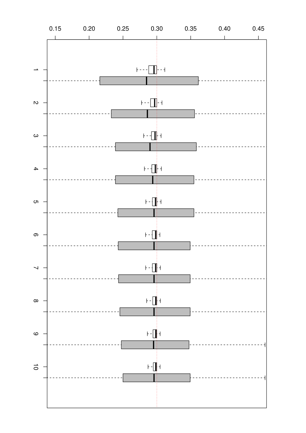
We expect the speed of convergence for estimating 𝐩\mathbf{p} is much slower than the one for estimating 𝐚\mathbf{a}. This is supported by our simulation experiment provided in Section 6 but we leave this question for further research. Section 3 is devoted to the proof of the consistency of 𝐚n¯\overline{\mathbf{a}_{n}} and 𝐚^n\widehat{\mathbf{a}}_{n} whereas Section 4 is devoted to the proof of the consistency of 𝐩^n\widehat{\mathbf{p}}_{n} and 𝐩n¯\overline{\mathbf{p}_{n}}.

Concluding remarks. Let us start to describe a naive estimation based on recurrence. For all xx in ℛn\mathcal{R}_{n}, we can estimate the environment at this point by

ω^x(n)=ξ+​(n,x)ξ⁡(n−1,x).\hat{\omega}_{x}^{(n)}=\frac{\xi^{+}(n,x)}{\xi(n-1,x)}.

By recurrence, ω^x(n)\hat{\omega}_{x}^{(n)} converges to ωx\omega_{x}, 𝐏⋆\mathbf{P}^{\star}-a.s. With some extra work, it can be shown that,

1Rn​∑x∈ℛnδω^x(n)→n→∞ηθ⋆𝐏⋆-a.s.,\frac{1}{R_{n}}\sum_{x\in\mathcal{R}_{n}}\delta_{\hat{\omega}_{x}^{(n)}}\xrightarrow[n\rightarrow\infty]{}\eta_{\theta^{\star}}\quad\mbox{$\mathbf{P}^{\star}$-a.s.},

where ℛn\mathcal{R}_{n} is defined by (9), and this leads to estimators of the parameters. This empirical estimator is then consistent. However, it gives equal weight to all visited sites xx in ℛn{\mathcal{R}}_{n}, without any notice of the number of visits there, which is certainly far from optimal. This is essentially how Adelman and Enriquez (2004) devise their estimators, and the simulations in Section 6 indicate they perform poorly at some extend. On the other hand, Andreoletti (2011) proposes estimators based on local time of the walk, which indeed take care of this flaw, but which are adhoc in essence and difficult to use in an optimal manner. In contrast, our estimate relies on first principles - maximum likelihood - and uses the full information gathered by the walk all through.

3 Proof of consistency for the MLE and MPLE of the ordered support

In the present section, we first recall the weak convergence result established by Gantert et al. for the empirical distributions of the RWRE. Then, we identify the limit of our criterion as a functional of 𝐚\mathbf{a} only, and provide some information on it. Using its regularity properties, we can adapt the proof of consistency for M-estimators to our context.

3.1 Potential and infinite valley

The environment ω\omega in which the random walk evolves is visualized as a potential landscape VV where V={V⁡(x):x∈ℤ}V=\{V(x)\,:\,x\in\mathbb{Z}\} is defined by

V⁡(x)={∑y=1xlog⁡ρyif x>0,0if x=0,−∑y=x+10logρyif x<0,V(x)=\left\{\begin{array}[]{ll}\sum_{y=1}^{x}\log\rho_{y}&\mbox{if $x>0$,}\\ 0&\mbox{if $x=0$,}\\ -\sum_{y=x+1}^{0}\log\rho_{y}&\mbox{if $x<0$,}\end{array}\right. (26)

with ρy=(1−ωy)/ωy\rho_{y}=(1-\omega_{y})/\omega_{y}. An example of a realization of VV can be seen on Figure 1.

Setting C⁡(x,x+1)=exp⁡[−V⁡(x)]C(x,x+1)=\exp[-V(x)], for any integer xx, the Markov chain XX is an electric network in the sense of Doyle and Snell (1984) or Levin et al. (2009), where C⁡(x,x+1)C(x,x+1) is the conductance of the (unoriented) bond (x,x+1)(x,x+1). In particular, the measure μ\mu defined as

μ⁡(x)=exp⁡[−V⁡(x−1)]+exp⁡[−V⁡(x)],x∈ℤ,\mu(x)=\exp[-V(x-1)]+\exp[-V(x)],\quad x\in\mathbb{Z}, (27)

is a reversible and invariant measure for the Markov chain XX.

Now, define the right border cnc_{n} of the “valley” with depth log⁡n+(log⁡n)1/2\log n+(\log n)^{1/2} as

cn=min⁡{x≥0:V⁡(x)−min0≤y≤x⁡V⁡(y)≥log⁡n+(log⁡n)1/2},c_{n}=\min\big\{x\geq 0\,:\,V(x)-\min_{0\leq y\leq x}V(y)\geq\log n+(\log n)^{1/2}\big\}, (28)

and the bottom bnb_{n} of the “valley” as

bn=min⁡{x≥0:V⁡(x)=min0≤y≤cn⁡V⁡(y)}.b_{n}=\min\big\{x\geq 0\,:\,V(x)=\min_{0\leq y\leq c_{n}}V(y)\big\}.

On Figure 1, one can see a representation of bnb_{n} and cnc_{n}. We are interested in the shape of the “valley” (0,bn,cn)(0,b_{n},c_{n}) when nn tends to infinity and we recall the concept of infinite valley introduced by Golosov (1984).

V⁡(x)V(x)xxbnb_{n}cnc_{n}log⁡n+log⁡n\log n+\sqrt{\log n}
Figure 1: Example of potential derived from a random environment distributed as in Example I with parameter a=0.3a=0.3. Simulation with n=1000n=1000.

Let V~={V~​(x):x∈ℤ}\widetilde{V}=\{\widetilde{V}(x)\,:\,x\in\mathbb{Z}\} be a collection of random variables distributed as VV conditioned to stay positive for any negative xx, and non-negative for any non negative xx. For simplicity, we assume that without loss of generality, V~\widetilde{V} is also realised under ℙ⋆\mathbb{P}^{\star}. For each realization of V~\widetilde{V}, consider the corresponding Markov chain on ℤ\mathbb{Z}, which is an electrical network with conductances C~​(x,x+1)=exp⁡[−V~​(x)]\widetilde{C}(x,x+1)=\exp[-\widetilde{V}(x)]. As usual, the measure μ~\widetilde{\mu} defined as μ~​(x)=C~​(x−1,x)+C~​(x,x+1)\widetilde{\mu}(x)=\widetilde{C}(x-1,x)+\widetilde{C}(x,x+1), x∈ℤx\in\mathbb{Z}, is a (reversible) and invariant measure for the Markov chain XX. Furthermore, the measure μ~\widetilde{\mu} can be normalized to get a reversible probability measure ν\nu, defined by

ν⁡(x)=exp⁡[−V~​(x−1)]+exp⁡[−V~​(x)]2​∑z∈ℤexp⁡[−V~​(z)].\nu(x)=\frac{\exp[-\widetilde{V}(x-1)]+\exp[-\widetilde{V}(x)]}{2\sum_{z\in\mathbb{Z}}\exp[-\widetilde{V}(z)]}. (29)

Note that ν⁡(x)\nu(x) can be written as the sum of ν+​(x)\nu^{+}(x) and ν−​(x)\nu^{-}(x), where for any x∈ℤx\in\mathbb{Z}

ν+​(x)=exp⁡[−V~​(x)]2​∑z∈ℤexp⁡[−V~​(z)]andν−​(x)=exp⁡[−V~​(x−1)]2​∑z∈ℤexp⁡[−V~​(z)].\nu^{+}(x)=\frac{\exp[-\widetilde{V}(x)]}{2\sum_{z\in\mathbb{Z}}\exp[-\widetilde{V}(z)]}\quad\mbox{and}\quad\nu^{-}(x)=\frac{\exp[-\widetilde{V}(x-1)]}{2\sum_{z\in\mathbb{Z}}\exp[-\widetilde{V}(z)]}. (30)

We have ν+​(x)=ν−​(x+1)\nu^{+}(x)=\nu^{-}(x+1). Define ω~​(x)∈(0,1)\widetilde{\omega}(x)\in(0,1), for any x∈ℤx\in\mathbb{Z}, as

ω~​(x)=ν+​(x)ν⁡(x)=11+exp⁡[V~​(x)−V~​(x−1)].\widetilde{\omega}(x)=\frac{\nu^{+}(x)}{\nu(x)}=\frac{1}{1+\exp[\widetilde{V}(x)-\widetilde{V}(x-1)]}. (31)
Remark 3.1.

Noting that the possible values of V~​(x)−V~​(x−1)\widetilde{V}(x)-\tilde{V}(x-1) are those of V⁡(x)−V⁡(x−1)V(x)-V(x-1) for any integer xx, we deduce that under ℙ⋆\mathbb{P}^{\star}, ω~​(x)\widetilde{\omega}(x) is equal to one of the coordinates of 𝐚⋆\mathbf{a}^{\star}.

Gantert et al. (2010) showed that the empirical distribution of the RWRE, suitably centered at bnb_{n} converges to the stationary distribution of a random walk in an infinite valley. More precisely, let

νn(x)=ν(n,x+bn),νn+(x)=ν+(n,x+bn),andνn−(x)=ν−(n,x+bn).\nu_{n}(x)=\nu(n,x+b_{n}),\quad\nu^{+}_{n}(x)=\nu^{+}(n,x+b_{n}),\quad\mbox{and}\quad\nu^{-}_{n}(x)=\nu^{-}(n,x+b_{n}).
Theorem 3.2 (Gantert et al. (2010)).

Let Assumptions I and II hold. The distributions of {νn​(x):x∈ℤ}\{\nu_{n}(x)\,:\,x\in\mathbb{Z}\} converge weakly to the distribution of ν\nu (as probability measures on ℓ1\ell^{1} equipped with the ℓ1\ell_{1}-norm). As a consequence, for each strongly continuous functional f:ℓ1→ℝf:\ell^{1}\rightarrow\mathbb{R} which is shift invariant, we have

f⁡({ν⁡(n,x):x∈ℤ})→n→∞lawf⁡({ν⁡(x):x∈ℤ}).f\big(\{\nu(n,x)\,:\,x\in\mathbb{Z}\}\big)\xrightarrow[n\rightarrow\infty]{\mbox{{\small law}}}f\big(\{\nu(x)\,:\,x\in\mathbb{Z}\}\big).

In Gantert et al. (2010) is mentioned that the result still holds with obvious extensions for the non-reflected case, i.e., of a RWRE on ℤ\mathbb{Z}. An inspection of the proof of Gantert et al. immediatly yields:

Corollary 3.3.

Let Assumptions I and II hold. The distributions of

{(νn+​(x),νn−​(x)):x∈ℤ}\{(\nu^{+}_{n}(x),\nu^{-}_{n}(x))\,:\,x\in\mathbb{Z}\}

converge weakly to the distribution of {(ν+​(x),ν−​(x)):x∈ℤ}\{(\nu^{+}(x),\nu^{-}(x))\,:\,x\in\mathbb{Z}\}. As a consequence, for each strongly continuous functional f:ℓ1×ℓ1→ℝf:\ell^{1}\times\ell^{1}\rightarrow\mathbb{R} which is shift invariant, we have

f⁡({(ν+​(n,x),ν−​(n,x)):x∈ℤ})→n→∞lawf⁡({(ν+​(x),ν−​(x)):x∈ℤ}).f\big(\{(\nu^{+}(n,x),\nu^{-}(n,x))\,:\,x\in\mathbb{Z}\}\big)\xrightarrow[n\rightarrow\infty]{\mbox{{\small law}}}f\big(\{(\nu^{+}(x),\nu^{-}(x))\,:\,x\in\mathbb{Z}\}\big).

3.2 Identification and properties of the criterion limit

First, we start with

Proof of (22) in Lemma 2.2.

Clearly,

log⁡ε0×max0≤t≤n⁡Xt≤ℓn​(θ)−∑x∈ℛnmaxi≤d⁡{ξ+​(n,x)​log⁡ai+ξ−​(n,x)​log⁡(1−ai)}≤0,\log\varepsilon_{0}\times\max_{0\leq t\leq n}X_{t}\leq{\ell_{n}(\theta)}-\sum_{x\in\mathcal{R}_{n}}\max_{i\leq d}\Big\{\xi^{+}(n,x)\log a_{i}+\xi^{-}(n,x)\log(1-a_{i})\Big\}\leq 0, (32)

with ε0\varepsilon_{0} from (5), and from (12) and (13)

∑x∈ℛnmaxi≤d⁡{ξ+​(n,x)​log⁡ai+ξ−​(n,x)​log⁡(1−ai)}=n⋅Ln​(𝐚).\sum_{x\in\mathcal{R}_{n}}\max_{i\leq d}\Big\{\xi^{+}(n,x)\log a_{i}+\xi^{-}(n,x)\log(1-a_{i})\Big\}=n\cdot L_{n}(\mathbf{a}).

Since 𝐄⋆​(ρ0)≥exp⁡[𝐄⋆​log⁡(ρ0)]=1\mathbf{E}^{\star}(\rho_{0})\geq\exp[\mathbf{E}^{\star}\log(\rho_{0})]=1, case (c’) in Theorem 2.1.9 in Zeitouni (2004) applies, and Xn/nX_{n}/n converges to 0, 𝐏⋆\mathbf{P}^{\star}-a.s. Hence, 1n​max0≤t≤n​Xt\frac{1}{n}\max_{0\leq t\leq n}X_{t} converges to 0 𝐏⋆\mathbf{P}^{\star}-a.s and the claim is proved. ∎

For any 𝐚∈Θ𝐚\mathbf{a}\in\Theta_{\mathbf{a}}, denote L∞​(𝐚)L_{\infty}(\mathbf{a})

L∞​(𝐚)=L⁡(𝐚,ν+,ν−)=∑x∈ℤmaxi⁡{ν+​(x)​log⁡ai+ν−​(x)​log⁡(1−ai)},L_{\infty}(\mathbf{a})=L(\mathbf{a},\nu^{+},\nu^{-})=\sum_{x\in\mathbb{Z}}\max_{i}\big\{{\nu^{+}(x)}\log a_{i}+{\nu^{-}(x)}\log(1-a_{i})\big\}, (33)

where ν+\nu^{+} and ν−\nu^{-} are defined by (30). Anticipating Lemma 3.5 below, Corollary 3.3 and (22) immediatly yields

Ln​(𝐚)→n→∞lawL∞​(𝐚).L_{n}(\mathbf{a})\xrightarrow[n\rightarrow\infty]{\mbox{{\small law}}}L_{\infty}(\mathbf{a}).

Therefore, we provide some useful information on the functional L∞​(⋅)L_{\infty}(\cdot). To do so, some additional notations are required.

Definition 3.4 (Boltzmann entropy function and Kullback-Leibler distance).

Define the Boltzmann entropy function H⁡(⋅)H(\cdot) on (0,1)(0,1) as

H⁡(q)=−[q​log⁡q+(1−q)​log⁡(1−q)]≥0,H(q)=-[q\log q+(1-q)\log(1-q)]\geq 0,

the Kullback-Leibler distance dKL(⋅|⋅)d_{\mathrm{KL}}(\cdot|\cdot) on (0,1)×(0,1)(0,1)\times(0,1) as

dKL​(q|q′)=q​log⁡qq′+(1−q)​log⁡1−q1−q′≥0,d_{\mathrm{KL}}(q|q^{\prime})=q\log\frac{q}{q^{\prime}}+(1-q)\log\frac{1-q}{1-q^{\prime}}\geq 0,

and their multinomial extensions on probability vectors 𝐪\mathbf{q} and 𝐪′\mathbf{q}^{\prime}

H(𝐪)=−∑iqilogqi≥0,dKL(𝐪|𝐪′)=∑iqilogqiqi′≥0.H(\mathbf{q})=-\sum_{i}q_{i}\log q_{i}\geq 0,\quad d_{\mathrm{KL}}(\mathbf{q}|\mathbf{q}^{\prime})=\sum_{i}q_{i}\log\frac{q_{i}}{q^{\prime}_{i}}\geq 0.

With ν\nu and ω~\widetilde{\omega} defined by (29) and (31), we have for all 𝐚\mathbf{a} in Θa\Theta_{a} the identity

L∞(𝐚)=−∑x∈ℤν(x)H[ω~(x)]−∑x∈ℤν(x)mini(dKL[ω~(x)|ai]).L_{\infty}(\mathbf{a})=-\sum_{x\in\mathbb{Z}}\nu(x)H\big[\widetilde{\omega}(x)\big]-\sum_{x\in\mathbb{Z}}\nu(x)\min_{i}\big(d_{\mathrm{KL}}\big[\widetilde{\omega}(x)|a_{i}\big]\big). (34)

From Remark 3.1, we have mini⁡(dKL​[ω~​(x)|ai⋆])=0\min_{i}\big(d_{\mathrm{KL}}\big[\widetilde{\omega}(x)|a_{i}^{\star}\big]\big)=0, and using the fact that dKL​(q|q′)>0d_{\mathrm{KL}}(q|q^{\prime})>0 for q≠q′q\neq q^{\prime}, we deduce that

L∞(𝐚)<L∞(𝐚⋆)=−∑x∈ℤν(x)H[ω~(x)],𝐚≠𝐚⋆.L_{\infty}(\mathbf{a})<L_{\infty}(\mathbf{a}^{\star})=-\sum_{x\in\mathbb{Z}}\nu(x)H\big[\widetilde{\omega}(x)\big],\qquad\mathbf{a}\neq\mathbf{a}^{\star}. (35)

More precisely, a useful bound is

L∞​(𝐚)≤L∞​(𝐚⋆)−mink⁡(ν⁡{x∈ℤ:ω~​(x)=ak⋆})×∑j=1dmini⁡(dKL​[aj⋆|ai]),L_{\infty}(\mathbf{a})\leq L_{\infty}(\mathbf{a}^{\star})-\min_{k}\big(\nu\big\{x\in\mathbb{Z}\,:\,\widetilde{\omega}(x)=a^{\star}_{k}\big\}\big)\times\sum_{j=1}^{d}\min_{i}\big(d_{\mathrm{KL}}\big[a_{j}^{\star}|a_{i}\big]\big), (36)

where the sum is deterministic and positive for 𝐚≠𝐚⋆\mathbf{a}\neq\mathbf{a}^{\star}, though its factor (minj⁡(⋅)\min_{j}(\cdot)) is a.s. positive and does not depend on 𝐚\mathbf{a}.

Lemma 3.5.

The function LL defined by (12) is Lipschitz continuous:

|L⁡(𝐚,π+,π−)−L⁡(𝐚,μ+,μ−)|\displaystyle|L(\mathbf{a},\pi^{+},\pi^{-})-L(\mathbf{a},\mu^{+},\mu^{-})| ≤|log⁡ε0|⋅(‖π+−μ+‖1+‖π−−μ−‖1),\displaystyle\leq|\log\varepsilon_{0}|\cdot\big(\|\pi^{+}-\mu^{+}\|_{1}+\|\pi^{-}-\mu^{-}\|_{1}\big), (37)
|L⁡(𝐚,π+,π−)−L⁡(𝐚′,π+,π−)|\displaystyle|L(\mathbf{a},\pi^{+},\pi^{-})-L(\mathbf{a}^{\prime},\pi^{+},\pi^{-})| ≤2​ε0−1​‖𝐚−𝐚′‖2.\displaystyle\leq 2\varepsilon_{0}^{-1}\|\mathbf{a}-\mathbf{a}^{\prime}\|_{2}. (38)
Proof of Lemma 3.5.

Recall that ℝd∋u↦maxi⁡ui∈ℝ\mathbb{R}^{d}\ni u\mapsto\max_{i}u_{i}\in\mathbb{R} is 1-lipschitz continuous for the norm ∥⋅∥∞\|\cdot\|_{\infty}. Moreover, the mapping

fi:(𝐚,v+,v−)↦v+​log⁡ai+v−​log⁡(1−ai)f_{i}\,:\,(\mathbf{a},v^{+},v^{-})\mapsto v^{+}\log a_{i}+v^{-}\log(1-a_{i})

is |log⁡ε0||\log\varepsilon_{0}|-lipschitz continuous in v+v^{+}, resp. in v−v^{-}, with ε0\varepsilon_{0} from (5). By composition, (v+,v−)↦maxi⁡fi​(𝐚,v+,v−)(v^{+},v^{-})\mapsto\max_{i}f_{i}(\mathbf{a},v^{+},v^{-}) is |log⁡ε0||\log\varepsilon_{0}|-lipschitz continuous in the ∥⋅∥1\|\cdot\|_{1} norm, and (37) follows by summing over xx. By Cauchy-Schwarz,

|fi​(𝐚,v+,v−)−fi​(𝐚′,v+,v−)|\displaystyle|f_{i}(\mathbf{a},v^{+},v^{-})-f_{i}(\mathbf{a}^{\prime},v^{+},v^{-})| =|∫01∂afi​(𝐚′+t⁡(𝐚−𝐚′),v+,v−)⋅(𝐚−𝐚′)​𝑑t|\displaystyle=\Big|\int_{0}^{1}{\partial_{a}}f_{i}(\mathbf{a}^{\prime}+t(\mathbf{a}-\mathbf{a}^{\prime}),v^{+},v^{-})\cdot(\mathbf{a}-\mathbf{a}^{\prime})\mathrm{d}t\Big|
≤‖𝐚−𝐚′‖2×sup𝐚​"‖∂afi​(𝐚​",v+,v−)‖2,\displaystyle\leq\|\mathbf{a}-\mathbf{a}^{\prime}\|_{2}\times\sup_{\mathbf{a}"}\|{\partial_{a}}f_{i}(\mathbf{a}",v^{+},v^{-})\|_{2},

where derivative can be bounded using

‖∂afi​(𝐚,v+,v−)‖2=(ai−2​(v+)2+(1−ai)−2​(v−)2)1/2≤2​ε0−1​(v++v−).\|{\partial_{a}}f_{i}(\mathbf{a},v^{+},v^{-})\|_{2}=\left(a_{i}^{-2}(v^{+})^{2}+(1-a_{i})^{-2}(v^{-})^{2}\right)^{1/2}\leq 2\varepsilon_{0}^{-1}(v^{+}+v^{-}).

Taking the maximum over ii and summing over xx, this yields (38). ∎

3.3 Proof of Theorem 2.4

Recall that 𝐚n¯\overline{\mathbf{a}_{n}} is defined by (24). Fix some ε>0\varepsilon>0. We prove that for all ε1>0\varepsilon_{1}>0, there exists an integer n1n_{1} such that for all n≥n1n\geq n_{1},

𝐏⋆​(𝐚n¯∈ℬ⁡(𝐚⋆,ε))≥1−2​ε1,\mathbf{P}^{\star}\big(\overline{\mathbf{a}_{n}}\in{\mathcal{B}}(\mathbf{a}^{\star},\varepsilon)\big)\geq 1-2\varepsilon_{1}, (39)

where ℬ⁡(𝐚⋆,ε){\mathcal{B}}(\mathbf{a}^{\star},\varepsilon) is the open ball of radius ε\varepsilon centered at 𝐚⋆\mathbf{a}^{\star}.

Under ℙ⋆\mathbb{P}^{\star}, the sequence (g[ω~(x)]:x∈ℤ)(g[\widetilde{\omega}(x)]\,:\,x\in\mathbb{Z}) with g⁡(u)=log⁡(u−1−1)g(u)=\log(u^{-1}-1) is the sequence of the jumps of a random walk VV conditioned to stay positive. The jump of unconditionned VV takes the value g⁡(aj⋆)g(a_{j}^{\star}) with positive probability pj⋆p_{j}^{\star}. Hence it is not difficult to check that for all jj in {1,…,d}\{1,\dots,d\}, we can find ℙ⋆\mathbb{P}^{\star}-a.s. some random xx such that ω~​(x)=aj⋆\widetilde{\omega}(x)=a^{\star}_{j}. Since ν\nu is ℙ⋆\mathbb{P}^{\star}-a.s. supported by the whole ℤ\mathbb{Z}, we have

ℙ⋆​(minj⁡{ν⁡{x:ω~​(x)=aj⋆}}>0)=1.\mathbb{P}^{\star}\big(\min_{j}\big\{\nu\{x\,:\,\widetilde{\omega}(x)=a^{\star}_{j}\}\big\}>0\big)=1.

By continuity, for arbitrary ε1>0\varepsilon_{1}>0 we can fix δ1>0\delta_{1}>0 such that

ℙ⋆(minj{ν{x:ω~(x)=aj⋆}}≥δ1]≥1−ε1.\mathbb{P}^{\star}\Big(\min_{j}\big\{\nu\{x\,:\,\widetilde{\omega}(x)=a^{\star}_{j}\}\big\}\geq\delta_{1}\Big]\geq 1-\varepsilon_{1}. (40)

By compactness of K=Θ𝐚∖ℬ⁡(𝐚⋆,ε)K=\Theta_{\mathbf{a}}\setminus{\mathcal{B}}(\mathbf{a}^{\star},\varepsilon),

κ=inf{∑j=1dmini⁡{dKL​[aj⋆|ai]}:𝐚∈K}>0.\kappa=\inf\Big\{\sum_{j=1}^{d}\min_{i}\big\{d_{\mathrm{KL}}\big[a_{j}^{\star}|a_{i}\big]\big\}\,:\,\mathbf{a}\in K\Big\}>0.

By (38),

𝐚′∈ℬ⁡(𝐚,κ​δ1​ε0/6)⇒|L∞​(𝐚)−L∞​(𝐚′)|≤κ​δ1/3.\mathbf{a}^{\prime}\in{\mathcal{B}}\big(\mathbf{a},\kappa\delta_{1}\varepsilon_{0}/6\big)\Rightarrow|L_{\infty}(\mathbf{a})-L_{\infty}(\mathbf{a}^{\prime})|\leq\kappa\delta_{1}/3. (41)

Since KK is totally bounded, we can select a finite covering ∪k=1k0ℬ(𝐚k,κδ1ε0/6)\cup_{k=1}^{k_{0}}{\mathcal{B}}(\mathbf{a}^{k},\kappa\delta_{1}\varepsilon_{0}/6) of KK with balls of that radius. From (37) we can apply Corollary 3.3, and we have

(Ln(𝐚k): 0≤k≤k0)→n→∞law(L∞(𝐚k): 0≤k≤k0),\big(L_{n}(\mathbf{a}^{k})\,:\,0\leq k\leq k_{0}\big)\xrightarrow[n\rightarrow\infty]{\mbox{{\small law}}}\big(L_{\infty}(\mathbf{a}^{k})\,:\,0\leq k\leq k_{0}\big),

where we have set 𝐚0=𝐚⋆\mathbf{a}^{0}=\mathbf{a}^{\star}. Also,

(Ln​(𝐚⋆)−Ln​(𝐚k))k≤k0→n→∞law(L∞​(𝐚⋆)−L∞​(𝐚k))k≤k0,\big(L_{n}(\mathbf{a}^{\star})-L_{n}(\mathbf{a}^{k})\big)_{k\leq k_{0}}\xrightarrow[n\rightarrow\infty]{\mbox{{\small law}}}\big(L_{\infty}(\mathbf{a}^{\star})-L_{\infty}(\mathbf{a}^{k})\big)_{k\leq k_{0}},

where the limits are simultaneously larger than κ​δ1\kappa\delta_{1} on a set of large probability (larger than 1−ε11-\varepsilon_{1}) by (36) and (40). Then, we find n1n_{1} such that for n≥n1n\geq n_{1},

𝐏⋆(Ln(𝐚⋆)−Ln(𝐚k)≥2κδ1/3, 1≤k≤k0)≥1−2ε1.\mathbf{P}^{\star}\big(L_{n}(\mathbf{a}^{\star})-L_{n}(\mathbf{a}^{k})\geq 2\kappa\delta_{1}/3,\,1\leq k\leq k_{0}\big)\geq 1-2\varepsilon_{1}.

Taking (41) into account, we obtain that, for all n≥n1n\geq n_{1},

𝐏⋆(Ln(𝐚⋆)−Ln(𝐚)≥κδ1/3,𝐚∈K)≥1−2ε1.\mathbf{P}^{\star}\big(L_{n}(\mathbf{a}^{\star})-L_{n}(\mathbf{a})\geq\kappa\delta_{1}/3,\mathbf{a}\in K\big)\geq 1-2\varepsilon_{1}.

This implies (39) for all n≥n1n\geq n_{1}. Hence 𝐚n¯→𝐚⋆\overline{\mathbf{a}_{n}}\rightarrow\mathbf{a}^{\star} in 𝐏⋆\mathbf{P}^{\star}-probability. Now, we turn to the convergence of 𝐚^n\widehat{\mathbf{a}}_{n} to 𝐚⋆\mathbf{a}^{\star} in 𝐏⋆\mathbf{P}^{\star}-probability. According to (32), we have

Ln​(𝐚)−un≤ℓn​(θ)n≤Ln​(𝐚),L_{n}(\mathbf{a})-u_{n}\leq\frac{\ell_{n}(\theta)}{n}\leq L_{n}(\mathbf{a}),

where unu_{n} is non-negative and converges 𝐏⋆\mathbf{P}^{\star}-a.s. to 00 independently from θ\theta. Choosing n2n_{2} such that for all n≥n2n\geq n_{2}

𝐏⋆​(un≥κ​δ1/3)≤ε1,\mathbf{P}^{\star}\big(u_{n}\geq\kappa\delta_{1}/3\big)\leq\varepsilon_{1},

achieves the proof of the convergence 𝐚^n→𝐚⋆\widehat{\mathbf{a}}_{n}\rightarrow\mathbf{a}^{\star}.

4 Proof of consistency of estimates for the probability vector

First, note that Kn​(θ)K_{n}(\theta) can be rewritten

Kn​(θ)=−H⁡(Rn​(𝐚,⋅)Rn)−dKL​(Rn​(𝐚,⋅)Rn|𝐩).K_{n}(\theta)=-H\Big(\frac{R_{n}(\mathbf{a},\cdot)}{R_{n}}\Big)-d_{\mathrm{KL}}\Big(\frac{R_{n}(\mathbf{a},\cdot)}{R_{n}}\Big|\mathbf{p}\Big). (42)

Therefore,

Kn​(𝐚n¯,𝐩)\displaystyle K_{n}(\overline{\mathbf{a}_{n}},\mathbf{p}) ≤−H⁡(Rn​(𝐚n¯,⋅)Rn),\displaystyle\leq-H\Big(\frac{R_{n}(\overline{\mathbf{a}_{n}},\cdot)}{R_{n}}\Big),

with equality if and only if 𝐩=(Rn​(𝐚n¯,i)Rn:i=1,…,d)\mathbf{p}=\left(\frac{R_{n}(\overline{\mathbf{a}_{n}},i)}{R_{n}}\,:\,i=1,\ldots,d\right). Hence, we can use the alternative definition of 𝐩n¯\overline{\mathbf{p}_{n}} given by (25) to prove Theorem 2.5.

4.1 Proof of Theorem 2.5: convergence of 𝐩n¯\overline{\mathbf{p}_{n}}

For 0<δ<10<\delta<1 let

𝒢nδ\displaystyle\mathcal{G}_{n}^{\delta} ={x≤bn:maxz∈[x,bn]⁡V⁡(z)−V⁡(x)≥δ​log⁡n},\displaystyle=\big\{x\leq b_{n}\,:\,\max_{z\in[x,b_{n}]}V(z)-V(x)\geq\delta\log n\big\}, (43)
𝒟nδ\displaystyle\mathcal{D}_{n}^{\delta} ={x>bn:maxz∈[bn,x]⁡V⁡(z)−V⁡(bn)≤(1−δ)​log⁡n},\displaystyle=\big\{x>b_{n}\,:\,\max_{z\in[b_{n},x]}V(z)-V(b_{n})\leq(1-\delta)\log n\big\}, (44)
ℛnδ\displaystyle{\mathcal{R}}_{n}^{\delta} =𝒢nδ∪𝒟nδ.\displaystyle=\mathcal{G}_{n}^{\delta}\cup\mathcal{D}_{n}^{\delta}. (45)

Note that 𝒟nδ\mathcal{D}_{n}^{\delta} is an interval, 𝒟nδ=]bn,cnδ]\mathcal{D}_{n}^{\delta}=]b_{n},c_{n}^{\delta}] with cnδ≤cnc_{n}^{\delta}\leq c_{n}.

Denote 𝜷⋆\boldsymbol{\beta}^{\star} and 𝜷¯\overline{\boldsymbol{\beta}} the sequences defined by (14) replacing 𝐚\mathbf{a} by 𝐚⋆\mathbf{a}^{\star} and 𝐚n¯\overline{\mathbf{a}_{n}} respectively. Noting that for any ii in {1,…,d−1}\{1,\dots,d-1\}, dKL​(ai⋆|ai+1⋆)>0d_{\mathrm{KL}}(a_{i}^{\star}|a_{i+1}^{\star})>0, we can choose ε′>0\varepsilon^{\prime}>0 small enough such that for any i∈{1,…,d}i\in\{1,\ldots,d\}

βi−1⋆≤ai⋆1−ai⋆−2​ε′<ai⋆1−ai⋆+2​ε′≤βi⋆.\beta_{i-1}^{\star}\leq\frac{a^{\star}_{i}}{1-a_{i}^{\star}}-2\varepsilon^{\prime}<\frac{a^{\star}_{i}}{1-a_{i}^{\star}}+2\varepsilon^{\prime}\leq\beta_{i}^{\star}. (46)

Let ε>0\varepsilon>0. Define the events Anδ​(ε′)A_{n}^{\delta}(\varepsilon^{\prime}), Bn​(ε′)B_{n}(\varepsilon^{\prime}) and Cnδ​(ε,i)C_{n}^{\delta}(\varepsilon,i) by

Anδ​(ε′)\displaystyle A_{n}^{\delta}(\varepsilon^{\prime}) ={∀x∈ℛnδ:|ξ+(n,x)ξ−​(n,x)−1ρx|≤ε′},\displaystyle=\left\{\forall x\in{\mathcal{R}}_{n}^{\delta}\,:\,\Big|\frac{\xi+(n,x)}{\xi^{-}(n,x)}-\frac{1}{\rho_{x}}\Big|\leq\varepsilon^{\prime}\right\}, (47)
Bn​(ε′)\displaystyle B_{n}(\varepsilon^{\prime}) ={∀i∈{1,…,d}:|βi¯−βi⋆|≤ε′},\displaystyle=\left\{\forall i\in\{1,\ldots,d\}\,:\,|\overline{\beta_{i}}-\beta_{i}^{\star}|\leq\varepsilon^{\prime}\right\}, (48)
Cnδ​(ε,i)\displaystyle C_{n}^{\delta}(\varepsilon,i) ={|1|ℛn∩ℛnδ|∑x∈ℛn∩ℛnδ𝟙{ωx=ai⋆}−pi⋆|>ε4},\displaystyle=\left\{\Big|\frac{1}{|{\mathcal{R}}_{n}\cap{\mathcal{R}}_{n}^{\delta}|}\sum_{x\in{\mathcal{R}}_{n}\cap{\mathcal{R}}_{n}^{\delta}}\mathds{1}\{\omega_{x}=a_{i}^{\star}\}-p_{i}^{\star}\Big|>\frac{\varepsilon}{4}\right\}, (49)

Denote Aδn∁​(ε′){}^{\complement}A_{n}^{\delta}(\varepsilon^{\prime}) and Bn∁​(ε′){}^{\complement}B_{n}(\varepsilon^{\prime}) the respective complementary events of Anδ​(ε′)A_{n}^{\delta}(\varepsilon^{\prime}) and Bn​(ε′)B_{n}(\varepsilon^{\prime}), and define the quantities ϕnδ​(ε′)\phi_{n}^{\delta}(\varepsilon^{\prime}), ψnδ​(ε)\psi_{n}^{\delta}(\varepsilon) and μnδ​(ε)\mu_{n}^{\delta}(\varepsilon) by

ϕnδ​(ε′)\displaystyle\phi_{n}^{\delta}(\varepsilon^{\prime}) =𝐏⋆(∁Anδ(ε′))+𝐏⋆(∁Bn(ε′))\displaystyle=\mathbf{P}^{\star}\big(^{\complement}A_{n}^{\delta}(\varepsilon^{\prime})\big)+\mathbf{P}^{\star}\big(^{\complement}B_{n}(\varepsilon^{\prime})\big)
ψnδ​(ε)\displaystyle\psi_{n}^{\delta}(\varepsilon) =𝐏⋆​(|ℛn∖ℛnδ|Rn>ε2),\displaystyle=\mathbf{P}^{\star}\Big(\frac{|{\mathcal{R}}_{n}\setminus{\mathcal{R}}_{n}^{\delta}|}{R_{n}}>\frac{\varepsilon}{2}\Big),
μnδ​(ε,i)\displaystyle\mu_{n}^{\delta}(\varepsilon,i) =𝐏⋆​(Cnδ​(ε,i)).\displaystyle=\mathbf{P}^{\star}\Big(C_{n}^{\delta}(\varepsilon,i)\Big).

Then, we have

𝐏⋆​(|𝐩n¯​(i)−pi⋆|>ε)≤ϕnδ​(ε′)+ψnδ​(ε)+ψnδ​(ε/2)+μnδ​(ε,i).\mathbf{P}^{\star}\Big(\big|\overline{\mathbf{p}_{n}}(i)-p_{i}^{\star}\big|>\varepsilon\Big)\leq\phi_{n}^{\delta}(\varepsilon^{\prime})+\psi_{n}^{\delta}(\varepsilon)+\psi_{n}^{\delta}(\varepsilon/2)+\mu_{n}^{\delta}(\varepsilon,i). (50)

Indeed, it is clear that

𝐏⋆​(|𝐩n¯​(i)−pi⋆|>ε)≤𝐏⋆​(|𝐩n¯​(i)−pi⋆|>ε,Anδ​(ε′),Bn​(ε′))+ϕnδ​(ε′),\mathbf{P}^{\star}\Big(\big|\overline{\mathbf{p}_{n}}(i)-p_{i}^{\star}\big|>\varepsilon\Big)\leq\mathbf{P}^{\star}\Big(|\overline{\mathbf{p}_{n}}(i)-p_{i}^{\star}|>\varepsilon,A_{n}^{\delta}(\varepsilon^{\prime}),B_{n}(\varepsilon^{\prime})\Big)+\phi_{n}^{\delta}(\varepsilon^{\prime}), (51)

and writing the set ℛn{\mathcal{R}}_{n} as the union of the two disjoint sets (ℛn∩ℛnδ)\left({\mathcal{R}}_{n}\cap{\mathcal{R}}_{n}^{\delta}\right) and (ℛn∖ℛnδ)\left({\mathcal{R}}_{n}\setminus{\mathcal{R}}_{n}^{\delta}\right) in (18) and using (25) yields

𝐏⋆​(|𝐩n¯​(i)−pi⋆|>ε,Anδ​(ε′),Bn​(ε′))≤𝐏⋆​(Anδ​(ε′),Bn​(ε′),Dnδ​(ε,i))+ψnδ​(ε),\mathbf{P}^{\star}\Big(|\overline{\mathbf{p}_{n}}(i)-p_{i}^{\star}|>\varepsilon,A_{n}^{\delta}(\varepsilon^{\prime}),B_{n}(\varepsilon^{\prime})\Big)\leq\mathbf{P}^{\star}\Big(A_{n}^{\delta}(\varepsilon^{\prime}),B_{n}(\varepsilon^{\prime}),D_{n}^{\delta}(\varepsilon,i)\Big)+\psi_{n}^{\delta}(\varepsilon), (52)

with

Dnδ(ε,i)={|1Rn∑x∈ℛn∩ℛnδ𝟙{βi¯<ξ+​(n,x)ξ⁡(n,x)≤βi+1¯}−pi⋆|>ε2}.D_{n}^{\delta}(\varepsilon,i)=\left\{\Big|\frac{1}{R_{n}}\sum_{x\in{\mathcal{R}}_{n}\cap{\mathcal{R}}_{n}^{\delta}}\mathds{1}\Big\{\overline{\beta_{i}}<\frac{\xi^{+}(n,x)}{\xi(n,x)}\leq\overline{\beta_{i+1}}\Big\}-p_{i}^{\star}\Big|>\frac{\varepsilon}{2}\right\}.

Using our choice of ε′\varepsilon^{\prime} to satisfy (46), we have for all ii in {1,…,d}\{1,\dots,d\}

{βi¯<ξ+​(n,x)ξ⁡(n,x)≤βi+1¯,Anδ(ε′),Bn(ε′)}={ωx=ai⋆,Anδ(ε′),Bn(ε′)}.\left\{\overline{\beta_{i}}<\frac{\xi^{+}(n,x)}{\xi(n,x)}\leq\overline{\beta_{i+1}},A_{n}^{\delta}(\varepsilon^{\prime}),B_{n}(\varepsilon^{\prime})\right\}=\left\{\omega_{x}=a_{i}^{\star},A_{n}^{\delta}(\varepsilon^{\prime}),B_{n}(\varepsilon^{\prime})\right\}.

Hence,

𝐏⋆(Anδ(ε′),Bn(ε′),Dnδ(ε,i))≤𝐏⋆(|1Rn∑x∈ℛn∩ℛnδ𝟙{ωx=ai⋆}−pi⋆|>ε2),\mathbf{P}^{\star}\Big(A_{n}^{\delta}(\varepsilon^{\prime}),B_{n}(\varepsilon^{\prime}),D_{n}^{\delta}(\varepsilon,i)\Big)\leq\mathbf{P}^{\star}\Big(\Big|\frac{1}{R_{n}}\sum_{x\in{\mathcal{R}}_{n}\cap{\mathcal{R}}_{n}^{\delta}}\mathds{1}\{\omega_{x}=a_{i}^{\star}\}-p_{i}^{\star}\Big|>\frac{\varepsilon}{2}\Big), (53)

and clearly,

𝐏⋆(|1Rn∑x∈ℛn∩ℛnδ𝟙{ωx=ai⋆}−pi⋆|>ε2)≤ψnδ(ε/2)+μnδ(ε,i).\mathbf{P}^{\star}\Big(\Big|\frac{1}{R_{n}}\sum_{x\in{\mathcal{R}}_{n}\cap{\mathcal{R}}_{n}^{\delta}}\mathds{1}\{\omega_{x}=a_{i}^{\star}\}-p_{i}^{\star}\Big|>\frac{\varepsilon}{2}\Big)\leq\psi_{n}^{\delta}(\varepsilon/2)+\mu_{n}^{\delta}(\varepsilon,i). (54)

Combining (51), (52), (53) and (54) yields (50).

Anticipating some lemmas which are proved independently in the next section, we conclude the proof. From Lemma 4.1, we have

limδ→0lim supn→∞ψnδ​(ε)=0.\lim_{\delta\rightarrow 0}\ \limsup_{n\rightarrow\infty}\ \psi_{n}^{\delta}(\varepsilon)=0.

By the law of large numbers,

limn→∞μnδ​(ε)=0.\lim_{n\rightarrow\infty}\mu_{n}^{\delta}(\varepsilon)=0.

In view of (50), to conclude the proof of Theorem 2.5 it suffices to prove that, for all δ>0\delta>0, ϕnδ​(ε)\phi_{n}^{\delta}(\varepsilon) vanishes as n→∞n\rightarrow\infty. On the one hand, 𝐚n¯\overline{\mathbf{a}_{n}} converges to 𝐚⋆\mathbf{a}^{\star} in 𝐏⋆\mathbf{P}^{\star}-probability, and thus

𝐏⋆(∁Bn(ε′))⟶0.\mathbf{P}^{\star}\big(^{\complement}B_{n}(\varepsilon^{\prime})\big)\longrightarrow 0.

On the other hand, by Lemma 4.2,

𝐏⋆(∁Anδ(ε′))⟶0.\mathbf{P}^{\star}\big(^{\complement}A_{n}^{\delta}(\varepsilon^{\prime})\big)\longrightarrow 0.

This concludes the proof of the convergence in 𝐏⋆\mathbf{P}^{\star}-probability of 𝐩n¯\overline{\mathbf{p}_{n}} to 𝐩⋆\mathbf{p}^{\star}. □\Box

4.2 Proof of (23) in Lemma 2.2

For all x∈ℛnx\in\mathcal{R}_{n}, one can write

log⁡Ui​(𝐚,n,x)\displaystyle\log U_{i}(\mathbf{a},n,x) =[ξ+​(n,x)ξ⁡(n−1,x)−aı^​(𝐚,n,x)]​[log⁡aiaı^​(𝐚,n,x)−log⁡1−ai1−aı^​(𝐚,n,x)]\displaystyle=\Big[\frac{\xi^{+}(n,x)}{\xi(n-1,x)}-a_{{\hat{\imath}}(\mathbf{a},n,x)}\Big]\Big[\log\frac{a_{i}}{a_{{\hat{\imath}}(\mathbf{a},n,x)}}-\log\frac{1-a_{i}}{1-a_{{\hat{\imath}}(\mathbf{a},n,x)}}\Big] (55)
−dKL​(aı^​(𝐚,n,x)|ai).\displaystyle\qquad-d_{\mathrm{KL}}\big(a_{{\hat{\imath}}(\mathbf{a},n,x)}|a_{i}\big).

Let c0c_{0} be the quantity defined as

c0=inf𝐚∈Θ𝐚infi≠jdKL​(ai|aj)>0.c_{0}=\inf_{\mathbf{a}\in\Theta_{\mathbf{a}}}\inf_{i\neq j}d_{\mathrm{KL}}(a_{i}|a_{j})>0. (56)

where the strict inequality comes from (5) and the continuity of dKL(⋅|⋅)d_{\mathrm{KL}}(\cdot|\cdot). Recall ε0\varepsilon_{0} in (5) and ε′\varepsilon^{\prime} in (46), and let ε′′\varepsilon^{\prime\prime} be the quantity defined as

ε′′=min⁡{ε′,c04​(log⁡1−ε0ε0)−1}.\varepsilon^{\prime\prime}=\min\Big\{\varepsilon^{\prime},\frac{c_{0}}{4}\Big(\log\frac{1-\varepsilon_{0}}{\varepsilon_{0}}\Big)^{-1}\Big\}. (57)

Let 𝒱⁡(ε′′)⊂Θ𝐚\mathcal{V}(\varepsilon^{\prime\prime})\subset\Theta_{\mathbf{a}} be the neighborhood of 𝐚⋆\mathbf{a}^{\star} defined as

𝒱⁡(ε′′)={𝐚∈Θ𝐚:max⁡{‖𝐚−𝐚⋆‖,‖𝜷−𝜷⋆‖}≤ε′′}.\mathcal{V}(\varepsilon^{\prime\prime})=\Big\{\mathbf{a}\in\Theta_{\mathbf{a}}\,:\,\max\left\{\|\mathbf{a}-\mathbf{a}^{\star}\|,\|\boldsymbol{\beta}-\boldsymbol{\beta}^{\star}\|\right\}\leq\varepsilon^{\prime\prime}\Big\}. (58)

Fix 0<δ<10<\delta<1. Let 𝐚\mathbf{a} be in 𝒱⁡(ε′′)\mathcal{V}(\varepsilon^{\prime\prime}) and assume that Anδ​(ε′′)A_{n}^{\delta}(\varepsilon^{\prime\prime}) defined by (47) occurs, then for all x∈ℛnδx\in{\mathcal{R}}_{n}^{\delta} and any i≠ı^​(𝐚,n,x)i\neq{\hat{\imath}}(\mathbf{a},n,x)

log⁡Ui​(𝐚,n,x)≤−c02.\log U_{i}(\mathbf{a},n,x)\leq-\frac{c_{0}}{2}. (59)

Indeed, using (58) and the fact that Anδ​(ε′′)A_{n}^{\delta}(\varepsilon^{\prime\prime}) occurs with ε′′≤ε′\varepsilon^{\prime\prime}\leq\varepsilon^{\prime}, we have for all x∈ℛnδx\in\mathcal{R}_{n}^{\delta}

ı^​(𝐚,n,x)=ı^​(𝐚⋆,n,x)andωx=aı^​(𝐚,n,x)⋆=aı^​(𝐚⋆,n,x)⋆.{\hat{\imath}}(\mathbf{a},n,x)={\hat{\imath}}(\mathbf{a}^{\star},n,x)\quad\mbox{and}\quad\omega_{x}=a_{{\hat{\imath}}(\mathbf{a},n,x)}^{\star}=a_{{\hat{\imath}}(\mathbf{a}^{\star},n,x)}^{\star}. (60)

Then, if i≠ı^​(𝐚,n,x)i\neq{\hat{\imath}}(\mathbf{a},n,x), using (55), (56), (60), and the fact that

|log⁡aiaı^​(𝐚,n,x)−log⁡1−ai1−aı^​(𝐚,n,x)|≤2​log⁡1−ε0ε0,\Big|\log\frac{a_{i}}{a_{{\hat{\imath}}(\mathbf{a},n,x)}}-\log\frac{1-a_{i}}{1-a_{{\hat{\imath}}(\mathbf{a},n,x)}}\Big|\leq 2\log\frac{1-\varepsilon_{0}}{\varepsilon_{0}},

yield

log⁡Ui​(𝐚,n,x)≤2​log⁡1−ε0ε0​(|h⁡(ξ+​(n,x)ξ−​(n,x))−h⁡(1ρx)|+‖𝐚−𝐚⋆‖)−c0\log U_{i}(\mathbf{a},n,x)\leq 2\log\frac{1-\varepsilon_{0}}{\varepsilon_{0}}\left(\Big|h\big(\frac{\xi^{+}(n,x)}{\xi^{-}(n,x)}\big)-h\big(\frac{1}{\rho_{x}}\big)\Big|+\|\mathbf{a}-\mathbf{a}^{\star}\|\right)-c_{0}

with

h⁡(u)=u1+u.h(u)=\frac{u}{1+u}.

Using the fact that 0≤h′​(u)≤10\leq h^{\prime}(u)\leq 1, for any u≥0u\geq 0, and the fact that Anδ​(ε′′)A_{n}^{\delta}(\varepsilon^{\prime\prime}) occurs, we have

log⁡Ui​(𝐚,n,x)≤2​log⁡1−ε0ε0​(ε′′+‖𝐚−𝐚⋆‖)−c0.\log U_{i}(\mathbf{a},n,x)\leq 2\log\frac{1-\varepsilon_{0}}{\varepsilon_{0}}\left(\varepsilon^{\prime\prime}+\|\mathbf{a}-\mathbf{a}^{\star}\|\right)-c_{0}.

Using our choice of 𝐚\mathbf{a} and ε′′\varepsilon^{\prime\prime} achieves the proof of (59). Now, from (59), we deduce that if Anδ​(ε′′)A_{n}^{\delta}(\varepsilon^{\prime\prime}) occurs,

0≤rn(θ)≤|ℛn∖ℛnδ|⋅log(1+d−1ε0)+∑x∈ℛnδlog(1+d−1ε0e−ξ(n−1,x)c0/2).0\leq r_{n}(\theta)\leq\left|\mathcal{R}_{n}\setminus\mathcal{R}_{n}^{\delta}\right|\cdot\log\Big(1+\frac{d-1}{\varepsilon_{0}}\Big)+\sum_{x\in\mathcal{R}_{n}^{\delta}}\log\Big(1+\frac{d-1}{\varepsilon_{0}}\mathrm{e}^{-\xi(n-1,x)c_{0}/2}\Big). (61)

Assume that the event EnδE^{\delta}_{n} defined by

Enδ={∀x∈ℛnδ:ξ⁡(n,x)≥nδ/2},E^{\delta}_{n}=\left\{\forall x\in{\mathcal{R}}_{n}^{\delta}\,:\,\xi(n,x)\geq n^{\delta/2}\right\}, (62)

occurs. Then

0≤rn(θ)≤d−1ε0(|ℛn∖ℛnδ|+|ℛnδ|e−nδ/2c0/2).0\leq r_{n}(\theta)\leq\frac{d-1}{\varepsilon_{0}}\Big(\left|\mathcal{R}_{n}\setminus\mathcal{R}_{n}^{\delta}\right|+|\mathcal{R}_{n}^{\delta}|\mathrm{e}^{-n^{\delta/2}c_{0}/2}\Big). (63)

From Lemma 4.1, 4.2 and 4.3, we conclude that (23) occurs. □\Box

4.3 Convergence of 𝐩^n\widehat{\mathbf{p}}_{n}

From the definitions of θ^n\widehat{\theta}_{n} and 𝐚n¯\overline{\mathbf{a}_{n}} respectively given by (11) and (24), we have

ℓn​(θ^n)−ℓn​(θn¯)≥0andLn​(𝐚^n)−Ln​(𝐚n¯)≤0.\ell_{n}(\widehat{\theta}_{n})-\ell_{n}(\overline{\theta_{n}})\geq 0\quad\mbox{and}\quad L_{n}(\widehat{\mathbf{a}}_{n})-L_{n}(\overline{\mathbf{a}_{n}})\leq 0. (64)

Recalling (19), (64) implies

Kn​(θ^n)−Kn​(θn¯)+1Rn​[rn​(θ^n)−rn​(θn¯)]≥0.K_{n}(\widehat{\theta}_{n})-K_{n}(\overline{\theta_{n}})+\frac{1}{R_{n}}[r_{n}(\widehat{\theta}_{n})-r_{n}(\overline{\theta_{n}})]\geq 0. (65)

From Theorem 2.4, when nn is large enough, both 𝐚^n\widehat{\mathbf{a}}_{n} and 𝐚n¯\overline{\mathbf{a}_{n}} belong to 𝒱⁡(ε′′)\mathcal{V}(\varepsilon^{\prime\prime}) introduced in (58) with large probability. Assuming that the event Anδ​(ε′′)A_{n}^{\delta}(\varepsilon^{\prime\prime}) defined by (47) occurs, we have

ı^​(𝐚n¯,n,x)=ı^​(𝐚^n,n,x)=ı^​(𝐚⋆,n,x),for all x∈ℛnδ,{\hat{\imath}}(\overline{\mathbf{a}_{n}},n,x)={\hat{\imath}}(\widehat{\mathbf{a}}_{n},n,x)={\hat{\imath}}(\mathbf{a}^{\star},n,x),\quad\mbox{for all $x\in\mathcal{R}_{n}^{\delta}$},

and

Kn​(θ^n)≤log⁡(1−ε0ε0)​|ℛn∖ℛnδ|Rn+1Rn​∑x∈ℛnlog⁡p^ı^​(𝐚⋆,n,x),K_{n}(\widehat{\theta}_{n})\leq\log\Big(\frac{1-\varepsilon_{0}}{\varepsilon_{0}}\Big)\frac{|\mathcal{R}_{n}\setminus\mathcal{R}_{n}^{\delta}|}{R_{n}}+\frac{1}{R_{n}}\sum_{x\in\mathcal{R}_{n}}\log\widehat{p}_{{\hat{\imath}}(\mathbf{a}^{\star},n,x)},

as well as

Kn​(θn¯)≥log⁡(ε01−ε0)​|ℛn∖ℛnδ|Rn+1Rn​∑x∈ℛnlog⁡p¯ı^​(𝐚⋆,n,x),K_{n}(\overline{\theta_{n}})\geq\log\Big(\frac{\varepsilon_{0}}{1-\varepsilon_{0}}\Big)\frac{|\mathcal{R}_{n}\setminus\mathcal{R}_{n}^{\delta}|}{R_{n}}+\frac{1}{R_{n}}\sum_{x\in\mathcal{R}_{n}}\log\bar{p}_{{\hat{\imath}}(\mathbf{a}^{\star},n,x)},

which holds for large nn when 𝐩n¯\overline{\mathbf{p}_{n}} is in [ε0,1−ε0][\varepsilon_{0},1-\varepsilon_{0}], and finally

Kn​(θ^n)−Kn​(θn¯)≤2​log⁡(1−ε0ε0)​|ℛn∖ℛnδ|Rn−dKL​(𝐩n¯|𝐩^n).K_{n}(\widehat{\theta}_{n})-K_{n}(\overline{\theta_{n}})\leq 2\log\Big(\frac{1-\varepsilon_{0}}{\varepsilon_{0}}\Big)\frac{|\mathcal{R}_{n}\setminus\mathcal{R}_{n}^{\delta}|}{R_{n}}-d_{\mathrm{KL}}(\overline{\mathbf{p}_{n}}|\widehat{\mathbf{p}}_{n}). (66)

Assuming furthermore that EnδE_{n}^{\delta} defined by (62) occurs, then (63) occurs. All in all, combining (63), (65) and (66) yields the existence of a positive constant CC, depending on ε0\varepsilon_{0} and dd only, such that

dKL(𝐩n¯|𝐩^n)≤C(|ℛn∖ℛnδ|Rn+|ℛnδ|Rne−nδ/2c0/2),d_{\mathrm{KL}}(\overline{\mathbf{p}_{n}}|\widehat{\mathbf{p}}_{n})\leq C\Big(\frac{|\mathcal{R}_{n}\setminus\mathcal{R}_{n}^{\delta}|}{R_{n}}+\frac{|\mathcal{R}_{n}^{\delta}|}{R_{n}}\mathrm{e}^{-n^{\delta/2}c_{0}/2}\Big),

with large probability. From the fact that 𝐩n¯\overline{\mathbf{p}_{n}} converges in 𝐏⋆\mathbf{P}^{\star}-probability to 𝐩⋆\mathbf{p}^{\star}, the continuity of dKL(⋅|⋅)d_{\mathrm{KL}}(\cdot|\cdot), Lemma 4.1, 4.2 and 4.3, we conclude that 𝐩^n\widehat{\mathbf{p}}_{n} converges to 𝐩⋆\mathbf{p}^{\star} in 𝐏⋆\mathbf{P}^{\star}-probability. □\Box

4.4 Intermediate lemmas

Lemma 4.1.

There exists a random variable Z⁡(δ)≥0Z(\delta)\geq 0 such that

|ℛn∖ℛnδ|log2⁡n→n→∞lawZ⁡(δ),with\displaystyle\frac{\displaystyle\big|{\mathcal{R}}_{n}\setminus{\mathcal{R}}_{n}^{\delta}\big|}{\log^{2}n}\xrightarrow[n\rightarrow\infty]{\mbox{{\small law}}}Z(\delta),\quad\mbox{with} (67)
Z⁡(δ)→δ→00in 𝐏⋆-probability.\displaystyle Z(\delta)\xrightarrow[\delta\rightarrow 0]{}0\quad\mbox{in $\mathbf{P}^{\star}$-probability}. (68)
Proof.

By the invariance principle,

(V⁡([u​log2​n])log⁡n,u≥0)→n→∞law(W⁡(u),u≥0),\left(\frac{V([u\log^{2}n])}{\log n};u\geq 0\right)\xrightarrow[n\rightarrow\infty]{\mbox{{\small law}}}(W(u);u\geq 0), (69)

with WW a standard Brownian motion. Recall the definition of cnδc_{n}^{\delta}, 𝒟nδ=]bn,cnδ]\mathcal{D}_{n}^{\delta}=]b_{n},c_{n}^{\delta}] with 𝒟nδ\mathcal{D}_{n}^{\delta} from (44), and define

c∞=inf{u\displaystyle c_{\infty}=\inf\big\{u >0:W(u)−minv∈[0,u]W(v)≥1},b∞=Argminv∈[0,c∞]W(v),\displaystyle>0:W(u)-\min_{v\in[0,u]}W(v)\geq 1\big\},\qquad b_{\infty}=\mathop{\rm Argmin}_{v\in[0,c_{\infty}]}W(v),
c∞δ=min⁡{u>b∞:W⁡(u)−W⁡(b∞)≥1−δ}.\displaystyle c_{\infty}^{\delta}=\min\big\{u>b_{\infty}:W(u)-W(b_{\infty})\geq 1-\delta\big\}.

By (69) and from well-known results on RWRE (e.g., (Zeitouni, 2004, Sect. 2.5)), we have the joint convergence of

bnlog2⁡n→n→∞lawb∞,cnδlog2⁡n→n→∞lawc∞δ,max⁡ℛnlog2⁡n→n→∞lawc∞.\frac{b_{n}}{\log^{2}n}\xrightarrow[n\rightarrow\infty]{\mbox{{\small law}}}b_{\infty},\qquad\frac{c_{n}^{\delta}}{\log^{2}n}\xrightarrow[n\rightarrow\infty]{\mbox{{\small law}}}c_{\infty}^{\delta},\qquad\frac{\max{\mathcal{R}}_{n}}{\log^{2}n}\xrightarrow[n\rightarrow\infty]{\mbox{{\small law}}}c_{\infty}.

Then, the convergence in (67) follows, with the limit given by

Z⁡(δ)\displaystyle Z(\delta) =Leb⁡({u<b∞:maxv∈[u,b∞]⁡W⁡(v)−W⁡(u)≤δ}∪[c∞δ,c∞])\displaystyle={\rm Leb}\Big(\big\{u<b_{\infty}\,:\,\max_{v\in[u,b_{\infty}]}W(v)-W(u)\leq\delta\big\}\cup[c_{\infty}^{\delta},c_{\infty}]\Big)
=Z1​(δ)+Z2​(δ)\displaystyle=Z_{1}(\delta)+Z_{2}(\delta)

with Leb⁡(A){\rm Leb}(A) the Lebesgue measure of a Borel set AA and Z2​(δ)=c∞−c∞δZ_{2}(\delta)=c_{\infty}-c_{\infty}^{\delta}. It is not difficult to see that c∞δ↗c∞c_{\infty}^{\delta}\nearrow c_{\infty} a.s. as δ↘0\delta\searrow 0, and then Z2​(δ)Z_{2}(\delta) vanishes. Let us prove in details that Z1​(δ)Z_{1}(\delta) vanishes. Letting

Aδ={u<b∞:maxv∈[u,b∞]⁡W⁡(v)−W⁡(u)≤δ},A_{\delta}=\big\{u<b_{\infty}\,:\,\max_{v\in[u,b_{\infty}]}W(v)-W(u)\leq\delta\big\},

we have, as δ↘0\delta\searrow 0,

Aδ↘A0+⊂A′={u<b∞:W(u)≥W(v),v∈[u,b∞]}.A_{\delta}\searrow A_{0^{+}}\subset A^{\prime}=\big\{u<b_{\infty}\,:\,W(u)\geq W(v),v\in[u,b_{\infty}]\big\}.

By Fubini, we compute

𝐄⋆​Leb​(A′)\displaystyle\mathbf{E}^{\star}{\rm Leb}(A^{\prime}) =∫0∞𝐏⋆​(u<b∞,u∈A′)​𝑑u,\displaystyle=\int_{0}^{\infty}\mathbf{P}^{\star}(u<b_{\infty},u\in A^{\prime})du,

and we show that the integrand is zero. For all u≥0u\geq 0,

𝐏⋆​(u<b∞,u∈A′)\displaystyle\mathbf{P}^{\star}(u<b_{\infty},u\in A^{\prime}) =limα↘0𝐏⋆​(u<b∞,u∈A′,u≤b∞+α)\displaystyle=\lim_{\alpha\searrow 0}\mathbf{P}^{\star}(u<b_{\infty},u\in A^{\prime},u\leq b_{\infty}+\alpha)
≤lim supα↘0𝐏⋆​(W⁡(u)≥W⁡(v),v∈[u,u+α]),\displaystyle\leq\limsup_{\alpha\searrow 0}\mathbf{P}^{\star}(W(u)\geq W(v),v\in[u,u+\alpha]),

and the last probability is zero by Iterated Logarithm law (Karatzas and Shreve, 1991, Th. 9.12)). Finally, limδ→0Leb⁡(Aδ)=0\lim_{\delta\rightarrow 0}{\rm Leb}(A_{\delta})=0 a.s., ending the proof of (68). ∎

Lemma 4.2.

Let Assumptions I and II hold, let ε′\varepsilon^{\prime} and ε′′\varepsilon^{\prime\prime} be such that (46) and (57) are satisfied, and let Anδ​(ε′′)A^{\delta}_{n}(\varepsilon^{\prime\prime}) and Anδ​(ε′′)A^{\delta}_{n}(\varepsilon^{\prime\prime}) be the events defined by (47). Then the following convergence holds

𝐏⋆​(Anδ∁​(ε′)),𝐏⋆​(Anδ∁​(ε′′))→n→∞0,for any δ in (0,1).\mathbf{P}^{\star}\Big({}^{\complement}A^{\delta}_{n}(\varepsilon^{\prime})\Big),\ \mathbf{P}^{\star}\Big({}^{\complement}A^{\delta}_{n}(\varepsilon^{\prime\prime})\Big)\xrightarrow[n\rightarrow\infty]{}0,\quad\mbox{for any $\delta$ in $(0,1)$}. (70)
Proof.

Under Pω(⋅|ξ(n−1,x)=m)P_{\omega}(\cdot|\xi_{(}n-1,x)=m), the pair (ξ+​(n,x),ξ−​(n,x))(\xi^{+}(n,x),\xi^{-}(n,x)) is distributed as (B⁡(m,ωx),m−B⁡(m,ωx))({\mathrm{B}}(m,\omega_{x}),m-{\mathrm{B}}(m,\omega_{x})), where B⁡(m,q)\mathrm{B}(m,q) is a binomial random variable with sample size mm and probability of success qq. Using Hoeffding’s concentration inequality yields

Pω​(|ξ+​(n,x)m−ωx|>α|ξ⁡(n−1,x)=m)≤2​exp⁡[−2​m​α2],∀α>0.P_{\omega}\left(\Big|\frac{\xi^{+}(n,x)}{m}-\omega_{x}\Big|>\alpha\,\Big|\,\xi(n-1,x)=m\right)\leq 2\exp[-2m\alpha^{2}],\quad\forall\alpha>0. (71)

Assume that the event {ξ(n−1,x)=m}\{\xi(n-1,x)={m}\} occurs. Then, we have

|ξ+​(n,x)ξ−​(n,x)−1ρx|=|f⁡(ξ+​(n,x)m)−f⁡(ωx)|≤supIf′⋅|ξ+​(n,x)m−ωx|,\Big|\frac{\xi^{+}(n,x)}{\xi^{-}(n,x)}-\frac{1}{\rho_{x}}\Big|=\Big|f\Big(\frac{\xi^{+}(n,x)}{m}\Big)-f(\omega_{x})\Big|\leq\sup_{I}f^{\prime}\cdot\Big|\frac{\xi^{+}(n,x)}{m}-\omega_{x}\Big|,

with

f⁡(u)=u1−uandI=[ξ+​(n,x)m∧ωx,ξ+​(n,x)m∨ωx].f(u)=\frac{u}{1-u}\quad\mbox{and}\quad I=\left[\frac{\xi^{+}(n,x)}{m}\wedge\omega_{x},\frac{\xi^{+}(n,x)}{m}\vee\omega_{x}\right].

Under Assumption II, uniform ellipticity occurs and (71) implies that we can find a constant K>0K>0 depending on ε′′\varepsilon^{\prime\prime} only such that

Pω​(|ξ+​(n,x)ξ−​(n,x)−1ρx|>ε′′|ξ⁡(n−1,x)=m)≤K−1​exp⁡[−K​m].P_{\omega}\left(\Big|\frac{\xi^{+}(n,x)}{\xi^{-}(n,x)}-\frac{1}{\rho_{x}}\Big|>\varepsilon^{\prime\prime}\,\Big|\,\xi(n-1,x)=m\right)\leq K^{-1}\exp[-Km]. (72)

Recall the event EnδE^{\delta}_{n} defined by (62) and denote its complement by Enδ∁{}^{\complement}E^{\delta}_{n}. We have

Pω​(Anδ∁​(ε′′))≤Pω​(Anδ∁​(ε′′),Enδ)+Pω​(Enδ∁).P_{\omega}\left({}^{\complement}A^{\delta}_{n}(\varepsilon^{\prime\prime})\right)\leq P_{\omega}\left({}^{\complement}A^{\delta}_{n}(\varepsilon^{\prime\prime}),E^{\delta}_{n}\right)+P_{\omega}\left({}^{\complement}E^{\delta}_{n}\right).

Now,

Pω​(Anδ∁​(ε′′),Enδ)≤∑x∈ℛnδPω​(|ξ+​(n,x)ξ−​(n,x)−1ρx|>ε′′,ξ⁡(n−1,x)≥nδ/2),P_{\omega}\left({}^{\complement}A^{\delta}_{n}(\varepsilon^{\prime\prime}),E^{\delta}_{n}\right)\leq\sum_{x\in{\mathcal{R}}_{n}^{\delta}}P_{\omega}\left(\Big|\frac{\xi^{+}(n,x)}{\xi^{-}(n,x)}-\frac{1}{\rho_{x}}\Big|>\varepsilon^{\prime\prime},\xi(n-1,x)\geq n^{\delta/2}\right),

and writing {ξ(n−1,x)≥nδ/2}=⋃m≥nδ/2{ξ(n−1,x)=m}\left\{\xi(n-1,x)\geq n^{\delta/2}\right\}=\bigcup_{m\geq n^{\delta/2}}\{\xi(n-1,x)=m\} and using (72) yield

Pω​(Anδ∁​(ε′′),Enδ)≤∑x∈ℛnδ∑m≥nδ/2K−1​exp⁡[−K​m]⋅Pω​(ξ⁡(n−1,x)=m).P_{\omega}\left({}^{\complement}A^{\delta}_{n}(\varepsilon^{\prime\prime}),E^{\delta}_{n}\right)\leq\sum_{x\in{\mathcal{R}}_{n}^{\delta}}\sum_{m\geq n^{\delta/2}}K^{-1}\exp[-Km]\cdot P_{\omega}(\xi(n-1,x)=m).

Using the fact that

exp[−Km]≤exp[−Knδ/2],for any m≥nδ/2,\exp[-Km]\leq\exp[-Kn^{\delta/2}],\quad\mbox{for any $m\geq n^{\delta/2}$},

the fact that

∑m≥nδ/2Pω​(ξ⁡(n−1,x)=m)≤1,\sum_{m\geq n^{\delta/2}}P_{\omega}(\xi(n-1,x)=m)\leq 1,

and the fact that |ℛnδ|≤cn|{\mathcal{R}}_{n}^{\delta}|\leq c_{n}, yield

Pω​(Anδ∁​(ε′′),Enδ)≤K−1​cn​exp⁡[−K​nδ/2].P_{\omega}\left({}^{\complement}A^{\delta}_{n}(\varepsilon^{\prime\prime}),E^{\delta}_{n}\right)\leq K^{-1}c_{n}\exp[-Kn^{\delta/2}]. (73)

Then, combining (73) and

𝐏⋆​(Anδ∁​(ε′′),Enδ)=𝔼⋆​(Pω​(Anδ∁​(ε′′),Enδ))\mathbf{P}^{\star}\left({}^{\complement}A^{\delta}_{n}(\varepsilon^{\prime\prime}),E^{\delta}_{n}\right)=\mathbb{E}^{\star}\left(P_{\omega}\left({}^{\complement}A^{\delta}_{n}(\varepsilon^{\prime\prime}),E^{\delta}_{n}\right)\right)

yields

𝐏⋆​(Anδ∁​(ε′′),Enδ)≤K−1​exp⁡[−K​nδ/2]​log3​n+ℙ⋆​(cn>log3⁡n),\mathbf{P}^{\star}\left({}^{\complement}A^{\delta}_{n}(\varepsilon^{\prime\prime}),E^{\delta}_{n}\right)\leq K^{-1}\exp[-Kn^{\delta/2}]\log^{3}n+\mathbb{P}^{\star}(c_{n}>\log^{3}n),

and from the fact that cn/log2⁡nc_{n}/\log^{2}n converges in ℙ⋆\mathbb{P}^{\star}-distribution to c∞c_{\infty}, we deduce that

𝐏⋆(Anδ∁(ε′′),Enδ)→n→∞0,for any δ in (0,1).\mathbf{P}^{\star}\left({}^{\complement}A^{\delta}_{n}(\varepsilon^{\prime\prime}),E^{\delta}_{n}\right)\xrightarrow[n\rightarrow\infty]{}0,\quad\mbox{for any $\delta$ in $(0,1)$}.

From Lemma 4.3 below, we have

𝐏⋆​(Enδ∁)=𝔼⋆​(Pω​(Enδ∁))→n→∞0,for any δ in (0,1),\mathbf{P}^{\star}\left({}^{\complement}E^{\delta}_{n}\right)=\mathbb{E}^{\star}\left(P_{\omega}\left({}^{\complement}E^{\delta}_{n}\right)\right)\xrightarrow[n\rightarrow\infty]{}0,\quad\mbox{for any $\delta$ in $(0,1)$},

and this achieves the proof of (70) since Anδ​(ε′′)⊂Anδ​(ε′)A^{\delta}_{n}(\varepsilon^{\prime\prime})\subset A^{\delta}_{n}(\varepsilon^{\prime}). ∎

Lemma 4.3.

Let Assumptions I and II hold and let EnδE^{\delta}_{n} be the event defined by (62). Then the following convergence holds

𝐏⋆​(Enδ∁)→n→∞0,for any δ in (0,1).\mathbf{P}^{\star}\left({}^{\complement}E^{\delta}_{n}\right)\xrightarrow[n\rightarrow\infty]{}0,\quad\mbox{for any $\delta$ in $(0,1)$}. (74)
Proof.

Note that

𝐏⋆(Enδ∁)≤𝐏⋆(∃x∈𝒢nδ:ξ(n,x)<nδ/2)+𝐏⋆(∃x∈𝒟nδ:ξ(n,x)<nδ/2),\mathbf{P}^{\star}\left({}^{\complement}E^{\delta}_{n}\right)\leq\mathbf{P}^{\star}\left(\exists x\in\mathcal{G}_{n}^{\delta}\,:\,\xi(n,x)<n^{\delta/2}\right)+\mathbf{P}^{\star}\left(\exists x\in\mathcal{D}_{n}^{\delta}\,:\,\xi(n,x)<n^{\delta/2}\right),

where 𝒢nδ\mathcal{G}_{n}^{\delta} and 𝒟nδ\mathcal{D}_{n}^{\delta} are respectively defined by (43) and (44). We first show that

𝐏⋆(∃x∈𝒟nδ:ξ(n,x)<nδ/2)→n→∞0,for any δ in (0,1).\mathbf{P}^{\star}\left(\exists x\in\mathcal{D}_{n}^{\delta}\,:\,\xi(n,x)<n^{\delta/2}\right)\xrightarrow[n\rightarrow\infty]{}0,\quad\mbox{for any $\delta$ in $(0,1)$}. (75)

Let xx be in 𝒟nδ\mathcal{D}_{n}^{\delta}. Define T⁡(y)=inf{t≥1:Xt=y}T(y)=\inf\{t\geq 1\,:\,X_{t}=y\} the first hitting time of yy. The probability of visiting x>bnx>b_{n} during a given excursion from bnb_{n} to bnb_{n} is (e.g., (Zeitouni, 2004, formula (2.1.4)))

Pω​(T⁡(x)<T⁡(bn)|X0=bn)=ωbn∑j=bnxexp⁡[V⁡(j)−V⁡(bn)]>ε0cn⋅nδ−1,P_{\omega}(T(x)<T(b_{n})\,|\,X_{0}=b_{n})=\frac{\omega_{b_{n}}}{\sum_{j=b_{n}}^{x}\exp[V(j)-V(b_{n})]}>\frac{\varepsilon_{0}}{c_{n}}\cdot n^{\delta-1}, (76)

where the lower bound follows from (4) and the fact that xx belongs to 𝒟nδ\mathcal{D}_{n}^{\delta}.

Fix ε>0\varepsilon>0 and let knk_{n} denote the number of excursions of XX from bnb_{n} to bnb_{n} before time nn. From (2.14) in Gantert et al. (2010), we have

Pω​(|knn−1γn|≥ε)→n→∞0,for ℙ⋆-a.a. ω,P_{\omega}\Big(\Big|\frac{k_{n}}{n}-\frac{1}{\gamma_{n}}\Big|\geq\varepsilon\Big)\xrightarrow[n\rightarrow\infty]{}0,\quad\mbox{for \quad$\mathbb{P}^{\star}$-a.a. $\omega$},

where γn\gamma_{n} is the average length of an excursion from bnb_{n} to bnb_{n}. Let FnF_{n} denote the event Fn={kn≥n⋅γn−1/2}F_{n}=\left\{k_{n}\geq n\cdot\gamma_{n}^{-1}/2\right\}. We have

Pω(∃x∈𝒟nδ:ξ(n,x)<nδ/2,Fn)≤∑x∈𝒟nδPω(ξ(n,x)<nδ/2,Fn).P_{\omega}\left(\exists x\in\mathcal{D}_{n}^{\delta}\,:\,\xi(n,x)<n^{\delta/2},\,F_{n}\right)\leq\sum_{x\in\mathcal{D}_{n}^{\delta}}P_{\omega}\left(\xi(n,x)<n^{\delta/2},\,F_{n}\right).

Using the independence of excursions from bnb_{n} to bnb_{n} yields

Pω​(ξ⁡(n,x)<nδ/2,Fn)≤Prob⁡(B⁡(n⋅γn−1/2,ε0​cn−1​nδ−1)≤nδ/2),P_{\omega}\left(\xi(n,x)<n^{\delta/2},\,F_{n}\right)\leq\mathrm{Prob}\big(\mathrm{B}\left(n\cdot\gamma_{n}^{-1}/2,\varepsilon_{0}c_{n}^{-1}n^{\delta-1}\right)\leq n^{\delta/2}\big),

where B⁡(m,q)\mathrm{B}(m,q) is a binomial random variable with sample size mm and probability of success qq. Combining the Chernov’s bound

Prob⁡(B⁡(m,q)≤m⁡(q−α))≤exp⁡[−m​dKL​(q−α|q)].\mathrm{Prob}\big(\mathrm{B}(m,q)\leq m(q-\alpha)\big)\leq\exp\big[-md_{\mathrm{KL}}(q-\alpha|q)\big].

with m=n⋅γn−1/2m=n\cdot\gamma_{n}^{-1}/2, q=ε0​cn−1​nδ−1q=\varepsilon_{0}c_{n}^{-1}n^{\delta-1} and m⁡(q−α)=nδ/2m(q-\alpha)=n^{\delta/2}, the fact that |𝒟nδ|≤cn|\mathcal{D}_{n}^{\delta}|\leq c_{n}, that

γn=∑x=0cnμ⁡(x)μ⁡(bn)≤2​(1+cn),\gamma_{n}=\sum_{x=0}^{c_{n}}\frac{\mu(x)}{\mu(b_{n})}\leq 2(1+c_{n}),

and that

cnlog2⁡n→n→∞lawc∞,\frac{c_{n}}{\log^{2}n}\xrightarrow[n\rightarrow\infty]{\mbox{{\small law}}}c_{\infty},

yield (75).

Now, we turn to the case where xx is in 𝒢nδ\mathcal{G}_{n}^{\delta}, and a different argument is needed. From Lemma 1 in Golosov (1984),

𝐏⋆​(T⁡(bn)>n)→n→∞0,\mathbf{P}^{\star}(T(b_{n})>n)\xrightarrow[n\rightarrow\infty]{}0,

hence,

𝐏⋆​(ξ⁡(n,bn)=0)→n→∞0.\mathbf{P}^{\star}(\xi(n,b_{n})=0)\xrightarrow[n\rightarrow\infty]{}0.

Note that

{∃x∈𝒢nδ:ξ(n,x)=0}⊂{ξ(n,bn)=0}.\big\{\exists x\in\mathcal{G}_{n}^{\delta}\,:\,\xi(n,x)=0\big\}\subset\big\{\xi(n,b_{n})=0\big\}.

The probability of visiting bnb_{n} during a given excursion from xx to xx is

Pω​(T⁡(bn)<T⁡(x)|X0=x)=ωx∑j=xbnexp⁡[V⁡(j)−V⁡(x)]<n−δ,P_{\omega}(T(b_{n})<T(x)\,|\,X_{0}=x)=\frac{\omega_{x}}{\sum_{j=x}^{b_{n}}\exp[V(j)-V(x)]}<n^{-\delta}, (77)

where the larger bound follows the fact that xx belongs to 𝒢nδ\mathcal{G}_{n}^{\delta}. Let hn​(x)h_{n}(x) denote the number of returns to xx before reaching bnb_{n}. From (77), this is a geometric variable with success probability less than n−δn^{-\delta}. Now,

Pω(∃x∈𝒢nδ:ξ(n,x)≤nδ/2)≤Pω(∃x∈𝒢nδ: 1≤ξ(n,x)≤nδ/2)\displaystyle P_{\omega}\left(\exists x\in\mathcal{G}_{n}^{\delta}\,:\,\xi(n,x)\leq n^{\delta/2}\right)\leq P_{\omega}\left(\exists x\in\mathcal{G}_{n}^{\delta}\,:\,1\leq\xi(n,x)\leq n^{\delta/2}\right)
+Pω(∃x∈𝒢nδ:ξ(n,x)=0)\displaystyle+P_{\omega}\left(\exists x\in\mathcal{G}_{n}^{\delta}\,:\,\xi(n,x)=0\right)

Hence,

Pω(∃x∈𝒢nδ: 1≤ξ(n,x)≤nδ/2)\displaystyle P_{\omega}\left(\exists x\in\mathcal{G}_{n}^{\delta}\,:\,1\leq\xi(n,x)\leq n^{\delta/2}\right) ≤∑x∈𝒢nδPω​( 1≤ξ⁡(n,x)≤nδ/2)\displaystyle\leq\sum_{x\in\mathcal{G}_{n}^{\delta}}P_{\omega}\left(\,1\leq\xi(n,x)\leq n^{\delta/2}\right)
≤∑x∈𝒢nδPω​( 1≤hn​(x)≤nδ/2)\displaystyle\leq\sum_{x\in\mathcal{G}_{n}^{\delta}}P_{\omega}\left(\,1\leq h_{n}(x)\leq n^{\delta/2}\right)
≤|𝒢nδ|⋅[1−(1−n−δ)nδ/2]\displaystyle\leq|\mathcal{G}_{n}^{\delta}|\cdot[1-(1-n^{-\delta})^{n^{\delta/2}}]
≤cn⋅[1−(1−n−δ)nδ/2].\displaystyle\leq c_{n}\cdot[1-(1-n^{-\delta})^{n^{\delta/2}}].

Hence,

𝐏⋆(∃x∈𝒢nδ: 1≤ξ(n,x)≤nδ/2)≤[1−(1−n−δ)nδ/2]log3n+ℙ⋆(cn>log3n),\mathbf{P}^{\star}\left(\exists x\in\mathcal{G}_{n}^{\delta}\,:\,1\leq\xi(n,x)\leq n^{\delta/2}\right)\leq[1-(1-n^{-\delta})^{n^{\delta/2}}]\log^{3}n+\mathbb{P}^{\star}(c_{n}>\log^{3}n),

which combined with the fact that cn/log2⁡nc_{n}/\log^{2}n converges in distribution to c∞c_{\infty} proves that

𝐏⋆(∃x∈𝒢nδ:ξ(n,x)<nδ/2).∎\mathbf{P}^{\star}\left(\exists x\in\mathcal{G}_{n}^{\delta}\,:\,\xi(n,x)<n^{\delta/2}\right).\qed

5 Examples

5.1 Particular Case: recurrent Temkin model

Example I.

Let η=12​δa+12​δ1−a\eta=\frac{1}{2}\delta_{a}+\frac{1}{2}\delta_{1-a}. Here, the unknown parameter is the support a∈Θ⊂(0,1/2)a\in\Theta\subset(0,1/2) (namely θ=a\theta=a).

Proposition 5.1.

In the framework of Example I, the limiting function L∞L_{\infty} defined by (33) is deterministic and given by

L∞​(a)=−[H⁡(a⋆)+dKL​(a⋆|a)].L_{\infty}(a)=-\big[H(a^{\star})+d_{\mathrm{KL}}(a^{\star}|a)\big].
Proof.

Note that

{ω~(x),1−ω~(x)}={a⋆,1−a⋆},for any x∈ℤ.\{\widetilde{\omega}(x),1-\widetilde{\omega}(x)\}=\{a^{\star},1-a^{\star}\},\quad\mbox{for any $x\in\mathbb{Z}$}. (78)

Recalling that ν+​(x)=ν⁡(x)⋅ω~​(x)\nu^{+}(x)=\nu(x)\cdot\widetilde{\omega}(x) and ν−​(x)=ν⁡(x)⋅[1−ω~​(x)]\nu^{-}(x)=\nu(x)\cdot[1-\widetilde{\omega}(x)] and noting that

maxu∈{a,1−a}⁡{a⋆​log⁡u+(1−a⋆)​log⁡(1−u)}=a⋆​log⁡a+(1−a⋆)​log⁡(1−a),\max_{u\in\{a,1-a\}}\Big\{a^{\star}\log u+(1-a^{\star})\log(1-u)\Big\}=a^{\star}\log a+(1-a^{\star})\log(1-a),

implies that (33) might be rewritten as

L∞​(a)=[a⋆​log⁡a+(1−a⋆)​log⁡(1−a)]​∑xν⁡(x).L_{\infty}(a)=\Big[a^{\star}\log a+(1-a^{\star})\log(1-a)\Big]\sum_{x}\nu(x).

The fact that ∑x∈ℤν⁡(x)=1\sum_{x\in\mathbb{Z}}\nu(x)=1 achieves the proof. ∎

5.2 Case of two-point support

Example II.

Let η=p1​δa1+p2​δa2\eta=p_{1}\delta_{a_{1}}+p_{2}\delta_{a_{2}} with a1<1/2<a2a_{1}<1/2<a_{2}, and

p1=log⁡1−a1a1log⁡a2​(1−a1)a1​(1−a2),p2=log⁡a21−a2log⁡a2​(1−a1)a1​(1−a2).p_{1}=\frac{\log\frac{1-a_{1}}{a_{1}}}{\log\frac{a_{2}(1-a_{1})}{a_{1}(1-a_{2})}},\quad p_{2}=\frac{\log\frac{a_{2}}{1-a_{2}}}{\log\frac{a_{2}(1-a_{1})}{a_{1}(1-a_{2})}}.

Here, the unknown parameter is the support 𝐚=(a1,a2)\mathbf{a}=(a_{1},a_{2}).

The following result extends Proposition 5.1.

Proposition 5.2.

In the framework of Example II, the limiting function L∞L_{\infty} defined by (33) is deterministic and given by

L∞(𝐚)=−1a2⋆−a1⋆∑j=12|aj⋆−12|[H(aj⋆)+mini=1,2dKL(aj⋆|ai)].L_{\infty}(\mathbf{a})=-\frac{1}{a_{2}^{\star}-a_{1}^{\star}}\sum_{j=1}^{2}\Big|a_{j}^{\star}-\frac{1}{2}\Big|\big[H(a_{j}^{\star})+\min_{i=1,2}d_{\mathrm{KL}}(a_{j}^{\star}|a_{i})\big].
Proof.

By (34),

L∞(𝐚)=−∑j=12ν(j)⋅[H(aj⋆)+mini=1,2dKL(aj⋆|ai)],ν(j)=∑x:ω~​(x)=aj⋆ν(x).L_{\infty}(\mathbf{a})=-\sum_{j=1}^{2}\nu^{(j)}\cdot\big[H(a_{j}^{\star})+\min_{i=1,2}d_{\mathrm{KL}}(a_{j}^{\star}|a_{i})\big],\qquad\nu^{(j)}=\sum_{x:\widetilde{\omega}(x)=a^{\star}_{j}}\nu(x).

So, the formula for L∞​(𝐚)L_{\infty}(\mathbf{a}) follows from the values of the coefficients ν(j)\nu^{(j)}: these are determined by

∑j=12ν(j)=1,∑j=12ν(j)⋅(2​aj⋆−1)=0,\sum_{j=1}^{2}\nu^{(j)}=1,\qquad\sum_{j=1}^{2}\nu^{(j)}\cdot(2a_{j}^{\star}-1)=0,

where the second equality means that the mean drift is zero in the recurrent case. Indeed, the drift per time unit on time interval [0,n][0,n], n−1​∑t=0n−1(2​ωXt−1)=∑xνn​(x)​(2​ω~​(x)−1)n^{-1}\sum_{t=0}^{n-1}(2\omega_{X_{t}}-1)=\sum_{x}\nu_{n}(x)(2\widetilde{\omega}(x)-1), vanishes as n→∞n\rightarrow\infty by the law of large numbers for martingales. For a direct derivation, we can write, from (30) and (31),

∑xν⁡(x)​ω~​(x)=∑xν+​(x)=∑xν−​(x)=∑xν⁡(x)​(1−ω~​(x)),\displaystyle\sum_{x}\nu(x)\widetilde{\omega}(x)=\sum_{x}\nu^{+}(x)=\sum_{x}\nu^{-}(x)=\sum_{x}\nu(x)(1-\widetilde{\omega}(x)),

and then ∑xν⁡(x)​(2​ω~​(x)−1)=0,\sum_{x}\nu(x)(2\widetilde{\omega}(x)-1)=0, which, after reorganizing the terms, gives the second equality above. ∎

5.3 Particular Case: recurrent lazy Temkin model

We present a simple example for which L∞​(⋅)L_{\infty}(\cdot) is a random variable.

Example III.

Let η=1−r2​δa+r​δ1/2+1−r2​δ1−a\eta=\frac{1-r}{2}\delta_{a}+r\delta_{1/2}+\frac{1-r}{2}\delta_{1-a} with a<1/2,r∈(0,1)a<1/2,r\in(0,1). Here, we have 𝐚=(a,12,1−a)\mathbf{a}=(a,\frac{1}{2},1-a) and 𝐩=(1−r2,r,1−r2)\mathbf{p}=(\frac{1-r}{2},r,\frac{1-r}{2}), and the unknown parameter is (a,r)(a,r).

Proposition 5.3.

In the framework of Example III, there exists a′∈(0,a⋆)a^{\prime}\in(0,a^{\star}), depending only on a⋆a^{\star}, such that the limiting function L∞​(𝐚)L_{\infty}(\mathbf{a}) is deterministic when a∈(0,a′]a\in(0,a^{\prime}] and random when a∈(a′,1/2)a\in(a^{\prime},1/2):

𝕍​ar⋆​(L∞​(𝐚))>0.{\mathbb{V}\mbox{ar}}^{\star}(L_{\infty}(\mathbf{a}))>0.
Proof.

Set 𝐚¯={a,1/2,1−a}{\underline{\mathbf{a}}}=\{a,1/2,1-a\}. By (34),

L∞​(𝐚)=\displaystyle L_{\infty}(\mathbf{a})= −ν(a⋆)⋅[H(a⋆)+min𝐚¯dKL(a⋆|⋅)]\displaystyle-\nu^{(a^{\star})}\cdot\big[H(a^{\star})+\min_{{\underline{\mathbf{a}}}}d_{\mathrm{KL}}(a^{\star}|\cdot)\big]
−ν(1−a⋆)⋅[H(1−a⋆)+min𝐚¯dKL(1−a⋆|⋅)]−ν(1/2)⋅H(1/2),\displaystyle\qquad-\nu^{(1-a^{\star})}\cdot\big[H(1-a^{\star})+\min_{{\underline{\mathbf{a}}}}d_{\mathrm{KL}}(1-a^{\star}|\cdot)\big]-\nu^{(1/2)}\cdot H(1/2),

with

ν(u)=∑x:ω~​(x)=uν(x),u∈𝐚¯.\nu^{(u)}=\sum_{x:\widetilde{\omega}(x)=u}\nu(x),\quad u\in{\underline{\mathbf{a}}}.

So, the formula for L∞​(𝐚)L_{\infty}(\mathbf{a}) follows from the values of the coefficients ν(u)\nu^{(u)}: these satisfy

∑u∈𝐚¯ν(u)=1,∑u∈𝐚¯ν(u)​(2​u−1)=0,\sum_{u\in{\underline{\mathbf{a}}}}\nu^{(u)}=1,\qquad\sum_{u\in{\underline{\mathbf{a}}}}\nu^{(u)}(2u-1)=0,

where the second equality is equivalent to ν(a⋆)=ν(1−a⋆)\nu^{(a^{\star})}=\nu^{(1-a^{\star})}. Hence, we have 2​ν(a⋆)+ν(1/2)=12\nu^{(a^{\star})}+\nu^{(1/2)}=1. Furthermore, noting that

H(a⋆)=H(1−a⋆)andmin𝐚¯dKL(a⋆|⋅)=min𝐚¯dKL(1−a⋆|⋅)H(a^{\star})=H(1-a^{\star})\quad\mbox{and}\quad\min_{{\underline{\mathbf{a}}}}d_{\mathrm{KL}}(a^{\star}|\cdot)=\min_{{\underline{\mathbf{a}}}}d_{\mathrm{KL}}(1-a^{\star}|\cdot)

yields

L∞(𝐚)=ν(1/2)[H(a⋆)+min𝐚¯dKL(a⋆|⋅)−H(1/2)]−[H(a⋆)+min𝐚¯dKL(a⋆|⋅)].L_{\infty}(\mathbf{a})=\nu^{(1/2)}\big[H(a^{\star})+\min_{{\underline{\mathbf{a}}}}d_{\mathrm{KL}}(a^{\star}|\cdot)-H(1/2)\big]-\big[H(a^{\star})+\min_{{\underline{\mathbf{a}}}}d_{\mathrm{KL}}(a^{\star}|\cdot)\big]. (79)

One can see that in (79), the quantities

[H(a⋆)+min𝐚¯dKL(a⋆|⋅)−H(1/2)]andmin𝐚¯dKL(a⋆|⋅)]\big[H(a^{\star})+\min_{{\underline{\mathbf{a}}}}d_{\mathrm{KL}}(a^{\star}|\cdot)-H(1/2)\big]\quad\mbox{and}\quad\min_{{\underline{\mathbf{a}}}}d_{\mathrm{KL}}(a^{\star}|\cdot)\big]

are deterministic. Hence, L∞​(𝐚)L_{\infty}(\mathbf{a}) is random if and only if ν(1/2)\nu^{(1/2)} is random and [H(a⋆)+min𝐚¯dKL(a⋆|⋅)−H(1/2)]\big[H(a^{\star})+\min_{{\underline{\mathbf{a}}}}d_{\mathrm{KL}}(a^{\star}|\cdot)-H(1/2)\big] is non zero.

The facts that dKL(a⋆|⋅)d_{\mathrm{KL}}(a^{\star}|\cdot) is continuous, decreasing on (0,a⋆)(0,a^{\star}), increasing on (a⋆,1)(a^{\star},1), null at a⋆a^{\star} and that

dKL​(a⋆|1/2)=H⁡(1/2)−H⁡(a⋆)anddKL​(a⋆|a)→a→0+∞,d_{\mathrm{KL}}(a^{\star}|1/2)=H(1/2)-H(a^{\star})\quad\mbox{and}\quad d_{\mathrm{KL}}(a^{\star}|a)\xrightarrow[a\rightarrow 0]{}+\infty,

yield the existence of a unique a′∈(0,a⋆)a^{\prime}\in(0,a^{\star}) such that

dKL​(a⋆|a′)=H⁡(1/2)−H⁡(a⋆),d_{\mathrm{KL}}(a^{\star}|a^{\prime})=H(1/2)-H(a^{\star}),

and as a consequence that for any a∈(0,a′]a\in(0,a^{\prime}],

min𝐚¯dKL(a⋆|⋅)=dKL(a⋆|a′)=H(1/2)−H(a⋆).\min_{{\underline{\mathbf{a}}}}d_{\mathrm{KL}}(a^{\star}|\cdot)=d_{\mathrm{KL}}(a^{\star}|a^{\prime})=H(1/2)-H(a^{\star}).

Hence, the limiting function L∞​(𝐚)L_{\infty}(\mathbf{a}) is deterministic and equal to −H⁡(1/2)=−log⁡2-H(1/2)=-\log 2, for any a∈(0,a′]a\in(0,a^{\prime}].

Now, let aa be in (a′,1/2)(a^{\prime},1/2). Recall that

ν(1/2)=∑x:ω~​(x)=1/2ν(x),withν(x)=exp⁡[−V~​(x−1)]+exp⁡[−V~​(x)]2​∑z∈ℤexp⁡[−V~​(z)],\nu^{(1/2)}=\sum_{x:\widetilde{\omega}(x)=1/2}\nu(x),\quad\mbox{with}\quad\nu(x)=\frac{\exp[-\widetilde{V}(x-1)]+\exp[-\widetilde{V}(x)]}{2\sum_{z\in\mathbb{Z}}\exp[-\widetilde{V}(z)]},

and that ω~​(x)=1/2\widetilde{\omega}(x)=1/2 if and only if V~​(x)=V~​(x−1)\widetilde{V}(x)=\widetilde{V}(x-1). Now, we focus on the potential of the infinite valley. Recall that V~​(0)=0,\widetilde{V}(0)=0, {V~​(x)}x≥0\{\widetilde{V}(x)\}_{x\geq 0} and {V~​(−x)}x≥0\{\widetilde{V}(-x)\}_{x\geq 0} are two independent Markov chains where V~​(x)\widetilde{V}(x) is non-negative for any non-negative xx and V~​(x)\widetilde{V}(x) is positive for any negative xx, see Golosov (1984). Especially, we have

ℙ⋆​(V~​(x+1)=0|V~​(x)=0)=1−ℙ⋆​(V~​(x+1)=log⁡ρ⋆|V~​(x)=0)=r,\mathbb{P}^{\star}\big(\widetilde{V}(x+1)=0\,|\,\widetilde{V}(x)=0\big)=1-\mathbb{P}^{\star}\big(\widetilde{V}(x+1)=\log\rho^{\star}\,|\,\widetilde{V}(x)=0\big)=r,

where we set ρ⋆=1−a⋆a⋆\rho^{\star}=\frac{1-a^{\star}}{a^{\star}}. Define the random variable T≥1T\geq 1 as T=inf{x∈ℕ:V~​(x)=log⁡ρ⋆}T=\inf\{x\in\mathbb{N}\,:\,\widetilde{V}(x)=\log\rho^{\star}\}. The random variable TT is distributed according to a geometric distribution with parameter of success 1−r1-r, and for any 0≤x≤T−10\leq x\leq T-1, the potential V~​(x)\widetilde{V}(x) is equal to 00. We have

ν(1/2)=∑x<0e−V~​(x)​𝟙V~​(x−1)=V~​(x)+(T−1)+∑x=T∞e−V~​(x)​𝟙V~​(x−1)=V~​(x)∑x≤0e−V~​(x)+(T−1)+∑x=T∞e−V~​(x)\nu^{(1/2)}=\frac{\sum_{x<0}\mathrm{e}^{-\widetilde{V}(x)}\mathds{1}_{\widetilde{V}(x-1)=\widetilde{V}(x)}+(T-1)+\sum_{x=T}^{\infty}\mathrm{e}^{-\widetilde{V}(x)}\mathds{1}_{\widetilde{V}(x-1)=\widetilde{V}(x)}}{\sum_{x\leq 0}\mathrm{e}^{-\widetilde{V}(x)}+(T-1)+\sum_{x=T}^{\infty}\mathrm{e}^{-\widetilde{V}(x)}}

Using the definition of (V~(x):x∈ℤ)(\widetilde{V}(x)\,:\,x\in\mathbb{Z}) and the strong Markov property, TT is independent of ℱ:=𝔖(V~(x):x≤0 or x≥T)\mathcal{F}:=\mathfrak{S}(\widetilde{V}(x)\,:\,x\leq 0\mbox{ or }x\geq T), hence

𝕍​ar⋆​[ν(1/2)|ℱ]=𝕍​ar⋆​(T−1+Υ′T−1+Υ),\mathbb{V}\mbox{ar}^{\star}[\nu^{(1/2)}|\mathcal{F}]=\mathbb{V}\mbox{ar}^{\star}\left(\frac{T-1+\Upsilon^{\prime}}{T-1+\Upsilon}\right),

with

Υ′=∑x<0;x≥Te−V~​(x)​𝟙V~​(x−1)=V~​(x)andΥ=∑x≤0;x≥Te−V~​(x).\Upsilon^{\prime}=\sum_{x<0;x\geq T}\mathrm{e}^{-\widetilde{V}(x)}\mathds{1}_{\widetilde{V}(x-1)=\widetilde{V}(x)}\quad\mbox{and}\quad\Upsilon=\sum_{x\leq 0;x\geq T}\mathrm{e}^{-\widetilde{V}(x)}.

Since Υ>Υ′,\Upsilon>\Upsilon^{\prime}, 𝕍​ar⋆​[ν(1/2)|ℱ]\mathbb{V}\mbox{ar}^{\star}[\nu^{(1/2)}|\mathcal{F}] is a non constant strictly positive random variable, hence

𝕍​ar⋆​(ν(1/2))=𝔼⋆​(𝕍​ar⋆​[ν(1/2)|ℱ])+𝕍​ar⋆​(𝔼⋆​[ν(1/2)|ℱ])>0.∎\mathbb{V}\mbox{ar}^{\star}(\nu^{(1/2)})=\mathbb{E}^{\star}\big(\mathbb{V}\mbox{ar}^{\star}[\nu^{(1/2)}|\mathcal{F}]\big)+\mathbb{V}\mbox{ar}^{\star}(\mathbb{E}^{\star}[\nu^{(1/2)}|\mathcal{F}])>0.\qed

6 Numerical performance

In this section, we explore the numerical performance of our estimation procedure in the frameworks of Examples I to III. We compare our performance with the performance of the estimator proposed by Adelman and Enriquez (2004) in the framework of Example I. An explicit description of the form of Adelman and Enriquez’s estimator in the particular case of the one-dimensional nearest neighbour path is provided in Section 5.1 of Comets et al. (2014). Therefore, one can estimate θ⋆{\theta^{\star}} by the solution of an appropriate system of equations, as illustrated below.

Example I (continued)

In this case the parameter θ\theta equals aa and we have

v\displaystyle v =𝔼⋆​[ω0]=12​a⋆+12​(1−a⋆)=12,\displaystyle=\mathbb{E}^{\star}[\omega_{0}]=\frac{1}{2}a^{\star}+\frac{1}{2}(1-a^{\star})=\frac{1}{2},
w\displaystyle w =𝔼⋆​[ω02]𝔼⋆​[ω0]={12​[a⋆]2+12​(1−a⋆)2}⋅v−1=[a⋆]2+(1−a⋆)2.\displaystyle=\frac{\mathbb{E}^{\star}[\omega_{0}^{2}]}{\mathbb{E}^{\star}[\omega_{0}]}=\{\frac{1}{2}[a^{\star}]^{2}+\frac{1}{2}(1-a^{\star})^{2}\}\cdot v^{-1}=[a^{\star}]^{2}+(1-a^{\star})^{2}.

Hence, among the visited sites, the proportion of those from which the first move is to the right (or to the left) gives no information on the parameter a⋆a^{\star}. We need to push to the sites visited at least twice to get some information. Among those from which the first move is to the right, the proportion of those from which the second move is also to the right gives an estimator for [a⋆]2+(1−a⋆)2[a^{\star}]^{2}+(1-a^{\star})^{2}. Using this observation, we can estimate a⋆a^{\star}.

We now present the three simulation experiments corresponding respectively to Examples I to III. The comparison with Adelman and Enriquez’s procedure is given only for Example I. For each of the three simulations, we a priori fix a parameter value θ⋆{\theta^{\star}} as given in Table 1 and repeat 1,000 times the procedure described below.

Simulation Estimated parameter
Example I a⋆=0.3a^{\star}=0.3
Example II (a1⋆,a2⋆)=(0.4,0.7)(a_{1}^{\star},a_{2}^{\star})=(0.4,0.7)
Example III (a⋆,r⋆)=(0.3,0.2)(a^{\star},r^{\star})=(0.3,0.2)
Table 1: Parameter values for each experiment.

We first generate a random environment according to ηθ⋆\eta_{\theta^{\star}} on the set of sites {1,…,105}\{1,\dots,10^{5}\}. In fact, we do not use the environment values for all the sites, since only few of these sites are visited by the walk. However the computation cost is very low comparing to the rest of the estimation procedure. Then, we run a random walk in this environment and stop it successively at nn, with n∈{104⋅k: 1≤k≤10}n\in\{10^{4}\cdot k\,:\,1\leq k\leq 10\}. For each stop, we estimate θ⋆{\theta^{\star}} according to our MPLE procedure (and Adelman and Enriquez’s one for the first simulation). In the cases of Examples I and III, the likelihood optimization procedure for the support a⋆a^{\star} was performed as a combination of golden section search and successive parabolic interpolation. In the case of Example II, the likelihood optimization procedure for (a1⋆,a2⋆)(a_{1}^{\star},a_{2}^{\star}) was performed according to the "L-BFGS-B" method of Byrd et al. (1995) which uses a limited-memory modification of the “BFGS” quasi-Newton method published simultaneously in 1970 by Broyden, Fletcher, Goldfarb and Shanno. In all three cases, the parameters in Table 1 are chosen such that the RWRE is recurrent.

Figure 2 shows the boxplots of our estimator and Adelman and Enriquez’s estimator obtained from 1,000 iterations of the procedures in Example I. First, we shall notify that in order to simplify the visualisation of the results, we removed in the boxplots corresponding to Example I about 13.5% of outliers values (outside 1.5 times the interquartile range above the upper quartile and below the lower quartile) from our estimator. Second, we shall also notify that about 16% of Adelman and Enriquez’s estimation procedures could not be achieved for the simple reason that the equation involving 𝐚⋆\mathbf{a}^{\star} had no solution. We observe that our procedure is far more accurate than Adelman and Enriquez’s, and that the accuracies of the procedure increase with the value of nn.

Figure 3 shows the boxplots of our estimator obtained from 1,000 iterations of the procedure in Example II. Once again, we shall notify that in order to simplify the visualisation of the results, we removed in the boxplots corresponding to Example II about 13% of outliers values from both estimators of a1⋆a_{1}^{\star} and a2⋆a_{2}^{\star}. We observe that the accuracy of the procedure is high, and that in this case, it does increase with the value of nn.

Figure 4 shows the boxplots of our estimator obtained from 1,000 iterations of the procedure in Example III. We shall notify that in order to simplify the visualisation of the results, we removed in the boxplots corresponding to Example III about 12.3% of outliers values from our estimator of a⋆a^{\star} and 2.8% of outliers values from our estimator of r⋆r^{\star}. We observe that the accuracy of the procedure is high for the parameter of the support and low for the probability parameter, even if in both cases, the accuracy increases with the value of nn.

Refer to caption
Figure 2: Boxplots of our estimator (left and white) and Adelman and Enriquez’s estimator (right and grey) obtained from 1,000 iterations and for values nn ranging in {104⋅k: 1≤k≤10}\{10^{4}\cdot k\,:\,1\leq k\leq 10\} (xx-axis indicates the value kk). The panel displays estimation of a⋆a^{\star} in Example I. The true value is indicated by an horizontal line.
Refer to caption
Refer to caption
Figure 3: Boxplots of our estimator obtained from 1,000 iterations in Example II and for values nn ranging in {104⋅k: 1≤k≤10}\{10^{4}\cdot k\,:\,1\leq k\leq 10\} (xx-axis indicates the value kk). Estimation of a1⋆a_{1}^{\star} (top panel) and a2⋆a_{2}^{\star} (bottom panel). The true values are indicated by horizontal lines.
Refer to caption
Refer to caption
Figure 4: Boxplots of our estimator obtained from 1,000 iterations in Example III and for values nn ranging in {104⋅k: 1≤k≤10}\{10^{4}\cdot k\,:\,1\leq k\leq 10\} (xx-axis indicates the value kk). Estimation of a⋆a^{\star} (top panel) and r⋆r^{\star} (bottom panel). The true values are indicated by horizontal lines.

Acknowledgments

The authors warmly thank Julien Chiquet for sharing many fruitful reflexions about programming syntax and parallel computing.

References

  • Adelman and Enriquez (2004) Adelman, O. and N. Enriquez (2004). Random walks in random environment: what a single trajectory tells. Israel J. Math. 142, 205–220.
  • Andreoletti (2011) Andreoletti, P. (2011). On the estimation of the potential of Sinai’s rwre. Braz. J. Probab. Stat. 25, 121–144.
  • Andreoletti and Diel (2012) Andreoletti, P. and R. Diel (2012). DNA unzipping via stopped birth and death processes with unknown transition probabilities. Applied Mathematics Research eXpress.
  • Baldazzi et al. (2007) Baldazzi, V., S. Bradde, S. Cocco, E. Marinari, and R. Monasson (2007). Inferring DNA sequences from mechanical unzipping data: the large-bandwidth case. Phys. Rev. E 75, 011904.
  • Baldazzi et al. (2006) Baldazzi, V., S. Cocco, E. Marinari, and R. Monasson (2006). Inference of DNA sequences from mechanical unzipping: an ideal-case study. Phys. Rev. Lett. 96, 128102.
  • Broyden (1970) Broyden, C. G. (1970). The convergence of a class of double-rank minimization algorithms. Journal of the Institute of Mathematics and Its Applications 6, 76–90.
  • Byrd et al. (1995) Byrd, R. H., P. Lu, J. Nocedal, and C. Y. Zhu (1995). A limited memory algorithm for bound constrained optimization. SIAM J. Sci. Comput. 16(5).
  • Chernov (1967) Chernov, A. (1967). Replication of a multicomponent chain by the lightning mechanism. Biofizika 12, 297–301.
  • Comets et al. (2014) Comets, F., M. Falconnet, O. Loukianov, D. Loukianova, and C. Matias (2014). Maximum likelihood estimator consistency for ballistic random walk in a parametric random environment. Stochastic Processes and Applications 124(1), 268–288.
  • Doyle and Snell (1984) Doyle, P. G. and J. L. Snell (1984). Random walks and electric networks, Volume 22 of Carus Mathematical Monographs. Washington, DC: Mathematical Association of America.
  • Falconnet et al. (2014) Falconnet, M., A. Gloter, and D. Loukianova (2014). Estimation in the context of sub-ballistic random walk in a parametric random environment. Technical report.
  • Falconnet et al. (2013) Falconnet, M., D. Loukianova, and C. Matias (2013). Asymptotic normality and efficiency of the maximum likelihood estimator for the parameter of a ballistic random walk in a random environment. Technical report, arXiv:1302.0425v2.
  • Fletcher (1970) Fletcher, R. (1970). A new approach to variable metric algorithms. Computer Journal 13(3), 31–322.
  • Gantert et al. (2010) Gantert, N., Y. Peres, and Z. Shi (2010). The infinite valley for a recurrent random walk in random environment. Ann. Inst. Henri Poincaré Probab. Stat. 46(2), 525–536.
  • Goldfarb (1970) Goldfarb, D. (1970). A family of variable metric updates derived by variational means. Mathematics of Computation 24(109), 23–26.
  • Golosov (1984) Golosov, A. O. (1984). Localization of random walks in one-dimensional random environments. Comm. Math. Phys. 92(4), 491–506.
  • Hoeffding (1963) Hoeffding, W. (1963). Probability inequalities for sums of bounded random variables. J. Amer. Statist. Assoc. 58, 13–30.
  • Hughes (1996) Hughes, B. D. (1996). Random walks and random environments. Vol. 2. Oxford Science Publications. New York: The Clarendon Press Oxford University Press. Random environments.
  • Karatzas and Shreve (1991) Karatzas, I. and S. E. Shreve (1991). Brownian motion and stochastic calculus (Second ed.), Volume 113 of Graduate Texts in Mathematics. New York: Springer-Verlag.
  • Kesten et al. (1975) Kesten, H., M. V. Kozlov, and F. Spitzer (1975). A limit law for random walk in a random environment. Compositio Math. 30, 145–168.
  • Levin et al. (2009) Levin, D. A., Y. Peres, and E. L. Wilmer (2009). Markov chains and mixing times. Providence, RI: American Mathematical Society. With a chapter by James G. Propp and David B. Wilson.
  • Shanno (1970) Shanno, D. F. (1970). Conditioning of quasi-newton methods for function minimization. Mathematics of Computation 24(111), 64–656.
  • Sinaĭ (1982) Sinaĭ, Y. G. (1982). The limit behavior of a one-dimensional random walk in a random environment. Teor. Veroyatnost. i Primenen. 27(2), 247–258.
  • Solomon (1975) Solomon, F. (1975). Random walks in a random environment. Ann. Probability 3, 1–31.
  • Temkin (1972) Temkin, D. E. (1972). One-dimensional random walks in a two-component chain. Soviet Mathematics Doklady 13, 1172–1176.
  • Zeitouni (2004) Zeitouni, O. (2004). Random walks in random environment. In Lectures on probability theory and statistics, Volume 1837 of Lecture Notes in Math., pp. 189–312. Berlin: Springer.