Informed RRT*: Optimal Sampling-based Path Planning Focused via Direct Sampling of an Admissible Ellipsoidal Heuristic

The motion-planning problem is commonly solved by first discretizing the continuous state space with either a grid for graph-based searches or through random sampling for stochastic incremental searches. Graph-based searches, such as A* [2], are often resolution complete and resolution optimal. They are guaranteed to find the optimal solution, if a solution exists, and return failure otherwise (up to the resolution of the discretization). These graph-based algorithms do not scale well with problem size (e.g., state dimension or problem range).

Stochastic searches, such as RRT [3], PRM [4], and EST [5], use sampling-based methods to avoid requiring a discretization of the state space. This allows them to scale more effectively with problem size and to directly consider kinodynamic constraints; however, the result is a less-strict completeness guarantee. RRT are probabilistically complete, guaranteeing that the probability of finding a solution, if one exists, approaches unity as the number of iterations approaches infinity.

Until recently, these sampling-based algorithms made no claims about the optimality of the solution. Urmson and Simmons [6] had found that using a heuristic to bias sampling improved RRT solutions, but did not formally quantify the effects. Ferguson and Stentz [7] recognized that the length of a solution bounds the possible improvements from above, and demonstrated an iterative anytime RRT method to solve a series of subsequently smaller planning problems. Karaman and Frazzoli [8] later showed that RRT return a suboptimal path with probability one, demonstrating that all RRT-based methods will almost surely be suboptimal and presented a new class of optimal planners. They named their optimal variants of RRT and PRM, RRTstar and PRMstar, respectively. These algorithms are shown to be asymptotically optimal, with the probability of finding the optimal solution approaching unity as the number of iterations approaches infinity.

RRT are not asymptotically optimal because the existing state graph biases future expansion. RRTstar overcomes this by introducing incremental rewiring of the graph. New states are not only added to a tree, but also considered as replacement parents for existing nearby states in the tree. With uniform global sampling, this results in an algorithm that asymptotically finds the optimal solution to the planning problem by asymptotically finding the optimal paths from the initial state to every state in the problem domain. This is inconsistent with their single-query nature and becomes expensive in high dimensions.

In this paper, we present the focused optimal planning problem as it relates to the minimization of path length in $\mathbb{R}^{n}$. For such problems, a necessary condition to improve the solution at any iteration is the addition of states from an ellipsoidal subset of the planning domain [7], [10, 11, 9]. We show that the probability of adding such states through uniform sampling becomes arbitrarily small as the size of the planning problem increases or the solution approaches the theoretical minimum, and present an exact method to sample the ellipsoidal subset directly. It is also shown that with strict assumptions (i.e., no obstacles) that this direct sampling results in linear convergence to the optimal solution.

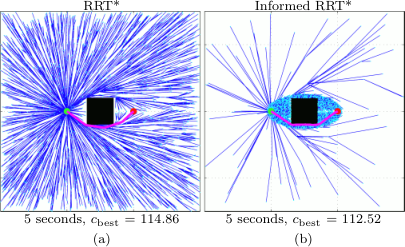
This direct-sampling method allows for the creation of informed-sampling planners. Such a planner, Informed RRTstar, is presented to demonstrate the advantages of informed incremental search (Fig. 1). Informed RRTstar behaves as RRTstar until a first solution is found, after which it only samples from the subset of states defined by an admissible heuristic to possibly improve the solution. This subset implicitly balances exploitation versus exploration and requires no additional tuning (i.e., there are no additional parameters) or assumptions (i.e., all relevant homotopy classes are searched). While heuristics may not always improve the search, their prominence in real-world planning demonstrates their practicality. In situations where they provide no additional information (e.g., when the informed subset includes the entire planning problem), Informed RRTstar is equivalent to RRTstar.

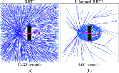
Informed RRTstar is a simple modification to RRTstar that demonstrates a clear improvement. In simulation, it performs as well as existing RRTstar algorithms on simple configurations, and demonstrates order-of-magnitude improvements as the configurations become more difficult (Fig. 2). As a result of its focused search, the algorithm has less dependence on the dimension and domain of the planning problem as well as the ability to find better topologically distinct paths sooner. It is also capable of finding solutions within tighter tolerances of the optimum than RRTstar with equivalent computation, and in the absence of obstacles can find the optimal solution to within machine zero in finite time (Fig. 3). It could also be used in combination with other algorithms, such as path-smoothing, to further reduce the search space.

The remainder of this paper is organized as follows. Section II presents a formal definition of the focused optimal planning problem and reviews the existing literature. Section III presents a closed-form estimate of the subset of states that can improve a solution for problems seeking to minimize path length in $\mathbb{R}^{n}$ and analyzes the implications on RRTstar-style algorithms. Section IV presents a method to sample this subset directly. Section V presents the Informed RRTstar algorithm and Section VI presents simulation results comparing RRTstar and Informed RRTstar on simple planning problems of various size and configuration and random problems of various dimension. Section VII concludes the paper with a discussion of the technique and some related ongoing work.

Given a positive cost function, the cost of an optimal path from $\mathbf{x}_{\rm start}$ to $\mathbf{x}_{\rm goal}$ constrained to pass through $\mathbf{x}\in X$, $f\left(\mathbf{x}\right)$, is equal to the cost of the optimal path from $\mathbf{x}_{\rm start}$ to $\mathbf{x}$, $g\left(\mathbf{x}\right)$, plus the cost of the optimal path from $\mathbf{x}$ to $\mathbf{x}_{\rm goal}$, $h\left(\mathbf{x}\right)$. As RRTstar-based algorithms asymptotically approach the optimal path to every state from above, an admissible heuristic estimate, $\widehat{f}\left(\cdot\right)$, must estimate both these terms. A sufficient condition for admissibility is that the components, $\widehat{g}\left(\cdot\right)$ and $\widehat{h}\left(\cdot\right)$, are individually admissible heuristics of $g\left(\cdot\right)$ and $h\left(\cdot\right)$, respectively.

For problems seeking to minimize path length in $\mathbb{R}^{n}$, Euclidean distance is an admissible heuristic for both terms (even with motion constraints). This informed subset of states that may improve the current solution, $X_{\widehat{f}}\supseteq X_{f}$, can then be expressed in closed form in terms of the cost of the current solution, $c_{\rm best}$, as

which is the general equation of an $n$-dimensional prolate hyperspheroid (i.e., a special hyperellipsoid). The focal points are $\mathbf{x}_{\rm start}$ and $\mathbf{x}_{\rm goal}$, the transverse diameter is $c_{\rm best}$, and the conjugate diameters are $\sqrt{c_{\rm best}^{2}-c_{\rm min}^{2}}$ (Fig. 4).

Admissibility of $\widehat{f}\left(\cdot\right)$ makes adding a state in $X_{\widehat{f}}$ a necessary condition to improve the solution. With the space-filling nature of RRT, the probability of adding such a state quickly becomes the probability of sampling such a state¹¹ 1 States may be added to $X_{\widehat{f}}$ with a sample from outside the subset until it is filled to within the RRT growth-limiting parameter, $\eta$, of its boundary.. Thus, the probability of improving the solution at any iteration by uniformly sampling a larger subset, $\mathbf{x}^{i+1}\sim\mathcal{U}\left(X_{\rm s}\right),\,X_{\rm s}\supseteq X_{\widehat{f}}$, is less than or equal to the ratio of set measures $\lambda\left(\cdot\right)$,

Using the volume of a prolate hyperspheroid in $\mathbb{R}^{n}$ gives

with $\zeta_{n}$ being the volume of a unit $n$-ball.

Uniformly distributed samples in a hyperellipsoid, $\mathbf{x}_{\rm ellipse}\sim\mathcal{U}\left(X_{\rm ellipse}\right)$, can be generated by transforming uniformly distributed samples from the unit $n$-ball, $\mathbf{x}_{\rm ball}\sim\mathcal{U}\left(X_{\rm ball}\right)$,

where $\mathbf{x}_{\rm centre}=\left(\mathbf{x}_{f1}+\mathbf{x}_{f2}\right)/2$ is the centre of the hyperellipsoid in terms of its two focal points, $\mathbf{x}_{f1}$ and $\mathbf{x}_{f2}$, and $X_{\rm ball}=\left\{\mathbf{x}\in X\;\;\middle|\;\;\left|\left|\mathbf{x}\right|\right|_{2}\leq 1\right\}$ [22].

This transformation can be calculated by Cholesky decomposition of the hyperellipsoid matrix, $\mathbf{S}\in\mathbb{R}^{n\times n}$,

where

with $\mathbf{S}$ having eigenvectors corresponding to the axes of the hyperellipsoid, $\left\{\mathbf{a}_{i}\right\}$, and eigenvalues corresponding to the squares of its radii, $\left\{r_{i}^{2}\right\}$. The transformation, $\mathbf{L}$, maintains the uniform distribution in $X_{\rm ellipse}$ [23].

For prolate hyperspheroids, such as $X_{\widehat{f}}$, the transformation can be calculated from just the transverse axis and the radii. The hyperellipsoid matrix in a coordinate system aligned with the transverse axis is the diagonal matrix

with a resulting decomposition of

where $\diag\left\{\cdot\right\}$ denotes a diagonal matrix.

The rotation from the hyperellipsoid frame to the world frame, $\mathbf{C}\in SO\left(n\right)$, can be solved directly as a general Wahba problem [24]. It has been shown that a valid solution can be found even when the problem is underspecified [25]. The rotation matrix is given by

where $\det\left(\cdot\right)$ is the matrix determinant and $\mathbf{U}\in\mathbb{R}^{n\times n}$ and $\mathbf{V}\in\mathbb{R}^{n\times n}$ are unitary matrices such that $\mathbf{U}\boldsymbol{\Sigma}\mathbf{V}^{T}\equiv\mathbf{M}$ via singular value decomposition. The matrix $\mathbf{M}$ is given by the outer product of the transverse axis in the world frame, $\mathbf{a}_{1}$, and the first column of the identity matrix, $\mathbf{1}_{1}$,

where

A state uniformly distributed in the informed subset, $\mathbf{x}_{\widehat{f}}\sim\mathcal{U}\left(X_{\widehat{f}}\right)$, can thus be calculated from a sample drawn uniformly from a unit $n$-ball, $\mathbf{x}_{\rm ball}\sim\mathcal{U}\left(X_{\rm ball}\right)$, through a transformation (5), rotation (6), and translation,

This procedure is presented algorithmically in Alg. 2.

An example algorithm using direct informed sampling, Informed RRTstar, is presented in Algs. 1 and 2. It is identical to RRTstar as presented in [8], with the addition of lines 1, 1, 1, 1, and 1. Like RRTstar, it searches for the optimal path, $\sigma^{*}$, to a planning problem by incrementally building a tree in state space, $\mathcal{T}=\left(V,E\right)$, consisting of a set of vertices, $V\subseteq X_{\rm free}$, and edges, $E\subseteq X_{\rm free}\times X_{\rm free}$. New vertices are added by growing the graph in free space towards randomly selected states. The graph is rewired with each new vertex such that the cost of the nearby vertices are minimized.

The algorithm differs from RRTstar in that once a solution is found, it focuses the search on the part of the planning problem that can improve the solution. It does this through direct sampling of the ellipsoidal heuristic. As solutions are found (line 1), Informed RRTstar adds them to a list of possible solutions (line 1). It uses the minimum of this list (line 1) to calculate and sample $X_{\widehat{f}}$ directly (line 1). As is conventional, we take the minimum of an empty set to be infinity. The new subfunctions are described below, while descriptions of subfunctions common to RRTstar can be found in [8]:

Sample: Given two poses, $\mathbf{x}_{\rm from},\,\mathbf{x}_{\rm to}\in X_{\rm free}$ and a maximum heuristic value, $c_{\rm max}\in\mathbb{R}$, the function $\mathtt{Sample}\left(\mathbf{x}_{\rm from},\mathbf{x}_{\rm to},c_{\rm max}\right)$ returns iid (iid) samples from the state space, $\mathbf{x}_{\rm new}\in X$, such that the cost of an optimal path between $\mathbf{x}_{\rm from}$ and $\mathbf{x}_{\rm to}$ that is constrained to go through $\mathbf{x}_{\rm new}$ is less than $c_{\rm max}$ as described in Section III and Alg. 2. In most planning problems, $\mathbf{x}_{\rm from}\equiv\mathbf{x}_{\rm start}$, $\mathbf{x}_{\rm to}\equiv\mathbf{x}_{\rm goal}$, and lines 2 to 2 of Alg. 2 can be calculated once at the start of the problem.

InGoalRegion: Given a pose, $\mathbf{x}\in X_{\rm free}$, the function $\mathtt{InGoalRegion}\left(\mathbf{x}\right)$ returns $\mathtt{True}$ if and only if the state is in the goal region, $X_{\rm goal}$, as defined by the planning problem, otherwise it returns $\mathtt{False}$. One common goal region is a ball of radius $r_{\rm goal}$ centred about the goal, i.e.,

RotationToWorldFrame: Given two poses as the focal points of a hyperellipsoid, $\mathbf{x}_{\rm from},\,\mathbf{x}_{\rm to}\in X$, the function $\mathtt{RotationToWorldFrame}\left(\mathbf{x}_{\rm from},\mathbf{x}_{\rm to}\right)$ returns the rotation matrix, $\mathbf{C}\in SO\left(n\right)$, from the hyperellipsoid-aligned frame to the world frame as per (6). As previously discussed, in most planning problems this rotation matrix only needs to be calculated at the beginning of the problem.

SampleUnitNBall: The function, $\mathtt{SampleUnitNBall}$ returns a uniform sample from the volume of an $n$-ball of unit radius centred at the origin, i.e. $\mathbf{x}_{\rm ball}\sim\mathcal{U}\left(X_{\rm ball}\right)$.

Informed RRTstar was compared to RRTstar on a variety of simple planning problems (Figs. 5 to 7) and randomly generated worlds (e.g., Figs. 1, 2). Simple problems were used to test specific challenges, while the random worlds were used to provide more challenging problems in a variety of state dimensions.

Fig. 5(a) was used to examine the effects of the problem range and the ability to find paths within a specified tolerance of the true optimum, with the width of the obstacle, $w$, selected randomly. Fig. 5(b) was used to demonstrate Informed RRTstar’s ability to find topologically distinct solutions, with the position of the narrow passage, $y_{g}$, selected randomly. For these toy problems, experiments were ended when the planner found a solution cost within the target tolerance of the optimum. Random worlds, as in Fig. 2, were used to test Informed RRTstar on more complicated problems and in higher state dimensions by giving the algorithms $60$ seconds to improve their initial solutions. For each variation of every experiment, $100$ different runs of both RRTstar and Informed RRTstar were performed with a common pseudo-random seed and map.

The algorithms share the same unoptimized code, allowing for the comparison of relative computational time²² 2 Experiments were run in Ubuntu 12.04 on an Intel i5-2500K CPU with 8GB of RAM.. While further optimization would reduce the effect of graph size on the computational cost and reduce the difference between the two planners, as they have approximately the same cost per iteration it will not effect the order. To minimize the effects of the steer parameter on our results, we set it equal to the RRTstar rewiring radius at each iteration calculated from $\gamma_{\rm RRT}=1.1\gamma_{\rm RRT}^{*}$, a choice we found improved the performance of RRTstar. As discussed in Section V-A, for Informed RRTstar we calculated the rewiring radius for the subproblem defined by the current solution using the expression in [8].

Experiments varying the width of the problem range, $l$, while keeping a fixed distance between the start and goal show that Informed RRTstar finds a suitable solution in approximately the same time regardless of the relative size of the problem (Fig. 8). As a result of considering only the informed subset once an initial solution is found, the size of the search space is independent of the planning range (Fig. 6). In contrast, the time needed by RRTstar to find a similar solution increases as the problem range grows as proportionately more time is spent searching states that cannot improve the solution (Fig. 8).

Experiments varying the target solution cost show that Informed RRTstar is capable of finding near-optimal solutions in significantly fewer iterations than RRTstar (Fig. 9). The direct sampling of the informed subset increases density around the optimal solution faster than global sampling and therefore increases the probability of improving the solution and further focusing the search. In contrast, RRTstar has uniform density across the entire planning domain and improving the solution actually decreases the probability of finding further improvements (Fig. 6).

Experiments varying the height of $h_{g}$ in Fig. 5(b) demonstrate that Informed RRTstar finds difficult passages that improve the current solution, regardless of their homotopy class, quicker than RRTstar (Fig. 10). Once again, the result of considering only the informed subset is an increased state density in the region of the planning problem that includes the optimal solution. Compared to global sampling, this increases the probability of sampling within difficult passages, such as narrow gaps between obstacles, decreasing the time necessary to find such solutions (Fig. 7).

Finally, experiments on random worlds demonstrate that the improvements of Informed RRTstar apply to a wide range of planning problems and state dimensions (Fig. 11).

In this paper, we discuss that a necessary condition for RRTstar algorithms to improve a solution is the addition of a state from a subset of the planning problem, $X_{f}\subseteq X$. For problems seeking to minimize path length in $\mathbb{R}^{n}$, this subset can be estimated, $X_{\widehat{f}}\supseteq X_{f}$, by a prolate hyperspheroid (a special type of hyperellipsoid) with the initial and goal states as focal points. It is shown that the probability of adding a new state from this subset through rejection sampling of a larger set becomes arbitrarily small as the dimension of the problem increases, the size of the sampled set increases, or the solution approaches the theoretical minimum. A simple method to sample $X_{\widehat{f}}$ directly is presented that allows for the creation of informed-sampling planners, such as Informed RRTstar. It is shown that Informed RRTstar outperforms RRTstar in the ability to find near-optimal solutions in finite time regardless of state dimension without requiring any assumptions about the optimal homotopy class.

Informed RRTstar uses heuristics to shrink the planning problem to subsets of the original domain. This makes it inherently dependent on the current solution cost, as it cannot focus the search when the associated prolate hyperspheroid is larger than the planning problem itself. Similarly, it can only shrink the subset down to the lower bound defined by the optimal solution. We are currently investigating techniques to focus the search without requiring an initial solution. These techniques, such as BITstar (BITstar) [26], incrementally increase the search subset. By doing so, they prioritize the initial search of low-cost solutions.

An OMPL (OMPL) implementation of Informed RRTstar is described at http://asrl.utias.utoronto.ca/code.

This research was funded by contributions from the NSERC (NSERC) through the NCFRN (NCFRN), the Ontario Ministry of Research and Innovation’s Early Researcher Award Program, and the ONR (ONR) Young Investigator Program.

References

- [2] P. E. Hart, N. J. Nilsson, and B. Raphael, “A formal basis for the heuristic determination of minimum cost paths,” TSSC, 4(2): 100–107, Jul. 1968
- [3] S. M. LaValle and J. J. Kuffner Jr., “Randomized kinodynamic planning,” IJRR, 20(5): 378–400, 2001.
- [4] L. E. Kavraki, P. Švestka, J.-C. Latombe, and M. H. Overmars, “Probabilistic roadmaps for path planning in high-dimensional configuration spaces,” TRA, 12(4): 566–580, 1996.
- [5] D. Hsu, R. Kindel, J.-C. Latombe, and S. Rock, “Randomized kinodynamic motion planning with moving obstacles,” IJRR, 21(3): 233–255, 2002.
- [6] C. Urmson and R. Simmons, “Approaches for heuristically biasing RRT growth,” IROS, 2: 1178–1183, 2003.
- [7] D. Ferguson and A. Stentz, “Anytime RRTs,” IROS, 5369–5375, 2006.
- [8] S. Karaman and E. Frazzoli, “Sampling-based algorithms for optimal motion planning,” IJRR, 30(7): 846–894, 2011.
- [9] M. Otte and N. Correll, “C-FOREST: Parallel shortest path planning with superlinear speedup,” TRO, 29(3): 798–806, Jun. 2013
- [10] Y. Gabriely and E. Rimon, “CBUG: A quadratically competitive mobile robot navigation algorithm,” TRO, 24(6): 1451–1457, Dec. 2008.
- [11] N. Gasilov, M. Dogan, and V. Arici, “Two-stage shortest path algorithm for solving optimal obstacle avoidance problem,” IETE Jour. of Research, 57(3): 278–285, May 2011.
- [12] S. Kiesel, E. Burns, and W. Ruml, “Abstraction-guided sampling for motion planning,” SoCS, 2012.
- [13] R. Alterovitz, S. Patil, and A. Derbakova, “Rapidly-exploring roadmaps: Weighing exploration vs. refinement in optimal motion planning,” ICRA, 3706–3712, 2011.
- [14] B. Akgun and M. Stilman, “Sampling heuristics for optimal motion planning in high dimensions,” IROS, 2640–2645, 2011.
- [15] J. Nasir, F. Islam, U. Malik, Y. Ayaz, O. Hasan, M. Khan, and M. S. Muhammad, “RRT*-SMART: A rapid convergence implementation of RRT*,” Int. Jour. of Adv. Robotic Systems, 10, 2013.
- [16] D. Kim, J. Lee, and S. Yoon, “Cloud RRT*: Sampling cloud based RRT*,” ICRA, 2014.
- [17] S. Karaman, M. R. Walter, A. Perez, E. Frazzoli, and S. Teller, “Anytime motion planning using the RRT*,” ICRA, 1478–1483, 2011.
- [18] M. Jordan and A. Perez, “Optimal bidirectional rapidly-exploring random trees,” CSAIL, MIT, MIT-CSAIL-TR-2013-021, 2013.
- [19] O. Arslan and P. Tsiotras, “Use of relaxation methods in sampling-based algorithms for optimal motion planning,” ICRA, 2013.
- [20] S. Koenig, M. Likhachev, and D. Furcy, “Lifelong planning A*,” Artificial Intelligence, 155(1–2): 93–146, 2004.
- [21] J. D. Gammell, S. S. Srinivasa, and T. D. Barfoot, “On recursive random prolate hyperspheroids,” Autonomous Space Robotics Lab, University of Toronto, TR-2014-JDG002, 2014. arXiv:1403.7664 [math.ST]
- [22] H. Sun and M. Farooq, “Note on the generation of random points uniformly distributed in hyper-ellipsoids,” in Fifth Int. Conf. on Information Fusion, 1: 489–496, 2002.
- [23] J. D. Gammell, and T. D. Barfoot, “The probability density function of a transformation-based hyperellipsoid sampling technique,” Autonomous Space Robotics Lab, University of Toronto, TR-2014-JDG004, 2014. arXiv:1404.1347 [math.ST]
- [24] G. Wahba, “A least squares estimate of satellite attitude,” SIAM Review, 7: 409, 1965.
- [25] A. H. J. de Ruiter and J. R. Forbes, “On the solution of Wahba’s problem on SO(n),” Jour. of the Astronautical Sciences, 2014, to appear.
- [26] J. D. Gammell, S. S. Srinivasa, and T. D. Barfoot, “BIT*: Batch informed trees for optimal sampling-based planning via dynamic programming on implicit random geometric graphs,” Autonomous Space Robotics Lab, University of Toronto, TR-2014-JDG006, 2014. arXiv:1405.5848 [cs.RO]