Linear stability of magnetized massive protoplanetary disks
Abstract
Magneto-rotational instability (MRI) and gravitational instability (GI) are the two principle routes to turbulent angular momentum transport in accretion disks. Protoplanetary disks may develop both. This paper aims to reinvigorate interest in the study of magnetized massive protoplanetary disks, starting from the basic issue of stability. The local linear stability of a self-gravitating, uniformly magnetized, differentially rotating, three-dimensional stratified disk subject to axisymmetric perturbations is calculated numerically. The formulation includes resistivity. It is found that the reduction in the disk thickness by self-gravity can decrease MRI growth rates; the MRI becomes global in the vertical direction, and MRI modes with small radial length scales are stabilized. The maximum vertical field strength that permits the MRI in a strongly self-gravitating polytropic disk with polytropic index is estimated to be , where is the midplane sound speed and is the angular velocity. In massive disks with layered resistivity, the MRI is not well-localized to regions where the Elsasser number exceeds unity. For MRI modes with radial length scales on the order of the disk thickness, self-gravity can enhance density perturbations, an effect that becomes significant in the presence of a strong toroidal field, and which depends on the symmetry of the underlying MRI mode. In gravitationally unstable disks where GI and MRI growth rates are comparable, the character of unstable modes can transition smoothly between MRI and GI. Implications for non-linear simulations are discussed briefly.
I. Introduction
Astrophysical disks host a wide range of fluid instabilities. Among them, the magneto-rotational instability [11, 5, 6, MRI,] and gravitational instability [55, 25, 26, GI, ] provide robust pathways to turbulent angular momentum transport that enables mass accretion [7, 3, 56, and references therein]. They are also relevant to planet formation theory. For example, the strength of MRI turbulence directly affect planetesimal dynamics in protoplanetary disks [58, 29]; while GI can potentially form giant planets directly through disk fragmentation [9, 10, 23, 57, 30].
Accretion disks such as those surrounding black holes can develop both MRI and GI [46, 27]. Protoplanetary disks (PPDs) are also expected to be massive and magnetized in its earliest evolutionary phase [31]. The interplay between MRI and GI has been invoked to explain outbursts in circumstellar disks [4, 60, 59, 45], and predicts similar phenomenon in circumplanetary disks [41]. This results from the development of ‘dead zones’ — magnetically inactive, laminar regions near the disk midplane — with magnetized layers above and below [21, 44, 38]. Mass accumulation in the dead zone can lead to GI and trigger MRI through heating. In these models, the condition required for MRI is realized through GI, but the MRI is unaffected by disk self-gravity.
PPDs subject to both MRI and GI are often modeled through separate turbulent viscosity coefficients in a hydrodynamical framework [54]. This implicitly assumes that the development of MRI and GI can be assessed independently. Circumstellar disk models that explicitly combine the equations of magneto-hydrodynamics and self-gravity have been limited to a few early simulations [19, 17, 16]. It will be necessary to revisit and extend these pioneering calculations to fully explore the impact of MRI and GI on the structure and evolution of PPDs. In preparation of this, it is important to have a thorough understanding of the stability properties of such systems.
Since compressibility is not fundamental for the MRI, much of the early stability calculations assume incompressible perturbations [28, 32]. However, recent works indicate compressibility may be important under certain conditions, such as strong fields [34, 51, 8]. Previous MRI studies have also focused on modes with vanishing radial wavenumber, because they are the most unstable [53, 52]. Self-gravity has minimal effect on such perturbations in a rotating disk. However, modes with radial length scales on the order of the disk scale height may be subject to self-gravity. It is therefore of interest to generalize the MRI with non-zero radial wavenumbers to massive disks.
The effect of a magnetic field on the GI of rotating disks has been considered recently by [40], who generalized the Toomre stability criterion for razor-thin disks to include a vertical field. For circumstellar disks, the authors concluded that the field is stabilizing. This is consistent with previous analysis by [47] for three-dimensional (3D) uniformly rotating disks. However, the GI of 3D differentially rotating disks have mostly neglected magnetic fields [43, 33], but such disks are subject to the MRI if magnetized.
This work marks the beginning of our study of magnetized, self-gravitating PPDs. We start from linear calculations, which have the advantage that a wide range of parameters can be studied at negligible computational cost. This allows us to identify conditions, if any, under which MRI and GI cannot be considered independent. It is also important to have such calculations to benchmark and guide future non-linear simulations.
This paper is organized as follows. §II lists the governing equations and describes the disk equilibria under consideration. The linear problem is formulated in §III. The impact of self-gravity on the MRI with a vertical field is discussed in §IV, gravitationally unstable disks are considered in §V, and equilibria including an azimuthal field is explored in §VI. We summarize results in §VII with a discussion of important extensions to our current models.
II. Local disk model
We study the local stability of an inviscid, self-gravitating and magnetized fluid disk orbiting a central star with potential , where are cylindrical co-ordinates from the star. We use the shearing box approximation [26] to consider a small patch of the disk at a fiducial radius . The local frame rotates at angular velocity about the star, where . We also define as the local shear rate and as the square of the local vertical frequency.
A Cartesian co-ordinate system is set up in this local frame, corresponding to the radial, azimuthal and vertical directions of the global disk, respectively. The shearing box fluid equations read
| (1) | ||||
| (2) | ||||
| (3) |
where is the density field; is the total velocity in the local frame; is the magnetic field which satisfies ; is the total pressure, and is the vacuum permeability. We choose a barotropic equation of state, specified below, so that the gas pressure is given by . The resistivity is either uniform or a prescribed function of height.
The total potential is , where
| (4) |
is the effective external potential (central plus centrifugal) in the shearing box approximation, where and ; and the gas potential satisfies Poisson’s equation
| (5) |
where is the gravitational constant. For clarity, hereafter we drop the subscript on the frequencies.
II.1. Equilibrium disk
The unperturbed disk is steady and described by , where are constants and the toroidal field strength is . The equilibrium velocity field is . We consider Keplerian disks so that and the epicycle frequency . We assume a thin disk and neglect the radial component of the self-gravitational force in the unperturbed disk.
The equilibrium density field is obtained by solving
| (6) | ||||
| (7) |
We consider
(i) isothermal disks with ; (ii) polytropic disks with with ;where is the midplane density. The sound speed so that is the global sound speed in the isothermal disk, and is the midplane sound speed in the polytropic disk. For the polytropic disk the disk thickness is such that . Since the isothermal disk has no surface, we define such that . A non-dimensional measure of the disk thickness is given by
| (8) |
and will appear in subsequent discussions.
We solve for with boundary conditions and at . This is done numerically for isothermal disks and analytically for the polytropic disk (see Appendix A). Examples of density profiles are shown in Fig. 1. The normalized density field is weakly dependent on the strength of self-gravity provided the -axis is appropriately scaled.


II.2. Resistivity profile
We adopt constant resistivity or a resistivity prescription such that increase towards the midplane. In the latter case, we follow [15] and use the resistivity profile
| (9) |
where
| (10) | ||||
| (11) |
and , so that and . The constant is chosen such that
| (12) |
and we define as the conductivity boost factor from the midplane to the disk surface. We remark that once and are obtained from Eq. 6 — 7, the integration for Eq. 11 can be performed implicitly by using Poisson’s equation.
We use the Elsasser number a non-dimensional measure of conductivity,
| (13) |
where is the vertical Alfven speed. Because of the density stratification, the Elsasser number increases with height even for constant resistivity. The disk may be considered ideal where .
II.3. Disk parameters
The strength of self-gravity is parametrized by
| (14) |
[43], which is used to set the midplane density . A relation between and the Toomre parameter for gravitational instability of razor-thin disks, , is described in Appendix B.
The plasma measures the inverse strength of the magnetic field
| (15) |
where is the midplane Alfven speed. Note that we use the vertical field for this definition throughout this paper.
The strength of conductivity is measured by the midplane Elsasser number
| (16) |
For non-uniform resistivity we also specify .
III. Linear problem
We consider axisymmetric Eulerian perturbations to the above equilibrium in the form and similarly for other fluid variables. Here, is a constant radial wavenumber and is a complex frequency, where is the real mode frequency and is the growth rate. We take without loss of generality. Hereafter, we suppress the exponential factor and the real part notation.
The linearized continuity equation is
| (17) |
where ′ denotes and is the enthalpy perturbation. The linearized equations of motion are
| (18) | ||||
| (19) | ||||
| (20) |
where the effective enthalpy perturbation . The components of the linearized induction equation are
| (21) | ||||
| (22) | ||||
| (23) |
where , , and the divergence-free condition is . Finally, the linearized Poisson equation is
| (24) |
We eliminate and between the linearized equations to obtain a system of ordinary differential equations for . We detail the steps in Appendix C for two cases considered in this paper:
- 1.
Purely vertical field with constant or variable resistivity, so that and .
- 2.
Tilted field with uniform resistivity so that and .
Schematically, the numerical problem is to solve
| (25) | ||||
| (26) | ||||
| (27) | ||||
| (28) |
where the differential operators and () can be read off Appendix C and () from the linearized Poisson equation above. We remark that the case of a tilted field and variable resistivity can also be reduced to the above form.
III.1. Domain and boundary conditions
For a vertical field, considered in §IV and §V, we take to be an even function of . Odd modes are permitted in §VI, where an azimuthal field may be included. In both setups the gravitational potential boundary condition, given by [25], is
| (29) |
where is the vertical Lagrangian displacement, and is the upper and lower disk surfaces, respectively.
III.1.1 Case 1: vertical field
Here we impose at . This permits higher numerical resolution by reducing the computational domain to . At the upper disk boundary we set
| (30) |
so the field remains vertical. The derivation of the magnetic field boundary conditions may be found in [53].
III.1.2 Case 2: tilted field
In this more general setup the computational domain is and no symmetry across the midplane is enforced. At the disk surfaces we adopt the ‘halo’ model of [24], so that
| (31) | ||||
| (32) | ||||
| (33) |
and this case permits .
III.2. Numerical procedure
We use a pseudo-spectral method to solve the set of linearized equations. Let
| (34) |
where
| (35) |
and is a Chebyshev polynomial of the first kind of order [1]. Note that for case 1 the midplane symmetry condition is taken care of by the choice of basis functions.
The pseudo-spectral coefficients are obtained by demanding the set of linear equations to be satisfied at collocation points along the vertical direction, here chosen to be the extrema of plus end points, where is the highest polynomial order. Our standard resolution is () for case 1 (case 2).
The above procedure discretize the linear equations to a matrix equation,
| (36) |
where is a matrix representing the plus boundary conditions, and is a vector storing the pseudo-spectral coefficients. Starting with an initial guess for , non-trivial solutions to Eq. 36 are obtained by varying using Newton-Raphson iteration such that [39, details can be found in].
III.2.1 Non-dimensionalization
We solve the linearized equations in non-dimensional form, by defining
| (37) | ||||
| (38) |
where . We also non-dimensionalize background quantities, i.e. , , , and .
III.3. Diagnostics
We visualize results in terms of dimensionless energy densities. We define
| (39) | ||||
| (40) | ||||
| (41) | ||||
| (42) |
as the perturbed magnetic, gravitational, kinetic and thermal energies, respectively, which are functions of . Although we do not solve an energy equation, we nevertheless define as a measure of density perturbations [37]. The total energy is . We use to denote an average over .
Since we will primarily be concerned with massive disks, we define
| (43) |
as a measure of the importance of self-gravity. Thus, modes with are energetically dominated by self-gravity (GI) and modes with are dominated by magnetic perturbations (MRI).
IV. MRI in self-gravitating disks
In this section we focus on the MRI and use the vertical field setup of case 1. We first consider MRI modes with negligible density/potential perturbations to see the effect of self-gravity on the MRI through the background stratification, then go on to examine MRI modes with density/potential perturbations in massive disks.
IV.1. Influence of self-gravity on the MRI through the background equilibrium
Here we use polytropic disks, which have a well-defined disk thickness. The upper disk boundary is set to . We fix and unless otherwise stated.
IV.1.1 Uniform resistivity
Fig. 2 plots MRI growth rates as a function of and . The resistivity is uniform (). For ideal MHD and a weak field (, ), there is negligible dependence on . However, with or in the resistive limit (), growth rates decrease noticeably for (). Since we find density and potential perturbations to be negligible (i.e. the linear response is non-self-gravitating), this shows that disk self-gravity can affect the MRI through the background equilibrium.

[53] found that for MRI to operate, its wavelength should fit inside the disk. That is,
| (44) |
where the MRI wavelengths are given by
| (45) |
for ideal MHD, and
| (46) |
in the limit of high resistivity.
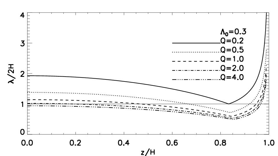
Because is weakly dependent on (Fig. 1), self-gravity only affects the MRI through the factor , which increases with decreasing (see Fig. 17 in Appendix A). This implies that sufficiently strong self-gravity can stabilize the MRI by making .
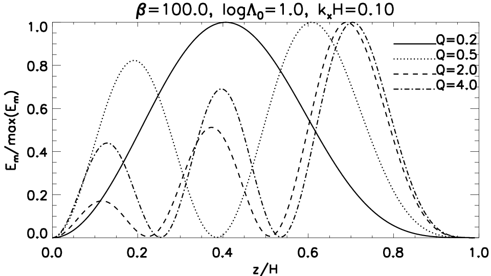
In the ideal limit with , we find throughout most of the disk for the values of considered, so self-gravity does not affect growth rates significantly. However, the ratio does increase with stronger self-gravity. Consequently, the wavelength of the instability, in units of , increases. This is shown in Fig. 3 which plots the magnetic energies for and a range of values. The number of vertical nodes decrease with , i.e. the disk accommodates fewer wavelengths because increasing vertical self-gravity makes it thinner.
We repeated the case with a stronger field , shown in Fig. 2 as the dashed-triple dot line. Here, strong self-gravity is effective in reducing the growth rate, because decreasing enhances the dependence of on . For and we find at the midplane and the growth rate is reduced significantly.
Self-gravity also appreciably decreases the MRI growth rates in the resistive limit. Fig. 4 plots Eq. 44 for . In the non-self-gravitating disk () the instability criterion is marginally satisfied and the MRI operates. As decreases, Eq. 44 is violated and the MRI growth rate is significantly reduced. This is seen for where throughout the disk. (The instability is not suppressed since Eq. 45—46 is only exact for unstratified disks.) Although the function does not change significantly for the range of considered, the dependence of on is amplified by the denominator in the resistive case. Modes in Fig. 4 have no nodes in the magnetic energy except at , i.e. only the longest wavelength survives against large resistivity.
IV.1.2 Layered resistivity
Here we consider disks with midplane Elsasser number and a variable resistivity profile with . Fig. 5 compares the magnetic energies for and . They have similar growth rates, and , respectively. In the non-self-gravitating limit (), the MRI is effectively suppressed for . This is consistent with the picture of layered accretion proposed for non-self-gravitating disks [21, 15]. However,in the massive disk () the mode occupies a wider vertical extent because its wavelength (in units of ) is larger. This suggests that in massive disks, the MRI is not well localized to a sub-layer within the height, even when the resistivity has a layered structure.
We also performed additional calculations with and [29, see Fig. 1 of ]. For , we find no significant increase in the magnetic energy in the resistive zones. However, lowering gives similar results to Fig. 5, e.g. for and or and the magnetic energy penetrates into the resistive zone for strongly self-gravitating disks. In general, the magnetic energy density maximum moves toward the midplane with increasing self-gravity.

IV.1.3 Dependence on
The above experiments show that with increasing disk self-gravity, the MRI becomes more global in the vertical direction. We find a similar result in the horizontal direction. Fig. 6 show MRI growth rates as a function of for a range of values. Increasing self-gravity decreases the cut-off radial wavenumber for the MRI. We checked that these modes have negligible density perturbations. Then we can understand this result by invoking the instability criteria for incompressible MRI in an unstratified Keplerian disk,
| (47) |
where is a vertical wavenumber [34]. Setting and non-dimensionalizing, we find
| (48) |
where order-unity factors have been dropped. Despite a simplistic approach, this demonstrates that with increasing self-gravity (increasing ), we expect MRI modes with small radial length scales to be suppressed.

IV.2. Influence of self-gravity on the MRI through the linear response
Our goal here is to examine whether or not self-gravity can amplify the density perturbations associated with the MRI. We compute unstable modes in a massive isothermal disk with (corresponding to ), which is still expected to be marginally stable to gravitational instability [43, who find a critical value of ]. The upper disk boundary is set to .
IV.2.1 Ideal disks
We first consider ideal MHD by adopting a uniform resistivity with . Fig. 7 plots MRI growth rates as a function of for several values of . The curves are color-coded according . (Recall implies self-gravity dominates over magnetic perturbations, and is the opposite limit.) The potential perturbation is negligible for all cases when , since the MRI becomes incompressible as .

For , i.e. a weak field, density perturbations are negligible and the incompressible MRI operates. However, as is lowered and the MRI growth rate reduced, we find non-negligible potential perturbation for . This suggests that in a strongly magnetized disk that still permits the MRI, the associated density perturbation can be important when the disk is self-gravitating.
IV.2.2 Resistive disks
We repeat the above calculation for resistive disks, but fix and vary the midplane Elsasser number . Growth rates are shown in Fig. 8. Interestingly, the highly resistive case has comparable magnetic and gravitational energies: at we find , which corresponds to . Fig. 9 compares the magnetic energy of this mode to that computed in the Cowling approximation, where the Poisson equation is ignored in the linearized equations and the potential perturbation set to zero (formally letting in Eq. 24). The growth rate increases when self-gravity is included in the linear response, since self-gravity is usually destabilizing. However, and are very similar, indicating that the instability in the self-gravitating calculation is fundamentally still the MRI.


Fig. 10 plots the energies associated with the MRI mode discussed above. The gravitational energy exceeds the magnetic energy near the midplane (). The growth rate is not much smaller than that of the most unstable mode ( for ), so significant density perturbations will grow on dynamical timescales for this system, even though GI is not expected.

IV.2.3 Qualitative interpretation
To make sense of the above results, we first return to ideal MHD and consider regions close to the disk midplane (), where self-gravity is expected to be most important. For this discussion we will ignore stratification and set . The governing equations are then
| (49) | ||||
| (50) | ||||
| (51) | ||||
| (52) |
where . We imagine an iterative procedure to solve the above equations, starting from the Cowling approximation where and . This is the standard MRI and we denote the solution as , and . Eq. 51 implies
| (53) |
We argue below that by taking . Then, recalling , we can write
| (54) |
The MRI has, in general, a non-zero density perturbation. However, it is negligible for and/or a weak field ().
We now include self-gravity. The Poisson equation implies has an associated potential perturbation,
| (55) |
Physically, we expect , so that a positive (negative) local density perturbation causes a negative (positive) local potential perturbation. We then insert back into the momentum and continuity equations, and ask how does this potential perturbation modify the Cowling solution? Writing and similarly for and , we find
| (56) | ||||
| (57) | ||||
| (58) |
Now, if the perturbations to the magnetic field remain unchanged, i.e. the mode remains close to the standard MRI as observed in Fig. 9, then and , so Eq. 57 is satisfied. Eq. 56 then require . This is compatible with Eq. 58 if
| (59) |
For the ideal MRI, we take . Then because and we are considering . Thus Eq. 59 is generally satisfied.
The above assumptions imply
| (60) |
which indicates a non-zero density perturbation due to the MRI can be amplified by self-gravity. Now, for we have because and for the cases considered above. Then
| (61) |
suggesting stronger amplification of the density field by self-gravity with increasing field strength (decreasing ).
The above arguments can be adapted to the resistive disk. Eq. 51—52 are unchanged, while resistive terms appearing in Eq. 49—50 only involve the potential perturbation through . For the resistive MRI we take and [53]. Then so Eq. 59 is satisfied. Noting that , the feedback equation becomes
| (62) |
so increasing the resistivity (decreasing ) should enhance density perturbations.
For weak fields in an ideal disk, the MRI has a vertical wavelength . It will be almost incompressible so the ‘seed’ density perturbation is small. The perturbed mass contained within is small and its potential is unimportant. Furthermore, considering the stratified disk, imply rapid variations in the density perturbation across the disk height, averaging to zero, so the magnitude of the associated potential perturbation is small. Self-gravity does not affect the MRI in this regime.
However, a strong field and/or large resistivity increases the MRI vertical wavelength. When the vertical scale of the MRI becomes comparable to the disk thickness, i.e. , the perturbed mass across the disk height can contribute to a net potential perturbation. We therefore expect a necessary condition for self-gravity to affect the MRI is for the latter to be weak.
V. Gravitationally unstable disks
Gravitational instability becomes possible in a sufficiently massive and/or cold disk. Here, we explore whether or not GI and MRI can interact by computing unstable modes for isothermal disks with () which permits GI, as shown below. We consider ideal disks with and , unless otherwise stated.
V.1. Co-existence of MRI and GI
Fig. 11 show growth rates for modes with as a function of in disks with , and . All three cases display distinct GI modes (red/brown branch). The GI growth rates are for , respectively. GI is stabilized by magnetic pressure for sufficiently small . The critical field strength for stabilizing GI increases with increasing self-gravity, consistent with [47]. For , GI is stabilized for . Nevertheless, the MRI branch for becomes self-gravitating, so that density perturbations still grow, even though GI does not formally operate.


The GI and MRI branches only interact when their growth rates are similar. This is seen in Fig. 11 for where the GI branch approaches a MRI branch at . In fact, following the red curve to smaller indicates GI transitions to MRI. The ‘gaps’ in the GI and MRI branches for and may be due to the phenomenon of avoided crossing, as seen in stars [2, e.g.] and accretion tori/disks [12, 48, e.g.], where physically distinct modes approach one another in frequency and exchange character. However, we cannot exclude the possibility that some modes may have been missed in a numerical search of eigenfrequencies.
Thus, our results do not rigorously prove that the GI and MRI branches do not intersect. Nevertheless, the continuous variation of strongly suggest that unstable modes can transition smoothly from MRI to GI and vice versa, especially at low .
V.1.1 Case study
In reality, perturbations with a range of will be present for a given set of disk parameters. Fig. 12 show growth rates as a function of in a disk with , where MRI and GI have comparable growth rates. All perturbations with grow dynamically (, or 1.6 orbits).
We also plot in Fig. 12 growth rates obtained from the Cowling approximation, which isolates MRI; and that from a high-resistivity run, which isolates GI by allowing the field lines to slip through the fluid. We refer to these as pure MRI and pure GI, respectively. For , growth rates are equal to those on the pure MRI and pure GI branches. That is, MRI and GI operate independently until their growth rates become equal as a function of .
The dispersion relation deviates from the pure GI/MRI curves with increasing , implying stronger interaction between magnetic and density perturbations. Comparing pure GI (dashed line) and the gravitationally-dominated portions of shows that inclusion of magnetic field stabilizes high- pure GI. (Note also the slight decrease in the most unstable .) This stabilization is due to magnetic pressure [40], consistent with pressure stabilizing small-wavelength GI only.
Comparing pure MRI (solid line) and the magnetically-dominated portions of show that self-gravity increases MRI growth rates at large . This effect is small but noticeable, which can be used as a code test for non-linear simulations. Note that this destabilization by self-gravity is through the linear response, rather than through the background stratification (which is stabilizing).

VI. Effect of an azimuthal field
In this section we use the setup of case 2 described in §III, and examine the effect of an azimuthal field so that , parametrized by . However, we continue to use for normalizations and is associated with the vertical Alfven speed. We also extend the previous calculations to the full disk , which allows us to compare the effect of self-gravity on MRI modes with different symmetries across the midplane. We use an isothermal disk throughout.
VI.1. Ideal disks with MRI
We consider disks with () and in the limit of ideal MHD (). Gravitational instability is not expected because Fig. 11 shows that even for , GI is suppressed for .
Fig. 13 show MRI growth rates for and . We divide the modes into two categories depending on the extremum of magnetic energy at the midplane. The top panel are modes where has a local minimum at and the bottom panel are modes where has a local maximum at . The latter set of modes were excluded in the previous sections by midplane boundary conditions. We also plot growth rates computed in the Cowling approximation. As expected, , so none of the modes are energetically dominated by self-gravity.


Consider first modes in the top panel of Fig. 13. As with previous results, self-gravity destabilizes modes with . Consequently, the cut-off wavenumber is larger when SG is included. Destabilization is most effective for purely vertical fields: with , SG increases the growth rate by . For we find the density perturbation is an even function. Although these modes are fundamentally magnetic, this is consistent with [25], who showed that SG can only destabilize symmetric density perturbations. With increasing , we find deviates from an even function. Together with the increased total magnetic pressure with (since is fixed), destabilization by SG weakens. Thus, the Cowling approximation becomes increasingly good with stronger for these modes.
The modes in the bottom panel of Fig. 13 display opposite behavior. For we find is odd, and self-gravity has no effect. When , deviates from an odd function and the midplane density perturbation increases. SG is stabilizing for these modes at all wavelengths, and is most effective at . Fig. 14 show eigenfunctions for and with and without the Cowling approximation. SG significantly enhances the midplane density perturbation, making the gravitational potential energy comparable to the magnetic energy, which becomes more confined near the midplane.


To interpret the above result for modes with magnetic energy concentrated at the midplane, we note that compressibility affects the MRI in the presence of an azimuthal field even in a non-self-gravitating disk. If the perturbed disk remains in vertical hydrostatic equilibrium, then
| (63) |
to order of magnitude in a non-SG disk. Thus a strong azimuthal field can cause a large density perturbation [51]. We checked that for the modes in Fig. 14, vertical velocities are small, .
Compressibility is enhanced by an azimuthal field, which is stabilizing for the MRI [34]. This effect is significant for because the azimuthal Alfven speed is sonic. Fig. 14 indicates that self-gravity further enhances compressibility, and therefore stabilization. We suspect this is overwhelmed by the destabilization effect of SG, because the density perturbation has an anti-symmetric component.
VI.2. Resistive disks with GI
Here we examine a resistive disk which permits MRI and GI by setting , and . Fig. 15 show growth rates for and . For , MRI and GI are decoupled except for a narrow range of in which the lower MRI modes transitions to GI. Notice that the upper MRI modes intersect the GI branch. There is no interaction because the upper MRI modes have anti-symmetric whereas the GI modes have symmetric .


Introducing leads to an exchange in the mode characters. For the modes on the two MRI branches are similar to the vertical field case. However, for the upper MRI mode transitions to GI, for which is a minimum; and the lower MRI mode has being a maximum. We find all perturbations with have symmetric .
Increasing the azimuthal field further to we find overstable MRI modes with non-negligible real frequencies [21]. An example is shown in Fig. 16. Notice the density/potential perturbation is off-set from the midplane. This is not possible for pure GI [25]. Thus, these overstable MRI modes indeed become self-gravitating, before being stabilized.
Notice also in Fig. 15 the disappearance of magnetic modes between as is increased. For , MRI and GI are again independent because they operate at distinct radial scales. This implies that perturbations unstable to GI cannot develop MRI.

VII. Summary and discussion
In this paper, we have performed axisymmetric linear stability calculations of magnetized, self-gravitating, vertically stratified disks in the local approximation. Our models include resistivity and azimuthal fields. We have identified regimes under which the magneto-rotational instability (MRI) is affected by disk self-gravity (SG).
For a vertical field, the requirement for the MRI to operate is that its vertical wavelength . The disk thickness decreases with increasing SG. This reduces MRI growth rates when , and hence , is fixed. Thus, a sufficiently massive disk can potentially suppress the MRI. The MRI is also restricted to larger radial scales as is lowered. This means that the MRI becomes more global in self-gravitating disks.
The condition may be written more precisely as
| (64) |
where is a numerical factor and accounts for the ideal and resistive limits (see Eq. 45—46). Since increases with decreasing , Eq. 64 implies the MRI requires larger values of with increasing self-gravity. For definiteness, consider the ideal polytropic disk. Then Eq. 64 is
| (65) |
For a non-self-gravitating disk, and Eq. 65 is . For , the condition is , giving for . We confirm this numerically, finding the MRI growth rate when for and for .
We can also place an upper bound on the absolute field strength . Writing , we find Eq. 65 is independent of for , and
| (66) |
is needed for the MRI to operate in the ideal polytropic disk with strong self-gravity. Although both the MRI wavelength and disk thickness vanish as , the MRI can still operate provided the field is sufficiently weak according to Eq. 66.
Interestingly, for layered resistivity we do not find layered magnetic perturbations when the disk is massive. This is consistent with the MRI becoming vertically global with increasing self-gravity. For non-self-gravitating disks , so the MRI can be restricted to regions of size , i.e. an active layer. This not compatible with , as found for massive disks. Hence we find magnetic perturbations penetrate into the high-resistivity dead zone (e.g. in Fig. 5), and there is no distinct boundary between active and dead layers. This suggests that the picture of layered accretion [15, e.g.] may not be applicable to self-gravitating disks.
We find MRI modes with radial scales of can acquire density perturbations in massive but Toomre-stable disks. This occurs when the MRI is weak, for example with a strong field or high resistivity. We argue in that case , so the MRI is compressible and the associated density perturbation can be enhanced by self-gravity.
At this point it is worth mentioning previous non-linear simulations of magnetized self-gravitating galactic and circumstellar disks [36, 20, 19]. These authors find self-gravity did not enhance MRI density fluctuations significantly. However, they employed ideal MHD simulations with gas-to-magnetic pressure ratios of order to . This is qualitatively consistent with our results, as self-gravity is not expected to influence the MRI in this regime of , except through the background state. For example, [19] found MRI turbulence is more coherent in self-gravitating disks. This may be related to our finding that small radial scale MRI is suppressed when self-gravity is included in the background equilibria.
Physically, we expect MRI to interact with self-gravity when their spatial scales are similar. Because self-gravity acts globally in the vertical direction, for it to affect the MRI, future non-linear simulations should consider parameter regimes in which the MRI is vertically global. Indeed, in the setup of [36], the disk scale height exceeds the MRI vertical wavelength and self-gravity has little impact.
Curiously, when GI and MRI are simultaneously supported, we find unstable modes transition between MRI and GI. There exists modes with comparable potential and magnetic energy perturbations, which demonstrates MRI and GI can interact. These transitions occur smoother with decreasing (Fig. 11) or increasing (Fig. 12). The latter implies that, in order to capture the magneto-gravitational interactions represented by these intermediate modes, non-linear simulations must resolve radial scales smaller than the most unstable GI mode. For example, Fig. 12 suggest radial scales down to should be well-resolved.
We examined the effect of an additional azimuthal field, while keeping the vertical field at fixed strength. In this case, we also relaxed the equatorial symmetry condition applied previously and considered the full disk column. Self-gravity affects the MRI differently depending on its character. Self-gravity destabilizes MRI modes where the magnetic energy has a minimum at , these modes have a symmetric density perturbation in the limit . However, self-gravity stabilizes MRI modes where the magnetic energy has a maximum at , these modes have an anti-symmetric density perturbation in the limit . This stabilization effect is stronger for increasing . Previous linear calculations show that increased compressibility associated with a toroidal field stabilizes the MRI [36]. We conjecture that self-gravity further enhances this effect. Non-linear MRI simulations with strong toroidal fields that neglect self-gravity may over-estimate the strength of MRI turbulence.
VII.1. Caveats and outlooks
We discuss below two major extensions to our linear model that should be undertaken, before embarking on non-linear simulations of magnetized, self-gravitating disks, which is our eventual goal.
Beyond the shearing box. The shearing box ignores the curvature of toroidal field lines present in the global disk geometry. [51] demonstrated new effects on the MRI when the curvature of a super-thermal toroidal field is accounted for; although Pessah & Psaltis focused on modes with large (small) vertical (radial) wavenumbers, for which we expect self-gravity can be ignored. Since compressibility becomes important for strong toroidal fields, the effect of self-gravity on modes with may become significant when super-thermal toroidal fields are considered. However, global disk models will be necessary to self-consistently probe this regime.
Beyond axisymmetry. Axisymmetric perturbations, as we have assumed, preclude gravitational torques [42]. The local non-axisymmetric stability of magnetized self-gravitating thin disks has been considered by several authors [13, 22, 14, 35]. However, two-dimensional models exclude the MRI. It will be necessary to generalize these studies to 3D in order to investigate the impact of the MRI on angular momentum transport by gravitational instability. Furthermore, self-gravitating disks can develop global spiral instabilities while stable against local axisymmetric perturbations [50, 49]. Global non-axisymmetric linear models will be desirable to support non-linear simulations of this kind [18, 16].
Appendix A Analytic equilibrium for the polytropic disk
For a polytropic disk with the dimensional equilibrium equation to be solved is
| (A1) |
which is obtained by combining Eq. 6 and 7 with the above equation of state. The solution is
| (A2) |
where
| (A3) |
The polytropic disk thickness is
| (A4) |
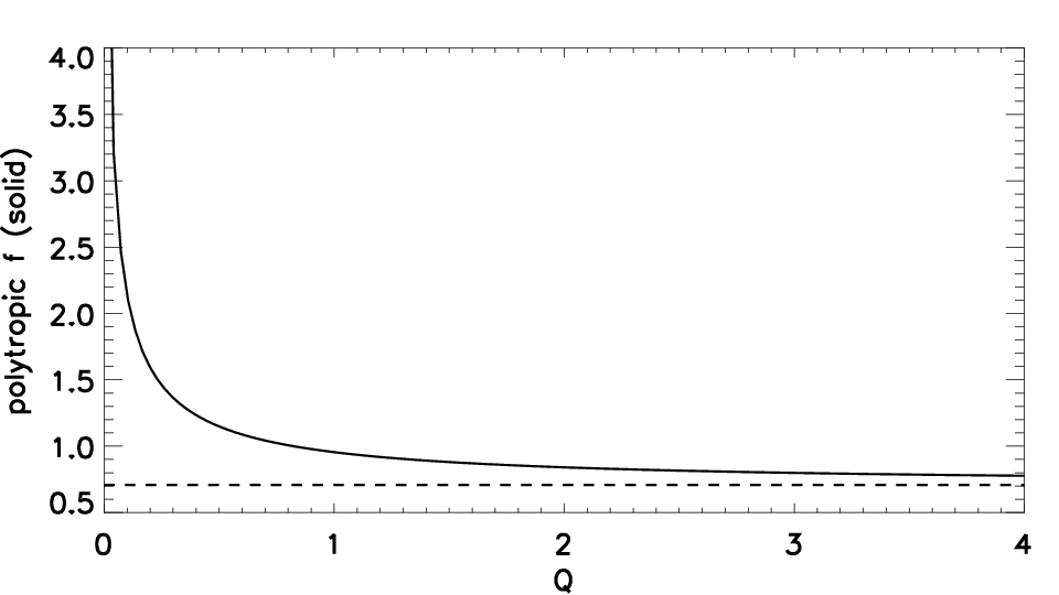
Given a fixed mid-plane temperature, the function is an inverse measure of the disk thickness, and increases with decreasing , as shown in Fig. 17. This corresponds to a thinner disk with increasing strength of vertical self-gravity.
Appendix B Relation between and the Toomre parameter
The Toomre parameter defined for razor-thin disks is
| (B1) |
where is the total column density. To relate our self-gravity parameter and , we replace by , and by , giving
| (B2) |
where each term on the right-hand-side is non-dimensionalized (see §III.2.1). Fig. 18 plots this relation for isothermal and polytropic disks.

Appendix C Reduction to linear hydrodynamics
Our task here is to remove the magnetic field and vertical velocity perturbations from the linearized equations. Let us first define operators
| (C1) |
and
| (C2) |
And we define the variables
| (C3) | ||||
| (C4) |
We first express the continuity equation in terms of horizontal velocity, density and potential perturbations. The vertical velocity perturbation is
| (C5) |
where the linearized momentum equation was used (i.e. eliminating between Eq. 19 and Eq. 20). Inserting this into the linearized continuity equation (Eq. 17), we obtain
| (C6) |
Next, we examine separately the cases of a vertical field with variable resistivity and that of a tilted field with uniform resistivity. (A similar procedure can be performed in the general case of a tilted field with variable resistivity.)
C.1. Vertical field with variable resistivity
First consider and in the linearized equations. Denoting the vertical derivative as (n), the equations of motion give
| (C7) | ||||
| (C8) |
for . Differentiating the divergence-free condition for the magnetic field gives
| (C9) |
We insert the expression for from Eq. C7 and the expression for from the component of the linearized induction equation (Eq. 23) to obtain
| (C10) |
Inserting the above expressions for , (Eq. C7) and (Eq. C10) into the right-hand-side of the -induction equation (Eq. 21 ) gives
| (C11) |
( has been assumed to obtain this.) We differentiate this expression with respect to and eliminate the resulting using Eq. C7, to obtain
| (C12) |
We follow a similar procedure as above to remove . We use Eq. C11 and Eq. C8 to eliminate and from the right-hand-side of the -induction equation (Eq. 22),
| (C13) |
We differentiate this expression with respect to , then eliminate and from the left-hand-side of the resulting expression using Eq. C13 and Eq. C8, respectively. We obtain
| (C14) |
C.2. Tilted field with uniform resistivity
Here we allow but take to be constant. We first obtain expressions for and . Differentiating the momentum equation and replacing the resulting using the divergence-free condition and using the momentum equation, we obtain an expression for which can be inserted into the induction equation. This gives
| (C15) |
We can insert this into the induction equation to obtain
| (C16) |
where we have also used the derivative of the momentum equation to eliminate . Recall , so that
| (C17) |
where the second equality results from the continuity equation.
Now consider
| (C18) |
where the first equality corresponds to the momentum equation and the second equality results from replacing using the induction equation. We can now use the above expressions for and (Eq. C15–C16) to obtain
| (C19) |
Similarly, we differentiate Eq. C16 and use the momentum equation to eliminate to obtain
| (C20) |
References
- [1] Abramowitz, M., & Stegun, I. A. 1965, Handbook of mathematical functions with formulas, graphs, and mathematical tables, ed. Abramowitz, M. & Stegun, I. A.
- [2] Aizenman, M., Smeyers, P., & Weigert, A. 1977, A&A, 58, 41
- [3] Armitage, P. J. 2011, ARA&A, 49, 195
- [4] Armitage, P. J., Livio, M., & Pringle, J. E. 2001, MNRAS, 324, 705
- [5] Balbus, S. A., & Hawley, J. F. 1991, ApJ, 376, 214
- [6] —. 1998, Reviews of Modern Physics, 70, 1
- [7] Balbus, S. A., & Papaloizou, J. C. B. 1999, ApJ, 521, 650
- [8] Bonanno, A., & Urpin, V. 2007, ApJ, 662, 851
- [9] Boss, A. P. 1997, Science, 276, 1836
- [10] —. 1998, ApJ, 503, 923
- [11] Chandrasekhar, S. 1961, Hydrodynamic and hydromagnetic stability, ed. Chandrasekhar, S.
- [12] Christodoulou, D. M. 1993, ApJ, 412, 696
- [13] Elmegreen, B. G. 1987, ApJ, 312, 626
- [14] Fan, Z., & Lou, Y.-Q. 1997, MNRAS, 291, 91
- [15] Fleming, T., & Stone, J. M. 2003, ApJ, 585, 908
- [16] Fromang, S. 2005, A&A, 441, 1
- [17] Fromang, S., Balbus, S. A., & De Villiers, J.-P. 2004a, ApJ, 616, 357
- [18] Fromang, S., Balbus, S. A., Terquem, C., & De Villiers, J.-P. 2004b, ApJ, 616, 364
- [19] Fromang, S., de Villiers, J. P., & Balbus, S. A. 2004c, Ap&SS, 292, 439
- [20] Fromang, S., Terquem, C., Balbus, S. A., & de Villiers, J.-P. 2004d, in Astronomical Society of the Pacific Conference Series, Vol. 321, Extrasolar Planets: Today and Tomorrow, ed. J. Beaulieu, A. Lecavelier Des Etangs, & C. Terquem, 262
- [21] Gammie, C. F. 1996a, ApJ, 457, 355
- [22] —. 1996b, ApJ, 462, 725
- [23] —. 2001, ApJ, 553, 174
- [24] Gammie, C. F., & Balbus, S. A. 1994, MNRAS, 270, 138
- [25] Goldreich, P., & Lynden-Bell, D. 1965a, MNRAS, 130, 97
- [26] —. 1965b, MNRAS, 130, 125
- [27] Goodman, J. 2003, MNRAS, 339, 937
- [28] Goodman, J., & Xu, G. 1994, ApJ, 432, 213
- [29] Gressel, O., Nelson, R. P., & Turner, N. J. 2012, MNRAS, 422, 1140
- [30] Helled, R., et al. 2013, ArXiv e-prints
- [31] Inutsuka, S.-i., Machida, M. N., & Matsumoto, T. 2010, ApJ, 718, L58
- [32] Jin, L. 1996, ApJ, 457, 798
- [33] Kim, J.-G., Kim, W.-T., Seo, Y. M., & Hong, S. S. 2012, ApJ, 761, 131
- [34] Kim, W.-T., & Ostriker, E. C. 2000, ApJ, 540, 372
- [35] —. 2001, ApJ, 559, 70
- [36] Kim, W.-T., Ostriker, E. C., & Stone, J. M. 2003, ApJ, 599, 1157
- [37] Kojima, Y., Miyama, S. M., & Kubotani, H. 1989, MNRAS, 238, 753
- [38] Landry, R., Dodson-Robinson, S. E., Turner, N. J., & Abram, G. 2013, ApJ, 771, 80
- [39] Lin, M.-K. 2012, ApJ, 754, 21
- [40] Lizano, S., Galli, D., Cai, M. J., & Adams, F. C. 2010, ApJ, 724, 1561
- [41] Lubow, S. H., & Martin, R. G. 2012, ApJ, 749, L37
- [42] Lynden-Bell, D., & Kalnajs, A. J. 1972, MNRAS, 157, 1
- [43] Mamatsashvili, G. R., & Rice, W. K. M. 2010, MNRAS, 406, 2050
- [44] Martin, R. G., Lubow, S. H., Livio, M., & Pringle, J. E. 2012a, MNRAS, 420, 3139
- [45] —. 2012b, MNRAS, 423, 2718
- [46] Menou, K., & Quataert, E. 2001, ApJ, 552, 204
- [47] Nakamura, T. 1983, Progress of Theoretical Physics, 70, 747
- [48] Ogilvie, G. I. 1998, MNRAS, 297, 291
- [49] Papaloizou, J. C., & Savonije, G. J. 1991, MNRAS, 248, 353
- [50] Papaloizou, J. C. B., & Lin, D. N. C. 1989, ApJ, 344, 645
- [51] Pessah, M. E., & Psaltis, D. 2005, ApJ, 628, 879
- [52] Reyes-Ruiz, M. 2001, ApJ, 547, 465
- [53] Sano, T., & Miyama, S. M. 1999, ApJ, 515, 776
- [54] Terquem, C. E. J. M. L. J. 2008, ApJ, 689, 532
- [55] Toomre, A. 1964, ApJ, 139, 1217
- [56] Turner, N. J., Fromang, S., Gammie, C., Klahr, H., Lesur, G., Wardle, M., & Bai, X.-N. 2014, ArXiv e-prints
- [57] Vorobyov, E. I. 2013, A&A, 552, A129
- [58] Yang, C.-C., Mac Low, M.-M., & Menou, K. 2012, ApJ, 748, 79
- [59] Zhu, Z., Hartmann, L., & Gammie, C. 2010a, ApJ, 713, 1143
- [60] Zhu, Z., Hartmann, L., Gammie, C. F., Book, L. G., Simon, J. B., & Engelhard, E. 2010b, ApJ, 713, 1134