Modeling interacting dynamic networks: II. Systematic study of the statistical properties of cross-links between two networks with preferred degrees

For the homogeneous population in the steady state, there is only one $\rho^{ss}(k)$, since all links are connected to nodes in the same network. Of all the distributions introduced above for two interacting networks, the most appropriate ones for this comparative study is the global distribution, $\rho_{1}^{ss}$, which should be same as $\rho_{2}^{ss}$ for this symmetric case. As we found, these quantities settle down quite rapidly, so that we were able to exploit the relatively large systems ($L=1000$ and $\kappa=250$) used in previous studies [1]. Starting with empty networks, we discard the first $1K$/$2K$ MCS for the single-/two-network model. Thereafter, we measure the quantities of interest every $100$ MCS and compile the average over $10^{4}$ measurements. The resultant $\rho^{ss}$’s are shown in Fig. 1. It is clear that there is no discernible difference between all three distributions, as might be expected.

For the reader’s convenience, we recapitulate known properties of $\rho^{ss}$ and how its form (neither Poisson nor Gaussian) can be understood [1]. We see that $\rho^{ss}\propto e^{-\mu\left|k-\kappa\right|}$ is a double exponential, i.e., a Laplacian. Our data indicate $\mu=1.08\pm 0.01$, which can be explained using a crude mean-field approximation to estimate the rates for our node to gain or lose a link. Respectively, these are $\Theta(\kappa-k)+1/2$ and $\Theta(k-\kappa)+1/2$, where $\Theta$ is the Heavyside function. The $\Theta$ terms correspond to how a chosen node will act, while the $1/2$ accounts for how its partner nodes will act. In the steady state, each node is ‘content’ on the average, and so, the probability to add/cut is just $1/2$. Balancing the gain/lose probability currents, we arrive at

which leads to $\rho^{ss}(k)\propto 3^{-\left|k-\kappa\right|}$, in excellent agreement with the data.

Needless to say, the same argument can be advanced for the symmetric two-network system, arriving at a similar result. However, as presented below, drastic differences between the single-network and the interacting networks emerge when we measure another quantity: $X$.

In a previous paper [1], we investigated this quantity briefly. In particular, we found that $X(t)$ displays very large fluctuations and, for systems with $L=1000$, it takes very long times ($\gg 3\times 10^{6}$ MCS) for $X$ to reach the limits of its range. To build reliable histograms, it would take even longer to collect enough data. Thus, we consider smaller systems for the remainder of this paper, namely, $L=100$ and $\kappa=25$. We also discard the initial $10^{7}$ MCS, to let the system reach steady state, before taking measurements every $100$ MCS for the next $2\times 10^{7}$ MCS. With the resultant time trace of $2\times 10^{5}$ points, we compile a histogram, which leads to $P^{ss}(X)$. We also construct a power spectrum. Specifically, we divide the entire time trace into 20 shorter ($10^{4}\equiv T$) ones and obtain Fourier transformations of each: $\tilde{X}(\omega)\equiv\sum_{t=1}^{T}{X(t)e^{i{\omega}t}}$ where $\omega=2{\pi}m/T~$($m{\in}[0,T-1]$). The power spectrum, $I(\omega)$, is defined as the average $\langle|\tilde{X}(\omega)^{2}|\rangle$ over these 20 FT’s.

The results are plotted (in red) in Figs. 2 and 3. The presence of a broad plateau in $P^{ss}(X)$ motivates us to explore the dynamics of ${X(t)}$, to see if it simply performs an unbiased random walk within the confines of two ‘soft walls.’ This conjecture is confirmed by the latter plot, in which we see that $I(\omega)$ indeed follows $1/\omega^{2}$ quite well, crossing over (for small $\omega$) to a constant dictated by the limits of $X$, namely, $0$ and $L^{2}$.

In stark contrast, the data displayed in green are indicative of very different behavior. Let us emphasize what $X$ is – in this homogeneous population of $200$ nodes, all preferring degree $25$. First, we randomly partition the system into 2 sets of 100 nodes, labelling one set ‘blue’ and the other ‘red.’ At any $t$, the total number of ‘red-blue’ links is defined as $X$. Clearly, if we focus on any one node, there can be up to 199 contacts, though $\kappa$ will limit the average to about $25.5$. Thanks to homogeneity and the randomness in the dynamics, we can expect half of these to be cross-links. Thus, we are not surprised by the peak of $P^{ss}(X)$ being located at $\sim 100\times 25.5/2=1275$. We can go further, to estimate the observed standard deviation ($\sigma_{X}\sim 25$) by the following crude argument. Denoting by $x$ the number of cross-links of any node, we already arrived at its mean, i.e., $\langle x\rangle=12.75$. If we assume that the distribution of $x$ is a binomial distribution (with probability 1/2 that the node acts on a cross-link), then this standard deviation is, roughly, $\sigma_{x}=\sqrt{25.5/4}$. Invoking the central limit theorem for 100 nodes, we easily find $\sigma_{X}=\sqrt{100}\sigma_{x}\simeq 25$, in excellent agreement with observation. As for its dynamics, we expect $X\left(t\right)$ to be governed by white noise, as confirmed by the green line in Fig. 3.

By contrast, $\sigma_{X}$ for the symmetric two-network system is over an order of magnitude larger: $\sim 300$! (Of course, by symmetry, the average $\left\langle X\right\rangle$ is expected to be the similar, i.e., $\sim 1250$.) The reason behind the failure of crude arguments for the symmetric, interacting two-network system is quite subtle. Exploring this non-trivial issue will be the topic of the third paper in the series [26]. There, we will study the opposite (indeed, extreme) limit of this system, thereby bringing the essence of this remarkable behavior into sharp focus. For the remainder of this paper, we will report on more systematic studies of $X$ in typical asymmetric two-network models.

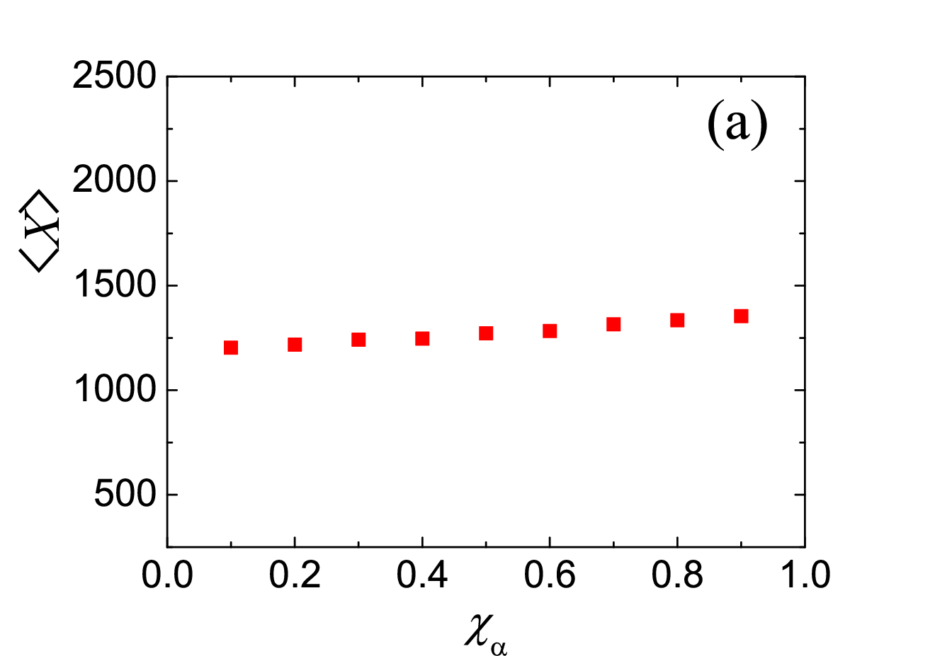
We begin by varying $\chi_{1}=\chi_{2}=\chi$, with $N_{\alpha}$ and $\kappa_{\alpha}$ kept at $100$ and $25$, respectively. Recall that $\chi$ controls effectively the interaction between two networks, since individuals with larger $\chi$ are more likely to take action on cross-links. Thus, $\chi=0$ represent two independent networks, while only cross-links are present in $\chi=1$ networks. For general $\chi$, however, it is not directly related to the value of $X$ (but only to the likelihood for $X$ to change). Therefore, our expectation is that changing $\chi$ would not affect $\langle X\rangle$ or $\sigma_{X}$. Fig. 4 shows the simulation results for $\chi=0.1,...,0.9$. Our expectation is largely borne out, especially for $\sigma_{X}$. There appears to be a slight rising trend in $\langle X\rangle$, $\sim 15\%$ over this entire range of $\chi$. It is difficult to explain these variations in detail, though the typical values deviate little from that in the symmetric case ($\chi=0.5;~~\langle X\rangle\sim 1272$), as predicted above. We will next see that more interesting behavior appears when we vary the other two control parameters.

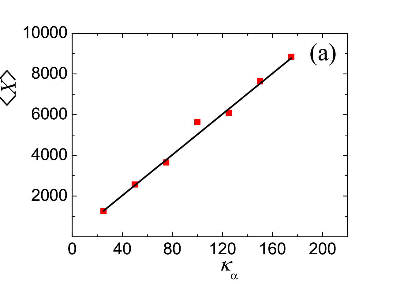
The next pair we vary is $\kappa_{1}=\kappa_{2}=\kappa$, with fixed $N_{\alpha}=L=100$ and $\chi_{\alpha}=\chi=0.5$. Fig. 5 shows the simulation results for $\kappa=25,50,75,...,175$. Needless to say, if $\kappa$ exceeds the total population size, ($200$ in simulations here), every link will be established quickly, and $X$ will be a constant $L^{2}=10^{4}$ and $\sigma_{X}\equiv 0$. Thus, our simulations sample essentially the entire range of meaningful $\kappa$’s here. Now, $\kappa$ controls the preferred degree of a node and so, it is not surprising that $\langle X\rangle\propto\kappa$. In particular, since $\rho_{\alpha}(k)$ is sharply peaked at $\kappa_{\alpha}$, a simple minded estimate is that each node has $\kappa_{\alpha}\chi_{\alpha}$ cross-links. Thus, we arrive at $\langle X\rangle\simeq\kappa_{\alpha}N_{\alpha}/2$ ($=50\kappa$ here), plotted as a solid line in Fig. 5 and in surprisingly good agreement with the data. We are unable to find a similar estimate for the behavior of $\sigma_{X}$. The most striking features there are: (i) $\sigma_{X}$ varies linearly with $\kappa$ and (ii) $\sigma_{X}$ is symmetric around its peaks at $100$. That $\sigma_{X}$ vanishes at both end points is clear, but it is unclear how other features arise. A phenomenological formula which accounts for these features is $\sigma_{X}\propto$ $\min\left(\langle X\rangle,L^{2}-\langle X\rangle\right)$, but how it emerges from the underlying dynamics is unknown. In stark contrast, since this system is also ‘symmetric,’ an argument similar to the above (for its counterpart in a homogeneous population) would provide $\sqrt{N\kappa/4}=\sqrt{25\kappa}$, which clearly fails to match the data. Understanding the properties of $\sigma_{X}$ here remains a challenge.

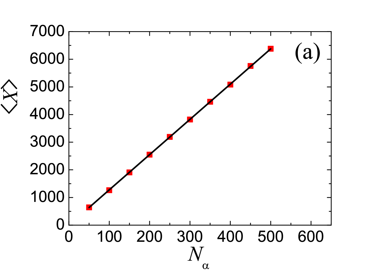
Finally, we vary $L=N_{1}=N_{2}$ while holding $\kappa_{\alpha}=\kappa=25$ and $\chi_{\alpha}=\chi=0.5$. Due to limited computing power, we only explored an order of magnitude around $100$: $L\in\left[50,500\right]$, the results of which are shown in Fig. 6. Again, the dependence of the mean, $\langle X\rangle$, is easy to understand, namely, $\kappa\chi L\simeq 12.5L$ (solid line). However, similar to the systems reported above, the behavior of $\sigma_{X}$ is more intriguing. In an inset of Fig. 6(b), we show a log-log plot of $\sigma_{X}$-$L$ and see that $\sigma_{X}$ scales well as $L^{0.63}$. Such anomalous scaling hints at critical phenomena and deserves a thorough investigation. In particular, the incidence matrix associated with the two communities can be viewed as an $L\times L$ Ising model (in the lattice gas language, with $0,1$ in the entries). Then, $X$ maps into $2M-L^{2}$, with $M$ being the total magnetization, while the variance $\sigma_{X}^{2}$ corresponds to the Ising susceptibility ($\times L^{2}$). So, our findings here imply a decreasing ‘susceptibility’ ($\sim L^{-0.74}$). This remarkable property can be argued qualitatively, as follow. Note that $\kappa\chi$ controls the creation of a cross-link, so that any particular link occurs, roughly, with probability $\kappa\chi/L$. Thus, increasing $L$ while holding $\kappa\chi$ fixed corresponds to an increasingly stronger magnetic field, which in turn, leads to a decreasing magnetic susceptibility. In the next paper of this series [26], such a mapping can be established analytically (for the two-population model with maximally opposite preferences), while a system with $N_{1}=N_{2}$ can be interpreted as a peculiar critical point [24].

In the previous subsection, we explored the region around a special symmetric two-network system by varying one pair of parameters (i.e., along certain lines). Here we turn our attention to a more general case, in which the networks differ by two parameters, specifically, just the sizes and the preferences. To make comparisons with the previously studied systems, we restrict ourselves to systems with fixed sums: $N_{1}+N_{2}=200$, $\kappa_{1}+\kappa_{2}=50$, and $\chi_{1}+\chi_{2}=1$. Moreover, from the results above (especially Fig. 4), we see that the effects of changing $\chi$ are minimal. Thus, we simply fix both $\chi$’s to $0.5$. As we vary $N_{\alpha}$, over the entire range, we need to keep, say, only $\kappa_{1}\leq\kappa_{2}$ to access the whole subspace of interest. This choice allows us to refer to $\alpha=1,2$ as the introverts and extroverts, respectively. In Fig. 7, we provide results for $\langle X\rangle$ and $\sigma_{X}$ as a function of $N_{2}$, for three different pairs of $\left(\kappa_{1},\kappa_{2}\right)$. We choose ($5,45$), ($15,35$), and ($25,25$) partly for convenience and partly for having $\kappa_{1}$’s ratios at $1:3:5$.

Focusing on the last pair first (blue points), we note that both curves are symmetric around $N_{2}=100$. Since the simulations were performed for pairs of $N_{2}$ around 100, the observed symmetry is an indication of the level of our statistical errors. The values of $\langle X\rangle$ and $\sigma_{X}$ at the center are entirely consistent with the findings shown above: approximately $1300$ and $300$ respectively. Away from the center, $\langle X\rangle$ appears to decrease slowly at first, but turns up when $N_{2}$ reaches to $\sim 10\%$ of the boundaries. The slow decrease is related to $N_{1}N_{2}=\left(200-N_{2}\right)N_{2}$, the maximum allowed value for $X$. Indeed, in this regime, the fraction

hovers around 13%, i.e., $\sim\kappa\chi$ divided by the average number of nodes in each community. On the other hand, the non-monotonic behavior can hardly be expected. In the next subsection, we will present an approximation scheme which can provide some insight into this remarkable phenomenon.

Turning to the two asymmetric cases, we are not surprised by the lack of symmetry in the curves. However, there are prominent and interesting features, the origins of which do not readily come to mind. First, the levels of $\langle X\rangle$ are generally reduced, despite both $\chi$’s being held at 0.5 and the average preference remaining at 25. Specifically, for a wide range of $N_{2}\gtrsim 100$, the $f$’s are relatively constant, matching roughly the ratio $1:3:5$. Thus, it appears that the introverts are controlling the level of cross-links. Why the extroverts play a lesser role may be argued as follows: When the number of extroverts is well above $\kappa_{2}$, they can be ‘content’ by maintaining more links to other extroverts, instead of adding cross-links. Of course, it would be highly desirable to formulate an analytic and more convincing approximation scheme. Second, in addition to the sharp upturn for $N_{2}\sim 200$, the peaks of $\langle X\rangle$ are shifted to smaller $N_{2}$, to approximately $20$ and $50$ for $\kappa_{1}=5$ and $15$ respectively. These features can also be roughly argued. Given that the preferred degrees are generally less than the number of nodes, it is understandable that the introverts are more likely to be frustrated, by the eagerness of extroverts to make cross-links. As we decrease $N_{2}$, (especially to values below $N_{1}$) we can expect such frustration to decrease, leading to the rise in $\langle X\rangle$ observed. Arguably, an ‘optimal’ state might be characterized by a balance between the total number of cross-links the introverts prefer, $N_{1}\kappa_{1}$, and that of the extroverts, $N_{2}\kappa_{2}$. (Note that we can ignore $\chi$ for this rough argument, since it affects predominantly the rate of actions on cross-links). This balance occurs at $N_{2}=4\kappa_{1}$ for our parameters, i.e., $20$ and $60$ for the runs with black and red points, respectively. While such arguments produce a rough understanding of the data, more quantitative improvements are clearly needed.

Lastly, we turn to the fluctuations in the cross-links, characterized here by only the standard deviation $\sigma_{X}$, see Fig. 7(b). As pointed out above, these are far larger than naively expected and explaining their presence remains a challenge. Here, we merely highlight what is in the figure: the asymmetric curves for $\kappa_{1}\neq\kappa_{2}$, the variation by over an order of magnitude, and the ‘calming influence of the more introverted.’ The last of these comments refers to the almost constant $\sigma_{X}$ for the $\kappa_{1}=5$ case. We end this subsection with another observation. Noting that the peaks of $\sigma_{X}$ for the asymmetric $\kappa$’s are also displaced toward the peaks of $\left\langle X\right\rangle$, we plot a ‘normalized standard deviation,’ $\sigma_{X}/\left\langle X\right\rangle$, see inset in Fig. 7(b). It is interesting that the peaks here are now located much closer to the center (though the curves remain asymmetric). Perhaps a detailed analysis of this quantity will facilitate the formulation of a viable theory.

In this last subsection, we present an approximation scheme which provides reasonably good agreement with data in a special regime. It is clear that, in a typical point in parameter space, there are so many competing features in our model that the contributions of all these factors will be difficult to untangle. A remarkable phenomenon – the upturn of $\left\langle X\right\rangle$ as $N_{2}$ nears its upper bound in Fig. 7(a) – is observed. Moreover, it appears that $\left\langle X\right\rangle$ assumes the same value at $N_{2}=190$ for all three pairs of $\kappa$’s! It behooves us, therefore, to explore this regime in more detail. The result, shown in Fig. 8, hints at the existence of some underlying ‘universal’ properties. Focusing on this regime, we discover that a simplification emerges, allowing us to gain some insight into this universality.

In the regime of interest, introverts are seriously outnumbered and highly frustrated. In other words, they find themselves with far more contacts than they prefer (i.e., $k\gg\kappa_{1}$), so that, when selected to act, they will always cut a link. A more precise and general characterization of this regime is $N_{1}\kappa_{1}\chi_{1}\ll N_{2}\kappa_{2}\chi_{2}$. The result of this activity is that there are no (or extremely few) $I$-$I$ links in the system, so that we can attempt an approximation scheme for $\rho_{1}^{ss}\left(k\right)$, the degree distribution of an $I$.²² 2 Note that, since we have assumed $k_{11}=0$, we can drop the subscripts in $k_{12}$, while $\rho_{12}\left(k\right)$ is also identical to $\rho_{1}\left(k\right)$. From $\rho_{1}^{ss}$, the average $\left\langle k\right\rangle$ can be computed. Since every link is a cross-link, $\left\langle X\right\rangle$ is just $N_{1}\left\langle k\right\rangle$.

The strategy here is the same as the one used for the single network: finding the steady state $\rho^{ss}$ by balancing the rates for increasing and decreasing $k$, namely,

where $W[k\rightarrow k^{\prime}]$ specifies the probability for a node with degree $k$ to become $k^{\prime}$. To find the appropriate $W$’s here, we rely on the following argument. Focus on a particular introvert, $i$, with existing degree $k$. For the regime of interest, we can assume $k>\kappa_{1}$, so that the only way for it to gain a link is for an extrovert (not already connected to $i$) choosing to add a cross-link to it. Several factors contribute to the rate for such a process:

• •

  $\left(N_{2}-k\right)/N$, the probability for an extrovert not connected to $i$ to be selected

• •

  $w_{2}^{+}$, the probability that this extrovert will add a link

• •

  $\chi_{2}$, the probability for it to add a cross-link ($1/2$ here), and

• •

  $p$, the probability that this cross-link is added to $i$.

Now, in this regime, we believe the extroverts should be mostly ‘content’ ($\kappa_{2}\ll N$). This belief is supported by the observed degree distributions, a typical case shown as red points in Fig. 9(a). Thus, we will approximate $w_{2}^{+}$ by $1/2$. As for the last quantity, $p^{-1}$ should be the number of introverts unconnected to our extrovert. We may estimate it by $N_{1}\left(1-f\right)$, where $f$ is the fraction of cross-links that are present. To be slightly more accurate, especially crucial for small $N_{1}$, we recognize that our extrovert is already connected to $i$ and so, we propose

Putting the factors together, we have

On the other hand, the contributions to $W[k+1\rightarrow k]$ come from two processes. One is node $i$ being selected to cut a cross-link. The probability of selecting this particular node $i$ is $1/N$, and with rate $1$ it will cut a link. But this action will be taken on a cross-link only with probability $\chi_{1}$ ($1/2$ here). In the other process, an extrovert connected to $i$ is chosen (probability $k/N$) and cuts one of its cross-links (probability $w_{2}^{-}\chi_{2}\simeq 1/4$). Following the argument above for $p^{-1}$, we have

Of course, here $p$ corresponds to the probability that the extrovert cuts the cross-link to $i$. Therefore, we reach at

With explicit expressions for the $W$’s, we exploit Eqn. (7) to derive a recursion relation for the steady state degree distribution:

where

Thus, $\rho_{1}^{ss}\left(k\right)$ is explicitly

where $\rho_{1}^{ss}\left(0\right)$ can be fixed by the normalization $\Sigma_{0}^{N_{2}}\rho_{1}^{ss}\left(k\right)=1$.

So far, $f$ is not a known quantity. But it can determined self consistently, through the equations

The result is a prediction (i.e., no fitting parameters) for $\rho_{1}^{ss}$ and so, $\left\langle X\right\rangle$. Plotted as black lines in Figs. 9 and 8, these predictions agree remarkably well – provided we remain in the $N_{1}\ll N_{2}$ regime. Clearly, the deviations of $\left\langle X\right\rangle$ from the theoretical curve in Fig. 8 reflect the limits of this regime.

Finally, we return the issue of ‘universality.’ Note that results Eqns. (13,14,15) are independent of the $\kappa$’s. Of course, their validity relies on the assumption that $\left\langle k_{1}\right\rangle\gg\kappa_{1}$, which seems reasonable in these cases where all the introverts are highly frustrated. In Figs. 9(b), we show data for a more extreme system ($N_{1},N_{2}=5,195$) in which this notion of universality is indeed well borne out. An alternative perspective is that, in this regime, the $N_{1}\times N_{1}$ block of the full $N\times N$ adjacency matrix is frozen at zero, so that much of what we wish to compute can be gleaned from the smaller $N_{1}\times N_{2}$ incidence matrix. As long as we restrict ourselves to considering ‘zero $N_{1}\times N_{1}$ blocks,’ the role of $\kappa_{1}$ is entirely marginal.

References

- [1] Liu W, Jolad S, Schmittmann B and Zia R K P 2013 J. Stat. Mech. Theory Exp. 2013 P08001
- [2] Strogatz S H 2001 Nature 410 268
- [3] Albert R and Barabási A-L 2002 Rev. Mod. Phys. 74 47
- [4] Dorogovtsev S N and Mendes J F F 2002 Adv. Phys. 51 1079
- [5] Newman M E J 2003 SIAM Rev. 45 167
- [6] Estrada E, Fox M, Higham D and Oppo G-L (eds) 2010 Network Science: Complexity in Nature and Technology (Springer, New York)
- [7] Watts D J and Strogatz S H 1998 Nature (London) 393 440
- [8] Albert R, Jeong H and Barabási A-L 1999 Nature (London) 401 130
- [9] Barabási A-L and Albert R 1999 Science 286 509
- [10] Barrat A, Barthelemy M and Vespignani A 2008 Dynamical processes on complex networks (Cambridge University Press)
- [11] Dorogovtsev S N, Goltsev A V and Mendes J F F 2008 Rev. Mod. Phys. 80 1275
- [12] Gross T, D’Lima C J D and Blasius B 2006 Phys. Rev. Lett. 96 208701
- [13] Gross T and Blasius B 2008 J. R. Soc. Interface 5 259
- [14] Rinaldi S, Peerenboom J and Kelly T 2001 IEEE Contr. Syst. Mag. 21 11
- [15] Panzieri S and Setola R 2008 Int. J. Model. Ident. Contr. 3 69
- [16] Vespignani A 2010 Nature (London) 464 984
- [17] Buldyrev S V, Parshani R, Paul G, Stanley H E and Havlin S 2010 Nature (London) 464 1025
- [18] Buldyrev S V, Shere N W and Cwilich G A 2011 Phys. Rev. E 83 016112
- [19] Kurant M and Thiran P 2006 Phys. Rev. Lett. 96 138701
- [20] Erdős P and Rényi A 1959 Pub. Math. 6 290
- [21] Platini T and Zia R K P 2010 J. Stat. Mech. Theory Exp. 2010 P10018
- [22] Zia R K P, Liu W, Jolad S and Schmittmann B 2011 Physics Procedia 15 102
- [23] Jolad S, Liu W, Schmittmann B and Zia R K P 2012 PLoS ONE 7(11) e48686
- [24] Liu W, Schmittmann B and Zia R K P 2012 EPL 100 66007
- [25] Zia R K P and Schmittmann B 2007 J. Stat. Mech. Theory Exp. 2007 P07012
- [26] Liu W, Bassler K E, Schmittmann B, and Zia R K P to be published.