Spin and impurity effects on flux-periodic oscillations in core-shell nanowires
Abstract
We study the quantum mechanical states of electrons situated on a cylindrical surface of finite axial length to model a semiconductor core-shell nanowire. We calculate the conductance in the presence of a longitudinal magnetic field by weakly coupling the cylinder to semi-infinite leads. Spin effects are accounted for through Zeeman coupling and Rashba spin-orbit interaction (SOI). Emphasis is on manifestations of flux-periodic (FP) oscillations and we show how factors such as impurities, contact geometry and spin affect them. Oscillations survive and remain periodic in the presence of impurities, noncircular contacts and SOI, while Zeeman splitting results in aperiodicity, beating patterns and additional background fluctuations. Our results are in qualitative agreement with recent magnetotransport experiments performed on GaAs/InAs core-shell nanowires. Lastly, we propose methods of data analysis for detecting the presence of Rashba SOI in core-shell systems and for estimating the electron g-factor in the shell.
pacs
73.63.Nm, 71.70.Ej, 73.22.DjI Introduction
Recent years have seen significant progress in the development and fabrication of semiconductor nanostructures. Nanowires of diameters of the order of nm can now be grown.[1, 2, 3, 4] Core-shell nanowires are composed of a thin layer (shell) surrounding a core in a tubular geometry. The cross section may be circular, but also polygonal (e. g. hexagonal) reflecting the lattice structure of the materials. If both shell and core are semiconductors, they may be chosen such that the difference in conduction band energies forms a potential barrier confining carriers to either the core[5, 6] or the shell.[7, 8] Recent examples include nanowires composed of an InAs shell grown on a GaAs core resulting in the formation of a conductive electron gas in the shell which may be further augmented by modulation doping the core.[9, 10] Such systems provide a fascinating means for studying fundamental quantum effects such as interference.
A prominent interference phenomenon due to the interaction of electromagnetic potentials with charged particles is the Aharonov-Bohm effect,[11] which arises because wave functions that enclose a magnetic flux acquire a flux-dependent phase shift. Furthermore, the corresponding energy levels are periodic in the flux[12] and FP oscillations have indeed been observed for example in the resistance[13] and magnetization[14] of rings pierced by a magnetic flux. A couple of theoretical papers have addressed FP oscillations in core-shell systems and found that spin ruins the periodicity due to Zeeman splitting. In Ref. 15 the magnetization of closed shells was analyzed and the robustness of FP oscillations to a nonzero shell thickness demonstrated. Additionally, it was shown that while static donor impurities affect the shape and phase of magnetization oscillations strongly, electron-electron interaction tends to weaken their effects on the oscillations. Magnetoconductance oscillations in cylindrical quasi-one-dimensional shells were treated in Ref. 16 and FP oscillations predicted assuming a narrow surface confinement. Later, magnetoresistance measurements on core-shell nanowires revealed the existence of FP oscillations,[8] which were recently shown to manifest because transport is mediated by closed-loop angular momentum states encircling the core, tying the oscillations to the spectrum.[9]
In this paper, we analyze the energy spectrum, charge and current densities of electrons confined to a closed cylindrical surface of finite length pierced by a longitudinal magnetic flux. We calculate the magnetoconductance of the finite system by coupling it to leads. In particular, we focus on FP oscillations in both conductance and spectrum and discuss the effects of core donor impurities and electron spin, which is included through Zeeman splitting and Rashba SOI and may thus affect transport nontrivially. The experimentally-relevant effects of nonuniform coupling to leads are also discussed. While donor impurities dampen conductance oscillations, they remain resolvable after extensive averaging over multiple random impurity configurations, assuming realistic donor densities. Using parameters comparable to those reported in Ref. 9, we attribute background conductance oscillations, which are superimposed on the FP oscillations, to an interplay between the finite system length and Zeeman splitting, propose means for detecting the presence of Rashba SOI and discuss a method for estimating the shell electron g-factor based on transport data.
II Quantum mechanical model for core-shell nanowires
We consider a cylindrical core-shell nanowire of radius and length where the shell and core are composed of different semiconductors such that the difference in conduction band energies confines conduction electrons to the shell with negligible wavefunction leakage into the core. We assume that the shell thickness is small compared to and such that only the lowest radial mode is occupied and approximate the shell as infinitely thin. In principle corresponds to the mean radius of the shell and thus we model the nanowire as a two-dimensional cylindrical surface.
II.1 Closed wire
The starting point for a quantum mechanical model of electrons confined to a cylindrical surface of finite length, described by the cylindrical coordinates , is the single-electron Hamiltonian. In the presence of a longitudinal magnetic field with vector potential , the kinetic momentum yields the kinetic energy term
| (1) |
Here, is the effective mass of shell conduction electrons, the longitudinal magnetic flux piercing the cylinder and the magnetic flux quantum. To model finite cylinder length we use hard-wall potentials at the cylinder edges,
| (2) |
The electron spin yields a Zeeman term which in a longitudinal field has the form
| (3) |
where is the free electron mass, the effective g-factor of shell conduction electrons and the cyclotron frequency. In addition, we model Rashba SOI in core-shell geometries as arising due to interactions between the shell electron gas and ionized donors in the core, producing an approximately radial electric field. For our model it reads[17, 18, 19]
| (4) |
where determines the SOI strength and describes the tangential spin projection. A Dresselhaus type SOI, arising due to inversion asymmetry in the crystal structure of the shell, may also be included. Such effects are typically minor in InAs compared to those of the Rashba term, and we have therefore chosen to neglect them in the present context.
The total single-electron Hamiltonian of the closed central system is the sum of the terms in Eqs. (1) to (4),
| (5) |
Electron-electron interaction is neglected. We solve numerically the time-independent Schrödinger equation
| (6) |
in the basis corresponding to eigenstates of the first three terms in
| (7) |
Here is the orbital angular momentum quantum number, describes the spin projection along , are eigenspinors of and arises due to the longitudinal quantization.
We calculate the charge and current density for a shell conduction electron in the state as[20]
| (8) |
where the integral extends over the cylinder surface. At vanishing temperature K, placing electrons in the system will fill up the energetically lowest states and the total densities and are obtained by summing up their contributions. The current density operator is
| (9) |
where H.c. denotes the Hermitian conjugate, is the coordinate at which the density is evaluated and the electron coordinate. The velocity operator is determined by solving the Heisenberg equation of motion, using from Eq. (5):
| (10) |
II.2 Transport formalism
In order to calculate the conductance of the finite cylindrical system we couple it to leads. The leads are taken as cylindrical continuations of the finite central system with the same radius , extending from the junctions to the left (L) and right (R) along the -axis over and , respectively. Their purpose is to supply phase-coherent electrons to the now open central system (S) from two reservoirs (or contacts) maintained at chemical potentials and .[21] Electrons propagate through the leads to the junctions where, as with the central system, hard-wall boundary conditions are imposed, but injections into the central system are made possible through a geometry-dependent coupling kernel in the form of an overlap integral between each lead and the central cylinder.[22] Aside from backscattering due to hard-wall boundary conditions, we assume that all scattering takes place in the central system. Since in Eq. (5) is time-independent, only elastic scattering is considered.
We define the Hamiltonians and eigenstates of the isolated left () and right () lead, respectively. The left and right leads are coupled to the central system by assuming coupling terms and , respectively, at each junction. The two leads are mutually coupled only indirectly through the central system. The time-independent Schrödinger equation of the entire coupled system is written in the matrix form[23, 24, 25]
| (11) |
where is the projected ket onto region . By solving for and in the first and third equations, the retarded Green’s operator of the central system follows from the second equation[26, 27, 28]
| (12) |
where leads enter through the energy-dependent self-energy operators
| (13) |
for the left and right leads. Note that acts on the central system subspace. Here, and are the retarded Green’s operators of the isolated leads
| (14) |
where and . The self-energy operators are generally not hermitian. Their appearance in motivates the consideration of an effective central system Hamiltonian which is clearly not hermitian and thus has a complex spectrum. Provided the self-energies can be regarded as “small” terms compared to , the spectrum of will correspond to the slightly-shifted spectrum of with added imaginary parts which provides level-broadening in the central system.[21, 24]
The current through the central system from right lead to left lead is given by the (spin-resolved) Landauer formula[21, 23, 25, 28]
| (15) |
where is the Fermi-Dirac distribution function of lead . The operators are defined as (,)
| (16) |
Assuming that and where the bias , at low temperatures the current becomes linear in yielding the conductance of the coupled central system in the linear-response regime[21, 23, 26]
| (17) |
which will be used to calculate conductance in this paper. Energy-dependent quantities are evaluated at the chemical potential which is uniform throughout the system. From Eq. (12) it is clear that and hence are primarily determined by the geometry and properties of the central system through . The leads enter through the self-energies and provide level-broadening for the central system as discussed before.
In order to evaluate the trace in Eq. (17), we construct the necessary operators in the basis of central system eigenstates in which is diagonal. Specifically, we construct the matrix representation of at a given energy with matrix elements
| (18) |
and invert it numerically. Evaluating the self-energy matrix elements with also yields the matrix representations of in Eq. (16) and is thus sufficient to calculate using Eq. (17).
The matrix elements are calculated by inserting closure relations for lead and defining a coupling kernel between the lead in question and the central system. To illustrate this procedure, let us consider the left lead matrix element . The normalized eigenstates of the isolated left lead constitute an orthonormal basis for the state space of the isolated left lead and thus satisfy a closure relation there. Here, is the set of all necessary orbital and spin quantum numbers. In this basis, given in Eq. (14) is diagonal and can be written as
| (19) |
The coupling Hamiltonian thus enters as an overlap matrix element between the left lead and the central system eigenstates. Using a coordinate closure relation for the entire coupled system the overlap matrix element becomes
| (20) |
where the integrals extend over the central system () and both leads (,). The functions and are localized in the central system and left lead respectively and vanish everywhere else, so the two space integrals reduce to integrals over the left lead () and central system (). They couple through
| (21) |
which we define as the coupling kernel between the left lead and the central system. The overlap matrix element thus becomes
| (22) |
which can be evaluated with a suitable choice of provided the eigenstates and are known. For lead we use
| (23) |
where and are coordinates of the central cylinder and lead , respectively. The kernel is real and due to the -function conserves the angular coordinate between lead and central system producing a circularly symmetric coupling. is a parameter with the dimension energy/length which governs the overall strength of the coupling and can be used to control level-broadening in the central system. The parameter determines how rapidly the coupling decreases along the cylinder axis. To be consistent with the assumption of only indirect coupling between leads via the central system, is chosen such that the exponential coupling of a given lead vanishes in the vicinity of the other lead. The -modulated overlap integral in Eq. (22) incorporates the geometry and properties of both central system and leads giving state-dependent level-broadening.
The eigenstates of the leads are used to calculate . We include the magnetic flux in the leads and let it couple to electron spin through the Zeeman term. Hence, the Hamiltonians and of the left and right leads both have the form of Eqs. (1) plus (3) with imposed hard-wall boundary conditions at the junctions. The eigenstates of the isolated leads are thus characterized by three quantum numbers , . For the left lead
| (24) |
where , , and is an eigenspinor of . Right lead states are obtained by switching the index and setting such that they vanish at .
Using the eigenstates of [Eq. (5)] and the isolated leads [Eq. (24)] along with the kernel of Eq. (22), the self-energy matrix elements [Eq. (19)] are evaluated. Note that each self-energy matrix element contains two overlap integrals. The sum over the lead quantum number is truncated at the same value as the central system angular modes [Eq. ()]. For each , both spin projections are included and the integral over the continuous lead quantum number is done analytically by extension into the complex plane. From the self-energy matrix elements of both leads at , the matrix representations of the operators [Eq. (12)] and [Eq. (16)] follow and then is calculated using Eq. (17).
III Transport calculations
III.1 Model parameters
We consider a cylindrical shell using material parameters for InAs.[18, 30] The effective electron g-factor is and we use the Rashba SOI parameter meVnm which corresponds to a strong confining radial field. As the effective mass of conduction electrons at the -point we use . The dielectric constant is taken as . Unless otherwise specified, we assume a shell radius nm and nanowire length nm corresponding to an aspect ratio which ensures that angular and axial quantization result in approximately equal level spacing. Growth of nanowires of comparable radius has been reported in Refs. 8, 31, 1.
In the following subsections we discuss FP oscillations and spin effects on the magnetoconductance in our model. We furthermore consider cylindrical symmetry breaking due to Coulomb impurities and a broken circular symmetry of the coupling scheme.
III.2 Flux-periodic oscillations
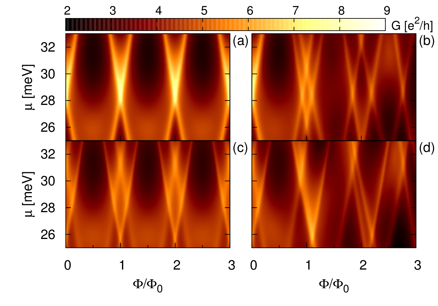

Figure 2 shows the calculated conductance of a finite cylinder as a function of and . Different subfigures demonstrate the effects of the spin-dependent terms Eqs. (3) and (4) on . For reference, the flux-dependence of the closed cylinder spectrum is given over the corresponding energy range in Fig. 2. A detailed analysis of the spectra of closed cylinders of different aspect ratios is given in Ref. 15.
Roughly, conductance peaks correspond to intersections with the spectrum, so manifests as the broadened and slightly shifted spectrum of . This is due to the self-energy operators of the leads in [Eq. (12)]. We have deliberately chosen coupling parameters such that the induced shift and level-broadening are both of the order meV, such that the close correspondence between spectrum and conductance in Figs. 2 and 2 becomes evident. Our intention is thus to minimize the effects of the leads and the particular form of the coupling kernel [Eq. ()] on , which should be governed by the physics of the central system, i. e. by .
In the absence of Rashba SOI, the central system Hamiltonian has the eigenstates Eq. (7). At each level is quadruply degenerate, except states with which are only doubly degenerate. At states with successively higher orbital angular momentum pile into a given axial mode forming a ring-like spectrum until a new axial mode sets in. Hence, the spectrum can be thought of as a superposition of the ring-like spectra of different axial modes. When the spectrum is periodic in with period , i. e. increasing by is equivalent to reducing by at a fixed energy.[32] Hence, the oscillations are similar to Aharonov-Bohm oscillations which have been studied extensively in ring-like [20, 33, 34, 35, 36, 37, 38, 39, 40, 41] and cylinder-like [42, 8, 15, 16, 43] geometries, i. e. without and with a longitudinal degree of freedom, respectively. There is no coupling between and longitudinal electron motion, so FP oscillations on cylinders manifest due to the same principles as those observed in quantum rings, but with an added degree of freedom through the length-dependent -term.
III.3 Zeeman spin effects
Including the Zeeman term adds the -linear term to the spectrum such that the energy of spin down (up) states increases (decreases) with increasing . Hence spin-degeneracy is lifted as a comparison between Figs. 2 (a) and (b) shows. This effect is pronounced in InAs due to the large value of and ruins the periodicity of the spectrum.[15, 16]

Figure 3 shows the equilibrium current density [Eq. (8)] on the surface of the cylinder uncoupled to leads at with . The current density is obtained by summing up the contributions from the lowest states, a realistic number of electrons given the density reported in Ref. 18. Setting does not change in this case, since the Zeeman term does not affect the velocity operator [Eq. (10)]. However, spin-splitting increases with , changing the orbital characteristics of the energetically lowest states as they become spin-polarized, which affects . The system is invariant under rotations around the -axis since where is the rotation operator around the cylinder axis by the finite angle . As a result, the electron density on the cylinder surface is circularly symmetric. Since the velocity operator commutes with , is rotationally invariant and because is purely imaginary for all , the axial component vanishes [Eqs. (7) and (9)]. Thus is composed of concentric circles, each of constant current density. In the closed system, and thus reflect that electrons enclose a magnetic flux resulting in the FP oscillations observed in the spectrum.
In Figs. 2 (a) and (b) we show the calculated conductance of a cylinder coupled to leads as a function of and without (a) and with (b) the Zeeman term. The flux-dependence of the spectrum in the corresponding energy range is given in Figs. 2 (a) and (b). When the conductance evidently retains the periodicity of the spectrum and hence exhibits oscillations with period . While the conductance oscillations are periodic for all values of , their phase and shape in a single period is sensitive to the value of considered. Including the Zeeman term breaks the periodicity of conductance oscillations as it does to the spectrum.[16] The resulting spin-splitting of states can produce magnetoconductance curves which are gradually increasing, decreasing or relatively stable at low values of depending on the value of considered, as may be seen in Fig. 2 (b). This point will be further discussed in Sec. V. Our numerical results show the same overall trends in the density of states (DOS) depending on as the flux is varied.
III.4 SOI effects
Including Rashba SOI, we obtain the eigenstates of given by Eq. (5) by numerical diagonalization in the basis (7). Examples of the resulting energy spectrum are shown in Figs. 2 (c) and (d) for and , respectively. Compared to the spectrum with and in Fig. 2 (a) the Rashba term generally lifts spin-degeneracy at , but crossings still appear at integer values of due to the fact that commutes with .
Interestingly, despite Rashba SOI introducing the flux-linear term into the Hamiltonian, the spectrum remains periodic in . Unlike the Zeeman term, the Rashba term alone does not break the periodicity of oscillations.[16] Since does not couple to in , we can look for an explanation by considering a quantum ring limit . This results in vanishing longitudinal electron motion so and the term vanishes from the Hamiltonian. The ring-limit spectrum with is
| (25) |
which is indeed periodic in with period . Since the ring-limit and the finite-cylinder spectra couple identically to , it follows that the spectrum of a finite cylinder with Rashba SOI alone is periodic in in agreement with our numerically obtained spectrum Fig. 2 (c). Provided , the flux-dependence of the spectrum is qualitatively similar with and without Rashba SOI aside from the splitting of degenerate states [Figs. 2 (a) and (c)]. We emphasize that the ring-limit spectrum with Rashba SOI [Eq. (25)] differs from known results for quantum rings. The reason is that in cylindrical core-shell geometries the confining electric field is radial,[18, 16] whereas in quantum rings it is typically assumed to be perpendicular to the ring, i. e. along the direction.[44, 20, 36, 39, 45]
While the Rashba term Eq. (4) does not commute with or , it does commute with and hence with the rotation operator , which means that the Rashba term does not break the circular symmetry of the system. As a result, the charge and current densities at a fixed -coordinate remain uniform around the circumference of the cylinder when Rashba SOI is included. In fact, when the resulting equilibrium current density of electrons is almost indistinguishable from that given in Fig. 3 where , despite the presence of SOI-dependent terms in both and [Eq. (10)]. In particular, still vanishes which suggests that the densities of the observables and vanish everywhere. Our numerical results show that this is indeed the case. This is contrary to what happens on an infinitely long cylinder, where Rashba SOI alone has been shown to produce a nonvanishing tangential spin density .[18] To understand the difference, let us consider an infinitely long cylinder . As is shown in Appendix A, the normalized eigenspinors of an infinitely long cylinder with Rashba SOI but can be written as
| (26) |
with degenerate energies . The coefficients can be chosen such that they satisfy and , where is purely imaginary and purely real. From this, it indeed follows that in agreement with Ref. 18. There is however a fundamental difference between eigenstates on the finite and infinite cylinders, namely that always vanishes on the former, but not on the latter except if . On the finite cylinder with , because the spectrum of is nondegenerate at arbitrary values of and , where is the spatial inversion operator over the cylinder center. Hence, the eigenstates have definite parity relative to the cylinder center[46] and so always since only couples states of opposite parity. This difference alone implies nonzero on the infinite cylinder and invalidates a direct comparison between the infinite and finite systems. But since one can easily construct infinite-cylinder eigenstates that satisfy and are thus physically the “closest” ones to finite-cylinder eigenstates. The most general form satisfying is
| (27) |
where . Analogous to the finite cylinder, one then obtains vanishing tangential spin density which reconciles the two cases.
Figure 2 (c) shows the conductance of the finite cylinder coupled to leads with Rashba SOI included and . Compared with the case shown in Fig. 2 (a), the Rashba term causes a split and shift of conductance curves. Generally, this results in the appearance of more peaks of smaller amplitude within a given period at fixed . The splitting and shift is analogous to that which occurs in the closed-cylinder spectrum [Figs. 2 (a) and (c)], further demonstrating the close correspondence between spectrum and conductance in this formalism. As with the spectrum, including Rashba SOI alone is insufficient to break the periodic oscillations in conductance with at a fixed .[16] Instead, it modifies the shape and phase of conduction curves within a single period. Including the Zeeman term also breaks the periodicity of the spectrum as in the case when , see Fig. 2 (d). Again, this is reflected in the conductance as Fig. 2 (d) shows.
III.5 Broken circular symmetry of the contacts

From an experimental point of view, the assumption of a circularly symmetric coupling kernel [Eq. (23)] may be unrealistic, as contacts typically only connect to restricted parts of the wire.[9, 10, 8] To check whether the FP conductance oscillations are sensitive to this circular symmetry, we break it explicitly by restricting the coupling regions to finite angles. Assuming vanishing coupling at junction except in the angular interval , we introduce step functions into the coupling kernel in Eq. (23)
| (28) |
Figure 4 compares the magnetoconductance of the cylinder with restricted and unrestricted coupling. Spin is neglected for simplicity. We see that the oscillations indeed remain flux-periodic. However, the overall conductance is reduced and the shape of the oscillations within a given period may change significantly depending on the intervals considered.
IV Effects of impurities in the core
In realistic core-shell nanowires the number of shell conduction electrons may be increased by modulation doping the core with donors.[10, 9] This produces ionized Coulomb impurities in the core, i. e. attractive potentials to shell conduction electrons. In this section we discuss the effects of such donor-like impurities on both closed and open cylindrical systems.
IV.1 Coulomb impurities
Static, donor-like impurities in the core introduce a potential with which shell conduction electrons interact. The potential is a sum of individual electron-impurity interaction potentials , where is the potential due to impurity located at given by
| (29) |
where . The impurities are accounted for at the single-electron level by adding to [Eq. (5)] such that
| (30) |
To obtain the eigenstates with impurities we need to evaluate the matrix elements of the impurity potential in the basis Eq. (7), for which we use a convenient expansion of the three-dimensional Coulomb potential in cylindrical geometries.[47] It can be written as
| (31) |
where are associated Legendre functions of the second kind of zeroth order and half-integer degree and . The Legendre functions are obtained using the code provided in Ref. 48.
Alternatively one may omit from and instead introduce the impurities directly into the central system Green’s function by solving the Dyson equation
| (32) |
Solving it yields the Green’s function of the central system, where both leads and impurities are accounted for, from the Green’s function given in Eq. (12). Impurities are then included in calculations of with Eq. (17) using the same formalism and procedure as discussed in Sec. II.2, but replacing with everywhere. Comparing these two methods, we find that they give the same results. To conclude this subsection, we remark that Eq. (32) is generally not solvable by iteration, as the matrix can have a spectral radius which makes the iteration scheme nonconvergent. Instead, we use and rewrite the Dyson equation as
| (33) |
which we solve numerically as a system of equations.
IV.2 Particle and current densities

Impurity potentials of the form Eq. (29) break the circular symmetry of the system, except in the special case when the impurities lie on the cylinder axis .[15] Small deviations in impurity location from the cylinder axis introduce in the spectrum avoided crossings for states with low . The gaps are small if only few impurities are present and located close to the cylinder axis. Avoided crossings in rings due to disorder are for example discussed in Ref. 41. The impurities also couple to longitudinal electron motion and so their location on the -axis can strongly affect densities, as the impurity potentials generally ruin also the longitudinal parity symmetry of the system. For example, if the impurities are concentrated close to the upper end of the cylinder, the longitudinal symmetry is manifest broken as and increase in the upper half but decrease in the lower half. Placing impurities close to the cylinder center (, ) will however produce densities that are nearly indistinguishable from the case without impurities.
Impurities are generally not located solely around the center of the cylinder axis in realistic core-shell nanowires and densities may differ significantly for more generalized distributions. In Fig. 5 we show the densities for two distributions, where impurity coordinates are marked with large dots. The calculations are done with spin suppressed. The impurities in Figs. (a) and (c) (configuration 1) are uniformly distributed along the radial direction with coordinates ranging between , more concentrated in the upper half of the cylinder. In Figs. (b) and (d) (configuration 2) the impurities are condensed into a narrow angular interval around close to the cylinder surface with . Both configurations strongly break the rotational and parity symmetries in the closed system as the densities show. Configuration 2 is composed of impurities that are evenly distributed along the cylinder length at comparable distances from the surface in a narrow angular interval. As a result, they form a potential well around which traps states of low orbital angular momentum . This “flattens” the corresponding energy levels as functions of and suppresses their FP oscillations, similar to a transverse electric field.[49, 37] This is reflected in [Fig. 5 (d)] which shows the formation of a vortex circulating the impurity cluster, greatly deforming the circular motion. As Fig. 5 (c) shows, configuration 1 affects more modestly by for example introducing nonvanishing .
IV.3 Magnetoconductance with impurities
Donor-like impurity potentials are attractive to electrons and will thus shift the spectrum of the central system down in energy in addition to deforming the -dependence. Both factors depend on the number and location of impurities and furthermore different states may be affected differently. As conductance is evaluated at a fixed set by the leads and primarily determined by the spectrum of , adding impurities can significantly alter at a fixed solely due to the induced shift of the spectrum. We use a model gate voltage
| (34) |
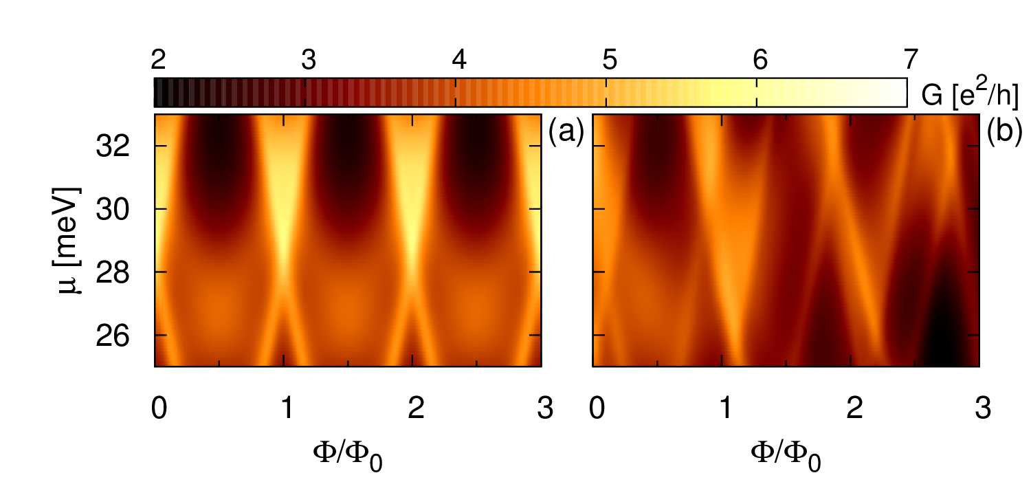
to shift the central system spectrum for a given configuration so that ground state energies match with and without impurities, in order to make possible a comparison between different impurity configurations at the same chemical potential. To demonstrate the effects of impurities on magnetoconductance, let us consider impurity configuration 1 used in Figs. 5 (a) and (c). Realigning the spectrum requires a gate voltage mV. Figure 6 shows the resulting conductance of the finite cylinder coupled to leads without (a) and with (b) spin included as a function of and . Provided the oscillations were periodic prior to the inclusion of impurities (i. e. if ) they remain so when impurities are included. This is because the impurity potentials do not couple to . The conductance curves with and without impurities [Figs. 2 (a) and (d)] are qualitatively similar, but the impurities dampen oscillation amplitudes by reducing maxima and increasing minima.

So far, we have considered the conductance of particular impurity configurations and seen that FP oscillations can survive in the presence of impurity-induced dampening. We can also evaluate the average magnetoconductance at a fixed over multiple random impurity configurations, which gives insight into the general behavior of an assembly of core-shell nanowires. We calculate over random configurations of impurities each, where is constant for a given assembly. The assumption of a constant number of impurities per configuration is justified using reported average donor densities in the core. For reference, a core donor density of cm-3, which is large assuming a GaAs core, corresponds to or impurities in the central system under consideration.[9, 10]
Figure 7 (a) compares at meV without impurities and averaged over configurations of impurities. We neglect spin for simplicity. Further averaging does not affect the results significantly. The applied gate voltage is obtained by averaging the shift of the ground state over multiple -impurity configurations. The oscillations are indeed damped, but present. Increasing the number of impurities to [Fig. 7 (b)] the amplitude drops, but the oscillations still survive. Actually, for impurities, even averaging over configurations already yields qualitatively the same as observed in Fig. 7 (b) after extensive averaging, which implies that at such high core donor concentrations the exact impurity configuration is not paramount. The damping suggests that conductance oscillations may be reduced in amplitude beyond achievable experimental resolution in extremely disordered samples. However, our simulations indicate that even in the presence of a large but realistic core-donor density, the oscillations are clearly resolvable. Finally, we mention that our model donor impurities [Eq. (29)] do not account for screening. Screening of donor impurities in the core would reduce their effects on conduction electrons and hence on both closed and open system properties. Similarly, electron-electron interaction would oppose impurity-induced localizations in the system, e. g. as in Figs. 5 (b) and (d), and hence weaken impurity effects.[15] By ignoring screening effects in the core and electron-electron interaction, our simulations thus describe “a worst-case scenario” of the electron-impurity interactions.
V Comparison with recent experimental data
In this section we compare simulations using realistic parameters with recently reported measurements performed on GaAs/InAs core-shell nanowires. Results in Ref. 9 show FP conductance oscillations superimposed on slowly-varying background oscillations in hexagonal GaAs/InAs core-shell nanowires. The background oscillations are attributed to universal conductance fluctuations. Our cylindrical model represents an idealized core-shell nanowire and neglects some aspects present in experiment, notably the hexagonal structure, shell thickness and electron-electron interaction. Out of the effects considered in this paper, we have shown that only Zeeman splitting can break the periodicity of oscillations in cylinders, e. g. Fig. 2.

Consider a cylinder with nm and nm. Figure 8 (a) shows the energy spectrum with and . Each axial mode has an energy minimum, the spin-degeneracy of which is lifted by the Zeeman term for , producing sloped “traces” of the corresponding parabolic bottoms marked with filled circles, yielding a flux-modulated DOS at a fixed energy. The energies and meV (dashed) are located between two such traces approaching the former and distancing from the latter, resulting in a monotonically increasing and decreasing DOS, respectively. This is reflected in , which Fig. 9 (a) shows evaluated at the corresponding values and meV, decreasing and increasing gradually on average, comparable to the experimental results of Ref. 9. It follows that the measured background oscillations could be explained as an interplay between the finite system length and spin. To further illustrate this effect, Fig. 8 (b) shows the cylinder spectrum with double Zeeman interaction, , and still. The slopes of the parabola-minima traces increase revealing crossings and the DOS modulation is amplified. The DOS is maximum when two such bottom-band traces cross, i. e. for just below meV, and minimum at the largest energy separation between them. Figure 9 (b) shows the corresponding conductance for and meV and reveals that the crossings manifest as peaks in background conductance oscillations.
We can apply the correspondence between crossings of traces and peaks in background oscillations to calculate the electron g-factor. A trace is formed as a function of by the energy minima of a given axial mode, described by the spectrum Eq. (7) with which yields an equation for lines, namely the traces. An intersection between two traces occurs at a particular value of when the two corresponding lines intersect. Solving for yields
| (35) |
as because only traces of opposite spin may intersect. Here, is the magnetic flux at which the lines intersect. It may be estimated from Fig. 9 as the flux at which the background conductance oscillations peak. Applying this to at meV in Fig. 9 (b), we find . If the chemical potential is known, the axial modes follow from the condition , which must hold at . For the present example, we find and which yields compared to the input value . If the chemical potential is not known, a guess of the relevant axial modes is needed.
In Figs. 9 (a) and (b) we also note a beating pattern in the conductance, which in our model arises due to Zeeman splitting causing a misalignment of the flux-parabolas at a fixed energy [Eq. (7)]. Doubling the g-factor results in a smaller beating period as a comparison between the curves at meV clearly illustrates. Beating patterns are observable in experiment, but we note that they may also be caused by other mechanisms than spin splitting. For example, electrons might occupy higher radial modes in a shell of finite thickness and hence have different effective radii, such that more than one magnetic flux is distinguishable. The superposition of the corresponding oscillations, which are periodic in their respective fluxes, would produce a beating pattern. However, previous calculations indicate that the oscillations should remain periodic in the presence of a small, nonzero shell thickness.[15, 16]
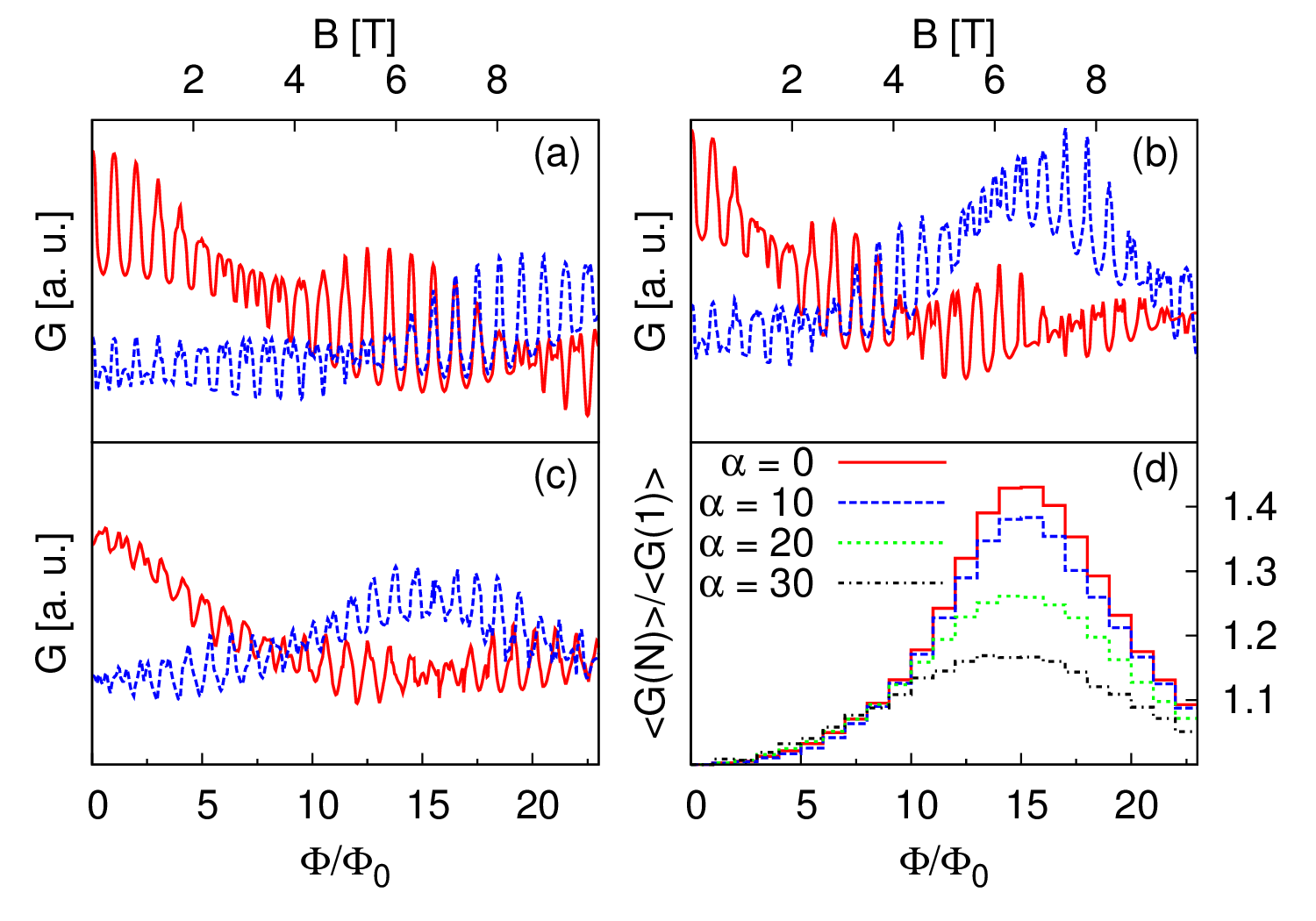
Finally, Fig. 8 (c) shows the spectrum with and meVnm. Interestingly, due to the SOI the crossings of the traces become avoided, their energy separation increasing with . The resulting energy “gap” dampens the background-oscillation peaks of , as is shown for meV at in Fig. 9 (c). Rashba SOI also dampens the FP oscillations themselves as discussed in Sec. III.4. To understand how the amplitude of the background conductance oscillations varies with , Fig. 9 (d) shows how the conductance averaged over the -th flux with varies with relative to for different values of . By averaging over the intervals between integer fluxes we exclude the -periodic part of and isolate the Zeeman-induced background oscillations. In analogy with Figs. 9 (b) and (c), peaks around and as increases the peak is reduced in amplitude relative to . It has been shown[50, 51, 52] that is controllable by applying a gate voltage and therefore measurements on peaks in the background oscillations of magnetoconductance in GaAs/InAs core-shell nanowires may allude to the existence of Rashba SOI in such tubular systems. Importantly, for the background conductance oscillations flatten, but the peaks do not shift much compared to , and so Eq. (35) may still be applied to estimate .
VI Conclusions
We performed transport calculations of electrons situated on a cylindrical surface in the presence of a longitudinal magnetic flux and obtained flux-periodic oscillations at different chemical potentials. Varying shifts the chemical potential of the system relative to the fixed spectra of the central part and the leads, similar to the experimental setup in Ref. 9, where both the nanowire and the contacts are placed on a substrate used as a back gate. An alternative model is to shift only the central system spectrum relative to the leads and some fixed chemical potential, but our calculations (not shown here) reveal that these two methods are essentially identical, with only a minor difference in level-broadening. The oscillations survive and remain periodic in the presence of impurities and occur even if the contacts do not have a uniform angular coverage of the cylindrical surface. Hence, they are robust to deviations from the ideal circular and parity symmetries in the nanowire. Furthermore, the oscillations remain flux-periodic when Rashba SOI is included. The oscillations are also still present when Zeeman interaction is included, although they cease to be flux-periodic. Instead, a rich structure of beating patterns and background oscillations is identified, the latter of which also relates to the finite system length. By analyzing these oscillations, it is possible to estimate the g-factor of the electrons in the shell and detect the presence of Rashba SOI, provided the SOI strength can be varied. Our results are in qualitative agreement with recent measurements on GaAs/InAs core-shell nanowires.
Acknowledgements.
We would like to thank Thomas Schäpers, Fabian Haas, Sigurdur Ingi Erlingsson, Llorens Serra and Thorsten Arnold for enlightening discussions. This work was supported by the Research Fund of the University of Iceland and the Icelandic Research and Instruments Funds.Appendix A Infinite cylinder eigenstates with Rashba SOI
Consider an infinitely long cylinder with Rashba SOI pierced by a longitudinal magnetic flux but no Zeeman coupling, i. e. with Hamiltonian . Since we look for spinor solutions of the form [18, 19]
| (36) |
where and . The time-independent Schrödinger equation yields
| (37) |
where we define , and . The energies are
| (38) |
where and are independent of such that . To normalize, the spinor coefficients and can be chosen as
| (39) |
and
| (40) |
which clearly satisfy , , and .
References
- [1] E. P. A. M. Bakkers and M. A. Verheijen, Journal of the American Chemical Society 125, 3440 (2003).
- [2] Y. Li, F. Qian, J. Xiang, and C. M. Lieber, Materials Today 9, 18 (2006).
- [3] C. Thelander, P. Agarwal, S. Brongersma, J. Eymery, L. Feiner, A. Forchel, M. Scheffler, W. Riess, B. Ohlsson, U. Gösele, and L. Samuelson, Materials Today 9, 28 (2006).
- [4] P. Yang, R. Yan, and M. Fardy, Nano Letters 10, 1529 (2010).
- [5] J. W. W. van Tilburg, R. E. Algra, W. G. G. Immink, M. Verheijen, E. P. A. M. Bakkers, and L. P. Kouwenhoven, Semiconductor Science and Technology 25, 024011 (2010).
- [6] R. Popovitz-Biro, A. Kretinin, P. Von Huth, and H. Shtrikman, Crystal Growth & Design 11, 3858 (2011).
- [7] T. Rieger, M. Luysberg, T. Schäpers, D. Grützmacher, and M. I. Lepsa, Nano Letters 12, 5559 (2012).
- [8] M. Jung, J. S. Lee, W. Song, Y. H. Kim, S. D. Lee, N. Kim, J. Park, M.-S. Choi, S. Katsumoto, H. Lee, and J. Kim, Nano Letters 8, 3189 (2008).
- [9] O. Gül, N. Demarina, C. Blömers, T. Rieger, H. Lüth, M. I. Lepsa, D. Grützmacher, and T. Schäpers, Phys. Rev. B 89, 045417 (2014).
- [10] C. Blömers, T. Rieger, P. Zellekens, F. Haas, M. I. Lepsa, H. Hardtdegen, O. Gül, N. Demarina, D. Grützmacher, H. Lüth, and T. Schäpers, Nanotechnology 24, 035203 (2013).
- [11] Y. Aharonov and D. Bohm, Phys. Rev. 115, 485 (1959).
- [12] N. Byers and C. N. Yang, Phys. Rev. Lett. 7, 46 (1961).
- [13] R. A. Webb, S. Washburn, C. P. Umbach, and R. B. Laibowitz, Phys. Rev. Lett. 54, 2696 (1985).
- [14] L. P. Lévy, G. Dolan, J. Dunsmuir, and H. Bouchiat, Phys. Rev. Lett. 64, 2074 (1990).
- [15] V. N. Gladilin, J. Tempere, J. T. Devreese, and P. M. Koenraad, Phys. Rev. B 87, 165424 (2013).
- [16] Y. Tserkovnyak and B. I. Halperin, Phys. Rev. B 74, 245327 (2006).
- [17] R. Winkler, Spin orbit coupling effects in two-dimensional electron and hole systems (Springer-Verlag, 2003).
- [18] A. Bringer and T. Schäpers, Phys. Rev. B 83, 115305 (2011).
- [19] B. Mehdiyev, A. Babayev, S. Cakmak, and E. Artunc, Superlattices and Microstructures 46, 593 (2009).
- [20] J. S. Sheng and K. Chang, Phys. Rev. B 74, 235315 (2006).
- [21] S. Datta, Electronic Transport in Mesoscopic Systems (Cambridge University Press, 1995).
- [22] V. Gudmundsson, C. Gainar, C.-S. Tang, V. Moldoveanu, and A. Manolescu, New Journal of Physics 11, 113007 (2009).
- [23] K. S. Thygesen, M. V. Bollinger, and K. W. Jacobsen, Phys. Rev. B 67, 115404 (2003).
- [24] S. Kurth, G. Stefanucci, C.-O. Almbladh, A. Rubio, and E. K. U. Gross, Phys. Rev. B 72, 035308 (2005).
- [25] M. Brandbyge, J.-L. Mozos, P. Ordejón, J. Taylor, and K. Stokbro, Phys. Rev. B 65, 165401 (2002).
- [26] T. Tada, M. Kondo, and K. Yoshizawa, The Journal of Chemical Physics 121, 8050 (2004).
- [27] M. Paulsson and M. Brandbyge, Phys. Rev. B 76, 115117 (2007).
- [28] M. Paulsson, (2008), arXiv:cond-mat/0210519v2 [cond-mat.mes-hall].
- [29] L. Serra and M.-S. Choi, Eur. Phys. J. B 71, 97 (2009).
- [30] A. Manolescu, T. Rosdahl, S. Erlingsson, L. Serra, and V. Gudmundsson, The European Physical Journal B 86, 1 (2013).
- [31] T. Richter, C. Blömers, H. Lüth, R. Calarco, M. Indlekofer, M. Marso, and T. Schäpers, Nano Letters 8, 2834 (2008).
- [32] A. Lorke, R. J. Luyken, A. O. Govorov, J. P. Kotthaus, J. M. Garcia, and P. M. Petroff, Phys. Rev. Lett. 84, 2223 (2000).
- [33] D. Takai and K. Ohta, Phys. Rev. B 48, 1537 (1993).
- [34] D. Takai and K. Ohta, Phys. Rev. B 49, 1844 (1994).
- [35] S. Washburn, H. Schmid, D. Kern, and R. A. Webb, Phys. Rev. Lett. 59, 1791 (1987).
- [36] M. P. Nowak and B. Szafran, Phys. Rev. B 80, 195319 (2009).
- [37] A. M. Alexeev and M. E. Portnoi, Phys. Rev. B 85, 245419 (2012).
- [38] A. van Oudenaarden, M. H. Devoret, Y. V. Nazarov, and J. E. Mooij, Nature 391, 768 (1998).
- [39] C. Daday, A. Manolescu, D. C. Marinescu, and V. Gudmundsson, Phys. Rev. B 84, 115311 (2011).
- [40] Y. Gefen, Y. Imry, and M. Y. Azbel, Phys. Rev. Lett. 52, 129 (1984).
- [41] M. Büttiker, Y. Imry, and M. Y. Azbel, Phys. Rev. A 30, 1982 (1984).
- [42] G. W. Holloway, D. Shiri, C. M. Haapamaki, K. Willick, G. Watson, R. R. LaPierre, and J. Baugh, (2013), arXiv:1305.5552v1 [cond-mat.mes-hall].
- [43] G. Ferrari, G. Goldoni, A. Bertoni, G. Cuoghi, and E. Molinari, Nano Letters 9, 1631 (2009).
- [44] D. Frustaglia and K. Richter, Phys. Rev. B 69, 235310 (2004).
- [45] F. Nagasawa, J. Takagi, Y. Kunihashi, M. Kohda, and J. Nitta, Phys. Rev. Lett. 108, 086801 (2012).
- [46] J. J. Sakurai and J. Napolitano, Modern Quantum Mechanics (Pearson, 2011).
- [47] H. S. Cohl and J. E. Tohline, The Astrophysical Journal 527, 86 (1999).
- [48] J. Segura and A. Gil, Computer Physics Communications 124, 104 (2000).
- [49] Z. Barticevic, G. Fuster, and M. Pacheco, Phys. Rev. B 65, 193307 (2002).
- [50] G. Engels, J. Lange, T. Schäpers, and H. Lüth, Phys. Rev. B 55, R1958 (1997).
- [51] J. Nitta, T. Akazaki, H. Takayanagi, and T. Enoki, Phys. Rev. Lett. 78, 1335 (1997).
- [52] D. Liang and X. P. Gao, Nano Letters 12, 3263 (2012).