Models for twistable elastic polymers in Brownian dynamics, and their implementation for LAMMPS

When setting up a coarse grained model for a polymer or biopolymer it is often useful, if not necessary, to account for its ability to both bend and twist. A notable example is that of double-stranded DNA. A first coarse grained description of DNA is to view it as a semi-flexible polymer, or a worm-like chain [1], i.e. a fluctuating elastic rod with a bending rigidity, and an associated persistence length. The latter gives a measure of the length scale along the polymer backbone over which correlations in the local direction (the tangent to the backbone) decay. For DNA in a physiologically realistic salt solution this length is 50 nm, which is significantly larger than its thickness (2.5 nm for hydrated B-DNA).

While a worm-like chain provides a simple and useful description of DNA under some conditions [1, 2, 3, 4, 5], it neglects a key elastic property of this biomolecule: its resistance to twisting. Indeed, in reality DNA is a double helix which in its relaxed state has a pitch of around 10 base pairs (in B-DNA), and over-twisting or under-twisting the helix incurs an energetic penalty [6, 7]. Twisting DNA may also lead to supercoiling [9, 10, 11], i.e. the writhing of a highly twisted filament, which can be witnessed in the everyday world when twisting up an office telephone cord. Supercoiling can be due to over or under-twisting the helical DNA, and is accordingly referred to as either positive or negative.

Supercoiling is important for DNA organisation and function within cells. Within bacteria, supercoiling helps pack the genome into the tight volume of the cell [12], and Hi-C experiments suggest that this phenomenon is also gives rise to the contact maps observed for the bacterial chromosome [13]. Furthermore, it was realised many years ago that supercoiling is naturally and generically created in vivo [14, 15, 16]: as an RNA polymerase transcribes a gene, it generates an excess of twist ahead, and a deficit behind, and this leads to, respectively, positively and negatively supercoiled domains (a Brownian dynamics simulation exploring the biophysics of this phenomenon was provided in [17]). Supercoiling is also thought to play a functional role in gene regulation [18] and transcription [19] in eukaryotes. This is because, among other things, as the DNA wraps around histones to make chromatin, each wrapping adds two units of writhe into the polymer: the interplay of this writhe with the transcriptionally-driven supercoiling just discussed could help open up the chromatin fibre as it is transcribed (or replicated) [19, 9, 20, 21]. The importance of supercoiling to intracellular DNA is also apparent from the number of key enzymes whose role is to regulate it, such as DNA gyrases, which induce negative supercoiling, and topoisomerases, which are often employed to relieve it [9].

It is therefore vital for coarse grained simulations of bacterial and eukaryotic DNA, or of naked DNA loops, to be able to treat twist and twist fluctuations accurately. The simplest way to achieve this is to endow the model DNA with a twist rigidity as well as a bending rigidity [7, 22]. Just as the bending rigidity leads to a non-zero persistence length which characterises how correlations in the backbone directions decay due to bending, the twist rigidity leads to a twist persistence length, which characterises how twist correlations decay, or, equivalently, how big twist fluctuations should be at a given temperature $T$. This twist persistence length is of the same order of, and slightly larger than, the bending persistence length, and typical estimates are between 60 and 75 nm [10, 23, 24].

There are many excellent papers in the literature which discuss how to set up a model of a twistable worm-like chain to study the dynamics of DNA when supercoiling is important [25, 26, 27, 28, 29, 30, 31, 32, 33]. Most of the Brownian dynamics simulation work on coarse grained (bead-and-spring) DNA molecules with twisting and supercoiling build on the seminal contributions in Refs. [34, 35, 36]. However, most modern, widely-used molecular dynamics codes, such as lammps [37], do not currently incorporate this force field in their source code. Furthermore, in the literature there have been a variety of approaches to study twistable elastic chains, and to our knowledge there has not been a systematic analysis of the possible Hamiltonians, and the relation between them and with the available continuum theories. Thus our goal in this work is to fill this gap and provide a detailed description of possible coarse grained Hamiltonians for twistable worm-like chains, suitable for use in Brownian or Langevin dynamics simulations. We also derive formulas for the tangent-tangent and for the twist correlation functions, and describe several possible implementations of these models in lammps.

Our work is structured as follows. In the next Section, we will review the continuum theory of elastic rods. In Sec. III, we discretise the continuum energy and show that the model in Ref. [34] provides a valid discretisation, as do other equally valid options which are formulated using appropriate combinations of dihedral potentials. Section IV contains an analytical calculation of the persistence lengths in the discrete model, together with a comparison with numerical data. Section V provides a detailed description of the implementation of some of the models introduced in Sec. III in lammps, and then in Sec. VI we compare the some simulations results with the theory. Finally, in Sec. VII we draw some conclusions, and point to some possible ways in which the current work may be applied to DNA biophysics.

A non-extensible elastic rod can be described mathematically as a “stripe” (a thin slice of a plane), whose position in space is given by the vector $\mathbf{r}(s)$ where $s$ is the distance along the rod [38]. A continuous curve in three dimensional space can be described by the Frenet-Serret frame, made up of the vector tangent to the curve $\mathbf{\hat{u}}(s)=d\mathbf{r}(s)/ds$, a normal vector $\mathbf{\hat{n}}$ which points in direction of $d\mathbf{\hat{u}}/ds$, and a binormal $\mathbf{\hat{b}}=\mathbf{\hat{u}}\times\mathbf{\hat{n}}$; the relationship between these vectors and their derivatives (i.e. a description of the rotation of the frame as one moves along the curve) is given by the Frenet-Serret equation (see Ref. [38]). Whilst a curve is uniquely defined by the tangent (the other two vectors are constructed from this), a stripe with a finite thickness requires two vectors to define it: the tangent $\mathbf{\hat{u}}(s)$ and the local normal to the plane $\mathbf{\hat{f}}(s)$ (also known as the material normal). The configuration of a stripe is described by the Darboux frame, consisting of $\mathbf{\hat{u}}(s)$, $\mathbf{\hat{f}}(s)$ and a vector $\mathbf{\hat{v}}(s)$ perpendicular to these (defined such that $\mathbf{\hat{f}}\times\mathbf{\hat{v}}=\mathbf{\hat{u}}$, so that $\mathbf{\hat{f}}$, $\mathbf{\hat{v}}$ and $\mathbf{\hat{u}}$ correspond respectively to the usual $x$, $y$ and $z$ axes); a schematic representation is given in Fig. 1. The Frenet-Serret and Darboux frames are related by

where

with $\theta$ the rotation angle between the two frames.

The path of the rod is represented by the generalized curvatures $\omega_{i}(s)$ which determine the unit vectors by the generalized Frenet-Serret [38] equation

where it can be seen that $\omega_{3}(s)ds$ is the infinitesimal angle of rotation about the direction $\mathbf{\hat{u}}(s)$, $\omega_{1}(s)ds$ is the infinitesimal rotation about $\mathbf{\hat{f}}(s)$ etc. The in-extensibility of the rod can be expressed by the condition $|d\mathbf{r}/ds|=1$. The energy for an elastic rod is given by

where $\kappa_{b1}$ and $\kappa_{b2}$ are bending rigidities and $\kappa_{t}$ is the twist rigidity (each having units of energy$\cdot$length). If the elastic rod has a circular cross section, then $\kappa_{b1}=\kappa_{b2}=\kappa_{b}$, giving

By inspection of Eq. (1) we can identify the curvature of the rod

and also

One can therefore also write the energy

The flexibility of the rod can be described by looking at correlations in the direction of the vectors along the rod. For example, the bending correlations are given by $\langle\mathbf{\hat{u}}(0)\cdot\mathbf{\hat{u}}(s)\rangle$, whereas the twist correlations are given by $\langle\mathbf{\hat{f}}(0)\cdot\mathbf{\hat{f}}(s)\rangle$. We include a simple calculation of these expressions, in the continuous limit, in Appendix A.

We now consider a discrete elastic rod model, with segments of length $a$ which are defined by the position vectors of the vertices between each segment $\mathbf{r}_{i}$, $i=1,\dots N$. The configuration of the rod can be described by the tangents $\mathbf{\hat{u}}_{i}=(\mathbf{r}_{i+1}-\mathbf{r}_{i})/a$ [39], and the orthogonal vectors $\mathbf{\hat{f}}_{i}$ and $\mathbf{\hat{v}}_{i}$. Together $\mathbf{\hat{u}}_{i},\mathbf{\hat{f}}_{i}$ and $\mathbf{\hat{v}}_{i}$ make up a frame of reference on vertex $i$.

To discretise the energy, we start from the functional in Eq. (3). By using the following discretised approximations

we obtain

To get the final formula, we have used the following mixed product identity,

which holds for any triplet of vectors, $\mathbf{a}$, $\mathbf{b}$ and $\mathbf{c}$.

Another useful parametrisation of the energy is to use Euler angles, where a set of three angles $\alpha$, $\beta$, and $\gamma$ is used to describe a rotation from one frame of reference to another. Here we use the $z\mbox{-}x^{\prime}\mbox{-}z^{\prime\prime}$ Euler angle convention where the first angle is a rotation of the initial frame about the $z$-axis, the second a rotation about the new $x$-axis, and the third about the new $z$-axis. Rotations have positive sign if they are clockwise when looking along the axis. The rotation can be written as a matrix $\mathcal{R}$, for example to rotate the reference frame on vertex $i$ to that on $i+1$, $\left(\mathbf{\hat{u}}_{i+1},\mathbf{\hat{f}}_{i+1},\mathbf{\hat{v}}_{i+1}\right)^{\rm T}=\mathcal{R}\left(\mathbf{\hat{u}}_{i},\mathbf{\hat{f}}_{i},\mathbf{\hat{v}}_{i}\right)^{\rm T}$ The matrix can be decomposed into individual rotations

where

and

are rotation matrices such that e.g. $R_{\mathbf{\hat{f}}}(\theta)\left(\mathbf{\hat{u}},\mathbf{\hat{f}},\mathbf{\hat{v}}\right)^{\rm T}$ gives a set of axis vectors which have been rotated by an angle $\theta$ about $\mathbf{\hat{f}}$.

By using angles, $\alpha_{i}$, $\beta_{i}$ and $\gamma_{i}$ to describe the rotation between vertex $i$ and $i+1$, Eq. (4) can be rewritten as

Expanding this to second order in $\beta_{i}$ and $\alpha_{i}+\gamma_{i}$ [which are both small due to the Boltzmann weight associated to the energy function in Eq. (7)], we obtain

which is the energy function proposed in Ref. [34] and used in most subsequent works. This Hamiltonian is therefore equivalent to Eq. (3) in the continuum limit, where $a\to 0$ while $\kappa_{b,t}/a$ are kept constant. In the same limit, another viable version, which we will use in the rest of this work, is

where the $\beta_{i}$ and $\alpha_{i}+\gamma_{i}$ angles are treated symmetrically.

We note that the energy for each segment is independent, and Eq. (9) can be written as a sum $E_{\rm DER}=\sum_{i}E_{i}$. A typical simulation of such a discrete rod would represent each vertex as a bead, employing a spring potential between each (e.g. a harmonic or FENE springs) to account for extension of the polymer, and a steric interaction potential to prevent beads overlapping. The total energy for the system would therefore be a sum of these components $\mathcal{H}=E_{\rm DER}+E_{\rm spring}+E_{\rm steric}$.

In this section we find correlation functions for bending and twisting along the discrete rod, similar to those described in Sec. II (see Appendix A) for the continuous case. We will therefore need to calculate the probability of a given chain configuration

where $E_{i}$ is the $i$th term of the sums in Eq. (9) and

with $\mathcal{D}(\alpha,\beta,\gamma)$ the volume element for integrating over orientations parametrised by the Euler angles. To find the correlation functions it will useful to write down a rotation or “transfer” matrix, which describes the rotation of the frame at vertex $i$ required to get that at $i+1$ [40]. Using the Euler angle formulation this is simply the matrix given in Eq. (6), i.e.

where

Alternatively we can write this as a set of equations for the $i+1$th set of vectors as functions of the $i$th

Correlation functions can be found from the Eigenvectors of the average of the transfer matrix $\langle\mathcal{R}\rangle$. The matrix elements are found, e.g. by integrating $\langle\cos\beta_{i}\rangle=\int\cos\beta_{i}\mathcal{P}(\{\mathbf{r}_{i}\})\mathcal{D}(\alpha_{i},\beta_{i},\gamma_{i})$. Since each segment decouples, i.e. $P(\{\mathbf{r}_{i}\})=\prod_{i}P_{i}(\mathbf{r}_{i})$, we can consider averages on only an individual segment, and here-on drop the $i$ index where appropriate. To perform the integrals we note that $\beta$ is in the interval $[0,\pi]$, whereas $\alpha,\gamma\in[-\pi,\pi]$; the appropriate volume element is

where $C$ is an arbitrary constant; since this will cancel out in the averages we set $C=1$. In the probability the $\beta$ terms and the $\alpha+\gamma$ terms factorize, so that $\langle\sin\beta\cos\gamma\rangle=\langle\sin\beta\rangle\langle\cos\gamma\rangle$ and $\langle\cos\beta\sin\alpha\sin\gamma\rangle=\langle\cos\beta\rangle\langle\sin\alpha\sin\gamma\rangle$ etc. Also we find that $\langle\sin\alpha\rangle=\langle\sin\gamma\rangle=\langle\cos\alpha\rangle=\langle\cos\gamma\rangle$=0, and $\langle\sin\alpha\cos\gamma\rangle=\langle\cos\alpha\sin\gamma\rangle=0$. This leaves a diagonal matrix

The partition function for a segment is

where $I_{\nu}(x)$ are the modified Bessel functions of the first kind. Evaluating the remaining matrix elements we find

To get analytic expressions for these averages we expand about $ak_{B}T/\kappa_{b}\to 0$ and $ak_{B}T/\kappa_{t}\to 0$. To first order this gives

The vectors $\mathbf{\hat{u}}_{i}$, $\mathbf{\hat{f}}_{i}$ and $\mathbf{\hat{v}}_{i}$ are eigenvectors of $\langle\mathcal{R}\rangle$. The eigenvalue corresponding to $\mathbf{\hat{u}}_{i}$ is $\langle\cos\beta\rangle$, meaning that

i.e. an exponential decay with a correlation length $\xi_{u}=-a/\ln\langle\cos\beta\rangle$. Using Eq. (18) gives

We identify this as the bending persistence length (which is the same as in the continuous case – see Appendix A).

The eigenvalue corresponding to the eigenvector $\mathbf{\hat{f}}_{i}$ is $\langle\cos\alpha\cos\gamma\rangle(1+\langle\cos\beta\rangle)$. In a similar fashion to above, we can say that

where $\xi_{f}=-a/\ln[\langle\cos\alpha\cos\gamma\rangle(1+\langle\cos\beta\rangle)]$ is the $\mathbf{\hat{f}}_{i}$ correlation length. Using Eqs. (18) and (19) and taking the small $a$ limit gives

Note that in the limit of large $\kappa_{b}$, i.e. a straight rod, the twist correlation length reduces to $\xi_{f}=2\kappa_{t}/k_{B}T$; in other cases though, this correlation length is not such a useful quantity as it measures both bending and twisting.

Other useful properties of the chain are the mean of the cosine and sine of the twist angle between a pair of segments $\langle\cos(\alpha+\gamma)\rangle$ and $\langle\sin(\alpha+\gamma)\rangle$, and also the correlation in the total twist between two points along the chain. The first two quantities are found to be

and

The latter is the mean of the cosine of the total twist between two points, $\langle\cos\Omega_{n}\rangle$, where $\Omega_{n}=\sum_{i=1}^{n}(\alpha_{i}+\gamma_{i})$ is the sum of twist angles between each of the beads from $1$ to $n$. Since $\langle\cos\Omega_{n}\rangle$ will decrease as $n$ increases, we can write $\langle\cos\Omega_{n}\rangle=e^{-na/\xi_{\rm Tw}}$, where $\xi_{\rm Tw}$ the twist correlation length. The average is given by

where $d\Gamma=\prod_{i=1}^{N}\mathcal{D}(\alpha_{i},\beta_{i},\gamma_{i})$, and $\Phi_{i}=\alpha_{i}+\gamma_{i}$. Since the integral will be the same for each $i\leq n$, and terms for $i>n$ cancel, this simplifies to

and

Using Eqs. (23) and (24) above gives

and we find $\xi_{\rm Tw}=-a/\log(1-ak_{B}T/2\kappa_{t})$. Finally, for small $ak_{B}T/\kappa_{t}$

The model described above cannot be easily incorporated into pre-existing scalable software such as the lammps molecular dynamics solver. In Ref. [34] Chirico and Langowski describe a Brownian dynamics simulation scheme for a bead-and-spring polymer model of DNA, where at each time step the positions of each bead are incremented by $\delta\mathrm{r}_{i}$ and the $\mathbf{\hat{f}}_{i}$ vectors rotated by $\delta\Phi_{i}$ about the tangents $\mathbf{r}_{i+1}-\mathbf{r}_{i}$, according to the energy given in Eq. (8) (plus terms for stretching and excluded volume). At each step they also make a correction to ensure that the $\mathbf{\hat{f}}_{i}$ vectors remain perpendicular to the tangents (i.e. $\mathbf{\hat{u}}_{i}$ are aligned along the backbone); this correction prevents a straightforward implementation of this model in lammps and other multi-purpose molecular dynamics software. Here we describe two alternative models in which we add an additional term to the energy in place of this correction.

In order to describe a bead-and-spring polymer with torsional rigidity the beads must have an orientation as well as a position. In lammps this can be achieved in two ways: either by representing each bead by a rigid body (a collection of point “atoms” which move and rotate as a unit), or by a spherical atom which has position and orientation.

We now compare the theoretical results for the correlation functions derived in Sec. IV with those from numerical simulations of bead-and-spring polymers. We use the lammps software to implement each of the models described in the previous section.

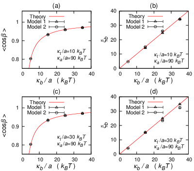
Simulations were of a bead-and-spring polymer of length $N=200$ beads. The force fields used correspond either to the Hamiltonian given in Eq. (27) or to that in Eq. (38), plus FENE spring interactions between the beads, and shifted, truncated Lennard-Jones interactions, which were used to stop the beads from overlapping. Dynamics were evolved according to the Langevin equation (a scheme commonly know as Langevin dynamics, or Brownian dynamics with no hydrodynamic interactions). Averages and correlation lengths are measured from equilibrium configurations.

In Fig. 3 the average bending angle and the bending persistence length are shown; for both models there is good agreement with theory. In Fig. 4 we show results for the twisting of the chain. This time there is a good agreement between theory and both models for averages over the individual twist angles ($\alpha+\gamma$). The long range correlation results agree less well, with the measured twist correlation length $\xi_{\rm Tw}$ slightly shorter than suggested by the theory. A likely source of this discrepancy is the fact that the Hamiltonian from which we obtain the expression for $\xi_{\rm Tw}$ does not contain the term in $\bar{\kappa}_{a}$ from the alignment interaction which is present in the simulations.

To summarise, we have discussed here a number of possible models for a twistable worm-like chain, which are suitable for use in coarse grained Brownian dynamics simulations. We have provided a detailed analysis of the connection between discretised and continuous energy functions, which shows that both standard formulations in terms of Euler angles (such as the one originally introduced in Ref. [34]), and another description based on dihedrals, are equivalent with the continuous theory up to second order in the bending and twist angles. This link is not commonly discussed in the literature, yet it is crucial to prove that the theory has the right continuous limit. In our experience it is quite easy to build up an energy function for twistable elastic rods which has the right behaviour for straight fibres, but does not obey the correct continuum theory when bending and twist fluctuations are simultaneously incorporated. Our explicit analysis provides a simple criterion to discriminate between viable and non-viable theories. Furthermore, we have shown that, as expected, all “correct” models possess well-behaved tangent-tangent and twist correlation functions, associated with two different persistence lengths.

The continuum description of an elastic rod in Sec. II has been formulated for a linear rod with unconstrained ends. Several previous studies [22, 46] have focused on supercoiled DNA by considering a rod stretched between two substrates; there the rod is parametrised by the deviation of its configuration from a reference relaxed molecule, an extra stretching term is included in the energy, and a constraint of constant linking number is imposed. That description suffers from a pathology in the continuum limit which arises because twisting a constrained rod will lead to writhing, and, unless self-avoidance is accounted for, it is possible for loops to form and the rod to pass through itself (this manifests as a singularity in the constant linking number Hamiltonian, and is related to the analogous system of a quantum mechanical symmetric top [22]). This problem does not arise in our analytical treatment, because we do not need to employ any approximate formulas for writhe and linking number, as we do not include supercoiling (since the ends of the rod are not constrained). A similar pathology appears in the case where the energy includes a term in the geometric normal $\mathbf{\hat{n}}$ (defined in Sec. II) instead of the material normal $\mathbf{\hat{f}}$ [40], which gives rise to complex eigenvalues of the transfer matrix; this results in the tangent-tangent correlations decaying in an oscillatory way, with the oscillation period becoming singular in the continuum limit. We do not encounter this problem in the present work, since the energy in Eq. (9) leads to a transfer matrix [Eq. (16)] with real eigenvalues.

The main contribution of our work is that we have provided a detailed implementation of the model of Refs. [34] in LAMMPS [37], a very well used code to simulate Brownian dynamics. The associated code, which is available on request, allows the inclusion of Hamiltonians defined in terms of Euler angles, and we expect it will be of use in the future to perform large scale and parallel coarse grained simulations of DNA and of other polymers or fibres where twist, as well as twist fluctuations, play a major role in the physics (for some examples, see e.g. Refs. [47, 48]).

In particular, one may use the implementation we have described to study the dynamics and physics of confined supercoiled DNA, which is a good starting point to describe bacterial DNA; it would also be possible, for instance, to model supercoiling in chromatin fibres and chromosome fragments, to begin understanding its role in gene regulation. The advantage of the approach we are proposing here is that, thanks to the high scalability of LAMMPS, these simulations can reach unprecedented large scale with respect to previous simulations of coarse grained supercoiled DNA presented.

References

- [1] J. F. Marko and E. D. Siggia, Macromolecules 28, 8759 (1995).
- [2] C. Bustamante, J. F. Marko, E. D. Siggia and S. Smith, Science 265, 1599 (1994).
- [3] P. L. Hansen and R. Podgornik, J. Chem. Phys. 114, 8637 (2001).
- [4] A. Rosa, T. X. Hoang, D. Marenduzzo and A. Maritan, Macromolecules 36, 10095 (2003).
- [5] N. M. Toan, D. Marenduzzo, C. Micheletti, Biophys. J. 89, 80 (2005).
- [6] C. R. Calladine and H. Drew, Understanding DNA, Academic Press, San Diego (1992).
- [7] J. F. Marko and E. D. Siggia, Science 265, 506 (1994).
- [8] J. F. Marko and E. D. Siggia, Macromolecules 27, 981 (1994).
- [9] N. Gilbert and J. Allan, Curr. Opin. Gen. Devel. 25, 15 (2014).
- [10] J. F. Marko and E. D. Siggia, Phys. Rev. E 52, 2912 (1995).
- [11] S. Forth, C. Deufel, M.Y. Sheinin, B. Daniels, J.P. Sethna, and M.D. Wang, Phys. Rev. Lett. 100 148301 (2008).
- [12] L. Postow, C. D. Hardy, J. Arsuaga and N. R. Cozzarelli, Gen. Devel. 18, 1766 (2004).
- [13] T. B. K. Le, M. V. Imakaev, L. A. Mirny and M. T. Laub, Science 342, 731 (2013).
- [14] L. F. Liu and J. C. Wang, Proc. Natl. Acad. Sci. USA 84, 7024 (1987).
- [15] Y. P. Tsao, H. Y. Wu and L. F. Liu, Cell. 56, 111 (1989).
- [16] S. Deng, R.A. Stein, and N.P. Higgins, Molecular Microbiology 57 1511 (2005).
- [17] S. P. Mielke, W. H. Fink, V. V. Krishnan, N. Groenbech-Jensen and C. J. Benham, J. Chem. Phys. 121, 8104 (2004).
- [18] C. Naughton et al., Nat. Struct. Mol. Biol. 20, 387 (2013).
- [19] D. J. Clark and G. Felsenfeld, EMBO J. 10, 387 (1991).
- [20] J. Roca, Chromosoma 120 323 (2011).
- [21] N. Mondal and J.D. Parvin, Nature 413 435 (2001).
- [22] C. Bouchiat and M. Mézard, Eur. Phys. J. E 2 377 (2000).
- [23] B. S. Fujimoto and J. M. Schurr, Nature 344 175 (1990).
- [24] J. Lipfert, J.W.J. Kerssemakers, T. Jager, and N.H. Dekker, Nat Meth 7 977 (2010).
- [25] T. R. Powers, Rev. Mod. Phys. 82, 1607 (2010).
- [26] W. K. Olson, Curr. Opin. Struct. Biol. 6, 242 (1996).
- [27] R. K. Z. Tan and S. C. Harvey, J. Mol. Biol. 205, 573 (1989).
- [28] G. C. Rollins, A. S. Petrov, and S. C. Harvey, Biophys. J. 94, L38 (2008).
- [29] T. A. Knotts, N. Rathore, D. C. Schwartz and J. J. de Pablo, J. Chem. Phys. 126, 084901 (2007).
- [30] J. Huang, T. Schlick and A. Vologodskii, Proc. Natl. Acad. Sci. USA 98, 968 (2001).
- [31] T. Schlick and W. K. Olson, Science 257, 1110 (1992).
- [32] T. Schlick, Curr. Opin. Struc. Biol. 5, 245 (1995).
- [33] S. Rappaport and Y. Rabin, Macromolecules 37, 7847 (2004).
- [34] G. Chirico and J. Langowski Biopolymers 34, 415 (1994).
- [35] G. Chirico and J. Langowski Biophys J. 71, 955 (1996).
- [36] S. Allison, R. Austin and Mike. Hogan, J. Chem. Phys. 90, 3843 (1989).
- [37] S. J. Plimpton, J. Comp. Phys. 117, 1 (1995) (http://lammps.sandia.gov).
- [38] S. M. Rappaport and Y. Rabin J. Phys. A 40, 4455 (2007).
- [39] In the case of a linear rod there are position vectors describing the vertices of segments, with tangents with . For a circular rod there are segments and
- [40] D. Marenduzzo, C. Micheletti, H. Seyed-allaei, A. Trovato and A. Maritan, J. Phys. A 38, L277 (2005).
- [41] F. Benedetti, J. Dorier, Y. Burnier, and A. Stasiak, Nucl. Aci. Res. 42 2848 (2013).
- [42] C.A. Brackley, J. Allan, D. Keszenman-Pereyra and D. Marenduzzo, Submitted (2014).
- [43] The two potentials are however equivalent in the limit where all of , and are small, a regime which is forced by the Hamiltonian considering either of the dihedrals.
- [44] The angles are minimised by choosing a large alignment energy ; in practice this can be set as large as possible subject to numerical stability.
- [45] Source code for the lammps orientation angle style discussed in section V.2 is available on request from the authors.
- [46] J. D. Moroz and P. Nelson, Proc. Nat. Acad. Sci. 94, 14418 (1997).
- [47] S. A. Koehler, T. R. Powers, Phys. Rev. Lett. 85, 4827 (2000).
- [48] C. W. Wolgemuth, T. R. Powers and R. E. Goldstein, Phys. Rev. Lett. 84, 1623 (2000).
- [49] R. D. Kamien, Rev. Mod. Phys. 74, 953 (2002).
- [50] G. H. Fredrickson, The equilibrium theory of inhomogeneous polymers, Oxford University Press, New York (2006).
- [51] If is a rotation matrix for rotating a vector by an angle about some axis , then . In the limit , .