Polarized Curvature Radiation in Pulsar Magnetosphere
Abstract
The propagation of polarized emission in pulsar magnetosphere is investigated in this paper. The polarized waves are generated through curvature radiation from the relativistic particles streaming along curved magnetic field lines and co-rotating with the pulsar magnetosphere. Within the emission cone, the waves can be divided into two natural wave mode components, the ordinary (O) mode and the extraordinary (X) mode, with comparable intensities. Both components propagate separately in magnetosphere, and are aligned within the cone by adiabatic walking. The refraction of O-mode makes the two components separated and incoherent. The detectable emission at a given height and a given rotation phase consists of incoherent X-mode and O-mode components coming from discrete emission regions. For four particle-density models in the form of uniformity, cone, core and patches, we calculate the intensities for each mode numerically within the entire pulsar beam. If the co-rotation of relativistic particles with magnetosphere is not considered, the intensity distributions for the X-mode and O-mode components are quite similar within the pulsar beam, which causes serious depolarization. However, if the co-rotation of relativistic particles is considered, the intensity distributions of the two modes are very different, and the net polarization of out-coming emission should be significant. Our numerical results are compared with observations, and can naturally explain the orthogonal polarization modes of some pulsars. Strong linear polarizations of some parts of pulsar profile can be reproduced by curvature radiation and subsequent propagation effect.
Keywords:
curvature radiation - rotation - relativistic particles - pulsars: general1 INTRODUCTION
Polarized pulse profiles are the key observations to understand the physical processes within pulsar magnetosphere. Various polarization features have been observed (Lyne & Manchester, 1988; Rankin & Ramachandran, 2003; Han et al., 1998; Han et al., 2009, e.g.). The linear polarizations are dominating for whole or some parts of profiles, reaching such as Vela and PSR B1737-30 (Wu et al., 1993). The position angles (PA) of linear polarization often follow S-shaped curves, which has been well explained by the Rotating Vector Model (RVM) (Radhakrishnan & Cooke, 1969). Some pulsars exhibit two orthogonally polarized modes in the PA curves, where a jump is accompanied by low linear polarization (Stinebring et al., 1984; McKinnon & Stinebring, 2000). The circular polarizations of integrated profiles are usually weak (less than ) and diverse (Han et al., 1998). There exist two main types of circular polarization signature: the antisymmetric type with a sign reversal in the mid-pulse and the symmetric type without sign changes over the whole profile (Radhakrishnan & Rankin, 1990).
To understand these diverse polarization features, there have been a lot of theoretical works on pulsar emission processes and propagation effects in pulsar magnetospheres. Pulsar radio emission is generally believed to be coherent radiation from relativistic particles streaming along the open magnetic field lines in pulsar magnetosphere. The coherence can be caused either by the stable charge bunches (‘antenna’ mechanism, e.g. Benford & Buschauer (1977)) or by the instabilities (‘maser’ mechanism) including the curvature plasma instability (Beskin et al., 1988), two-stream instability (Kazbegi et al., 1991, e.g.), the beam-plasma instability induced by the curvature drift (Luo et al., 1994), etc. Various models have been constructed based on these two coherent manners (Beskin et al., 1988; Xu et al., 2000; Gangadhara, 2010, e.g.). Among these models, curvature radiation from charge bunches serves as one of the most probable mechanisms, whose coherent process, luminosity and spectrum have been investigated already (Buschauer & Benford, 1976; Benford & Buschauer, 1977; Ochelkov & Usov, 1980, e.g.). Its polarization features are the most important base for theoretical considerations. Gil & Snakowski (1990) pointed out that the curvature radiation can lead to the sign reversal feature for circular polarization of the core component. By incorporating rotation effects, Blaskiewicz et al. (1991) studied the phase lag between the centers of the PA curve and the intensity profile. Gangadhara (2010) considered the detailed geometry for curvature radiation and explained the correlation between the PA and the sign reversal of circular polarization. Recently, Wang et al. (2012) and Kumar & Gangadhara (2012) independently considered the co-rotation effect and the emission geometry, and demonstrated that the circular polarization can be of a single sign or sign reversals depending on the density gradient of particles along the rotation phase.
In addition to the emission process, propagation effects may also have significant influences on pulsar polarizations. The plasma within pulsar magnetosphere has two orthogonally polarized transverse modes, the ordinary mode (O-mode) and the extraordinary mode (X-mode) (Melrose & Stoneham, 1977; Arons & Barnard, 1986; Beskin et al., 1993; Wang & Lai, 2007, e.g.). When emission leaves the magnetosphere, it is coupled to these two modes. As the emitted waves propagate outward, they first experience the “adiabatic walking”, i.e., with their polarization following the direction of the local magnetic field (Cheng & Ruderman, 1979). Then, with the change of plasma conditions, the “wave mode coupling” occurs near the polarization limiting radius where the mode evolution becomes non-adiabatic, which will results in circular polarization (Cheng & Ruderman, 1979; Petrova, 2006; Wang et al., 2010). As the waves propagate further to the far magnetosphere, the “cyclotron absorption” takes place, which will lead to intensity absorption and net circular polarization if the distributions of electrons and positrons are asymmetric (Luo & Melrose, 2001; Petrova, 2006; Wang et al., 2010). Moreover, unlike the rectilinear propagation for the X-mode waves, the O-mode waves will undergo refraction additionally in the near regions of their generation (Barnard & Arons, 1986; Lyubarskii & Petrova, 1998), which makes the two components separated finally.
These physical processes within pulsar magnetosphere have been studied for the emission generation and propagation. However, the joint researches for emission and propagation to explain observational facts are rare. As the first try, Cheng & Ruderman (1979) considered the emission of the relativistic particles subjected to parallel and perpendicular (compare to local magnetic field) accelerations, and demonstrated the influence of “adiabatic walking” on the ordering of the polarization vectors within the emission cones. They found that the combination for emission in the inner magnetosphere and propagation effects in the outer magnetosphere can naturally explain the observed polarization and the sudden orthogonal mode transitions observed for the individual pulses. However, they did not consider the rotational effect of the relativistic particles and the refractions for the O-mode waves. The beamed emissions within the emission cone were improperly treated as coherent radiations. Wang et al. (2012) depicted the most detailed pictures of curvature radiation, but propagation effects are not included yet. Wang et al. (2010) and Beskin & Philippov (2012) studied the influences of the propagation effects on the mean profiles, but the intensity and polarization of the emitted waves were assumed rather than calculated from the emission mechanisms. Stimulated by these researches, we focus on the general picture for the combined effects of curvature radiation and propagation effects, and tries to tie the theoretical explanation with polarization observations.
In this paper, we study the polarization features of the emission generated by curvature radiation and their modifications during wave propagation in pulsar magnetosphere through numerical calculations and simulations. The paper is organized as follows. In Section 2, we present the theoretical grounds of curvature radiation and propagation effects for our calculations. Polarized emission within the cone and the evolution of two separated natural modes in magnetosphere are studied in Section 3. In Section 4, the intensities of both modes within the entire pulsar beam are calculated for the density models of uniformity, cone, core and patches. Discussion and conclusions are given in Section 5.
2 Theoretical basics for curvature radiation and propagation
2.1 Curvature radiation process

In general, pulsar magnetosphere has an inclined dipole magnetic field, which rotates uniformly in free space,
| (1) |
here is the magnetic field on the neutron star surface, is the neutron star radius, is the unit vector along , and represents the unit vector of the magnetic dipole moment, as shown in Fig. 1. According to Ruderman & Sutherland (1975), relativistic particles are generated in the vacuum gaps above the polar caps of pulsar magnetosphere by the sparking process and streaming out along the open magnetic field lines. Due to the bending of the field lines, the relativistic particles will experience perpendicular acceleration and produce curvature radiation. The coherent bunches of the relativistic particles are simply treated as huge point charges.
For a relativistic particle traveling with velocity along an open field line, its radiation field in direction and the corresponding Fourier components have been depicted in detail by Wang et al. (2012). The energy radiated per unit frequency per unit solid angle reads (Jackson, 1975)
| (2) | |||||
Here is the distance between the trajectory center and the observer, is the curvature radius for the particle trajectory, Lorentz factor , is the angle between the emission direction and the particle velocity , , and are the modified Bessel functions of the second kind.
2.2 Propagation effects
Immediately after the electromagnetic waves were generated through curvature radiation from the relativistic particles, they will be coupled to the local plasma modes to propagate outwards from the emission regions. For the sake of simplicity, the plasma within the magnetosphere is assumed to be cold and moves with a single velocity . The plasma is also assumed to have a density of , where is the multiplicity factor, represents the Goldreich-Julian density (Goldreich & Julian, 1969). In general, there are four wave modes within the plasma of pulsar magnetosphere (Beskin et al., 1993; Beskin & Philippov, 2012), two transverse and two longitudinal waves. Three out of them were commonly investigated (Arons & Barnard, 1986, e.g.), which are the X-mode with refraction index , the sub-luminous O-mode with and the super-luminous O-mode wave with . The subluminous O-mode (or the Alfven O-mode wave) tends to follow the field lines and suffers serious Landau damping (Barnard & Arons, 1986; Beskin et al., 1988), which will make this mode invisible. Only the X-mode and superluminous O-mode (hereafter O-mode for simplicity) can propagate outside the magnetosphere. These two modes have different evolution behaviors for the trajectories and polarizations.
2.2.1 Refraction of O-mode
The X-mode waves are always the transverse ones and propagate rectilinearly. It is convenient to analyze the propagation process in the fixed -frame, as shown in Fig. 1. Here, the -axis is set along the wave vector , e.g., the direction for the sight line . Let the parameters with subscript “i” denote the quantities at the emission point. At an instant time , one photon has traveled over a distance of along the ray from the emission point. The position vector and the pulsar rotation phase can be written as
| (3) |
here, denotes the light cylinder radius. The plasma conditions, such as the density , the magnetic field , and hence the dielectric tensor vary along the trajectory.
The O-mode wave evolves in a different manner. Refractive index of the O-mode wave is not so close to the unity as the X-mode, especially near the emission region with higher plasma density, which means that it will be deflected away from the magnetic axis. When the O-mode wave propagates outside to the low density region, the refraction effect becomes weaker and weaker, and the trajectory gets more close to the straight line just as the X-mode (Barnard & Arons, 1986; Lyubarskii & Petrova, 1998; Beskin & Philippov, 2012). The trajectory for the O-mode wave can be described by the Hamilton equations. With the dispersion relation of the mode taken into account, the Hamilton equations become (Barnard & Arons, 1986),
| (4) |
here, is the unit vector aligned with the magnetic field, represents the three dimensional refractive index, is the refractive index along the magnetic field, with the plasma frequency , , , and with .

By solving the Hamilton equations in the 3-dimensional magnetosphere, we obtained the refractive index for the O-mode wave and the refraction angle (the angle between and initial emission direction) along the ray, as shown in Fig. 2. Near the emission region, the refractive index of the O-mode wave , and the wave is deflected away from the emission direction. When the photon propagates outwards, the refraction effect can be neglected when , and then the O-mode trajectory becomes rectilinearly, i.e., with almost the fixed angle compared to the initial emission direction. The transition happens at the refraction-limiting radius (RLR), , where according to Barnard & Arons (1986). It is redefined numerically as , as indicated in Fig.2. Furthermore, high frequency emission is less refracted during its propagation, as shown in panels (a) and (b). In addition, if the plasma within pulsar magnetosphere is thin (a small ) and streams with a relatively larger velocity (a large Lorentz factor ), the O-mode wave will be less affected by the refraction process, as shown in Fig.2 (b), (c), (e) and (f). For the reasonable parameters chosen in Fig.2, the refraction-limiting radius are about 50–200 and the final refraction angles are –. In summary, our 3-D refraction calculation confirms the results from the traditional 2-D treatment, in which only the refraction within a fixed field line plane is considered (Barnard & Arons, 1986; Beskin et al., 1988; Lyubarskii & Petrova, 1998; Beskin & Philippov, 2012, e.g.).

As demonstrated above, if the low frequency O-mode wave (small ) travels through the dense (large ) and/or less relativistic (small ) plasma within pulsar magnetosphere, they will experience sufficient refraction. On the contrary, the X-mode wave travels rectilinearly regardless of the plasma conditions. Hence, for a given sight line at a fixed rotation phase, the observed emissions of X-mode and O-mode originate from two discrete regions separated by at a given emission height. As well known, pulsar radiations are coherent. To get efficient coherency, it requires the scale of particle bunches to be much smaller than the wave length of the emitting waves. Fig. 3 shows how the separation of the emission points for the two modes (in unit of the curvature-radiation wave-length or the plasma oscillation wave length ) varies with plasma density and Lorentz factor . Obviously, the separation are much larger than the wave length , especially for larger and smaller . Moreover, the bunching are induced by the plasma oscillation with a wave length . The separation is also significantly larger than . Therefore, the observed X-mode and O-mode waves at a fixed rotation phase are incoherent, which means the observed radiation should be the incoherent superposition of the two modes from two discrete emission regions.
2.2.2 Adiabatic walking
 |
 |
 | |||||
 |
 |
 |
 |
 |
 | ||
 |
 |
 |
 |
 |
 | ||
 |
 |
 |
 |
 |
 | ||
In addition to the ray trajectories, the polarization evolution of X-mode and O-mode waves should be investigated. By knowing , , and the dielectric tensor along the trajectory, we can use the wave equation
| (5) |
to describe the evolution of the polarization states. By keeping the first order terms for the transverse components of the electric field, the wave equation (Eq. 5) can be simplified and expressed as the evolution equation for the eigenmode magnitudes (Wang et al., 2010)
| (6) |
here, with the orientation of the plane , . To further investigate the evolution process, it is useful to define the adiabatic parameter (Wang et al., 2010),
| (7) |
In the inner magnetosphere, the adiabatic condition is easily to be satisfied, which means the polarization vector of the X-mode wave keeps to be orthogonal to the local plane, while that of the O-mode wave is within the plane. This is called the “adiabatic walking” process, during which mode amplitudes keep constant along the ray while the polarization state of each mode varies with magnetic field line. This kind of behavior for the “adiabatic walking” was first investigated by Cheng & Ruderman (1979) to explain the sub-pulse polarization. As the waves travel to higher magnetosphere, gradually decreases and finally becomes less than 1. The radius for is named as being the polarization limiting radius (PLR). Near this radius, the wave-mode coupling happens, one mode leaks to the other and vice verse, and hence circular polarization may be generated. In the region further that , the mode evolution becomes non-adiabatic, the polarization states of waves are frozen and would not be affected by the plasma (except for the possible cyclotron absorption). Generally the polarization limiting radius, , is quite far away from the emission point (Wang et al., 2010). We here focus on the influences of the initial propagation near the emission region, i.e., the “adiabatic walking” process.
3 Emission and propagation for the polarized waves within the cone
A relativistic particle traveling along a curved field line will beam its radiation around the velocity direction, forming a emission cone. The observed radiations at a fixed rotation phase are contributed by the particles not only at the central tangential emission point (with velocity pointing towards the observer), but also on the field lines within an angle of . In this section, we will calculate the initial intensity and polarization distributions in the emission cone and analyze the polarization evolution of the cone.
3.1 Emission cone without co-rotation
 |
 |
 | |||||
 |
 |
 |
 |
 |
 | ||
 |
 |
 |
 |
 |
 | ||
 |
 |
 |
 |
 |
 | ||
Consider the curvature radiation generated by the relativistic particles without rotation, i.e., . In this case, the acceleration vector of particles locates inside the curved magnetic field line plane. Fig. 4(a) shows the distribution of the electric field vectors in the emission cone at a given rotation phase of , , and . Due to nearly the same accelerations within the cone, are pointing towards almost the same direction at a given rotation phase. The electric fields could be decomposed into O-mode components, , and X-mode components, , as shown in the panels of Fig. 4 (b) and (c). The magnitudes for the O-mode components reach their maximum only in the central magnetic field line plane of each emission cone, where always approach zero. However, in the central plane orthogonal to the central magnetic field line plane, components reach the maximum, while the components go to almost zero.
Once the polarized waves are generated, they leave the emission region. The trajectory and polarization evolution of a single wave have been described in the previous analysis. For the emitted waves within the cone, their polarizations are greatly affected by the “adiabatic walking” during the initial propagations. The polarization evolutions of the emitted waves are shown in panels below Fig. 4(b) for X-mode components and Fig. 4(c) for O-mode components. When the waves are generated at , the polarization vectors for the X-mode components distribute symmetrically around the central tangential emission point (with ). Due to the bending of the field lines, the tangential point will gradually evolve out of the cone as the waves propagate outwards. When the waves propagate to about the distance , their polarization vectors are tending to be aligned. O-mode components experience the similar adiabatic walking as X-mode, as shown in the panels below Fig. 4(c). Finally, the O-mode electric field components are ordered to point towards the central plane (at ), which is orthogonal to that for the X-mode waves. The difference is that the trajectories of O-mode components are refracted during the initial propagations, which make the emission cones of X-mode and O-mode separated. Note that the final total intensity of the cone are almost the same for X-mode and O-mode components, which would cause strong depolarization for the final polarization profiles. We conclude therefore that without co-rotation the polarized emission generated in the inner magnetosphere can be completely depolarized.
3.2 Emission cone with co-rotation

(a) Uniform density.

(b) Conal density.

(c) Core density.
(d) Patch density.
 |
 |
 |
 |
| (a) Uniform density. | (b) Conal density. | (c) Core density. | (d) Patch density. |
The relativistic particles in pulsar magnetosphere not only stream along the magnetic field lines, but also co-rotate with the magnetosphere, i.e., with . In this case, the curvature radiation should be different because of the additional co-rotation velocity and acceleration. The emission process with was first investigated by Blaskiewicz et al. (1991) to calculate the emissions from the tangential emission points, i.e., the beam centers. Wang et al. (2012) and Kumar & Gangadhara (2012) further analyzed the analysis to the emissions within the entire cone. Fig. 5(a) demonstrates the co-rotation-considered curvature emission within the cone, showing the distribution of electric field vectors , their O-mode and X-mode components ( and ). In general, the electric fields within each cone are pointing towards almost the same direction at a given rotation phase. However, due to the rotation induced aberration, the emissions are shifted to the early rotation phases. It leads that the symmetry breaks for the patterns of about the central rotation phase . Furthermore, the polarization patterns for and also changed, as shown in the panels of Fig. 5(b) and (c). Compared with the patterns without rotation (Fig. 4), the central tangential point (where ) lies out of the cone even at the emission position due to the rotation induced aberration. After the adiabatic walking, the two components are ordered to almost the same direction and orthogonal with each other (see the panels below Fig. 5(b) and (c)). These X-mode and O-mode patterns just keep the polarization features of the left part of the corresponding emission cones without rotation. The final total intensity of the cone are quite different for the X-mode and O-mode components due to the co-rotation induced distortion to the emission cone patterns. Thus the observed mixed profiles would show strong net linear polarization, which is very different from the case without co-rotation.
4 Pulsar emission beams of two orthogonal modes
In addition to the analysis of emission and propagation for a single photon and the waves within the emission cone, we now investigate the entire pulsar emission beam to get the polarization pulsar profiles. For a given point within pulsar beam, the observed radiation is the integration of all the emissions within the cone around the tangential direction. Here we consider the emission from a fixed direction with a sight line angle and a rotation phase . Since the typical size of the emission cone is much larger than the size of the coherent particle bunch, incoherent addition of the radiations within the cone is reasonable. The total intensity for the integrated emission reads,
| (8) |
Here, (, ) is the central direction of the emission cone, while and denote the boundary for the cone, represents the density distribution for the plasma within pulsar magnetosphere. We can get pulsar beam patterns by calculating the emission intensity in every direction.
4.1 Emission beams without co-rotation

(a) Uniform density.

(b) Conal density.

(c) Core density.
(d) Patch density.
 |
 |
 |
 |
| (a) Uniform density. | (b) Conal density. | (c) Core density. | (d) Patch density. |
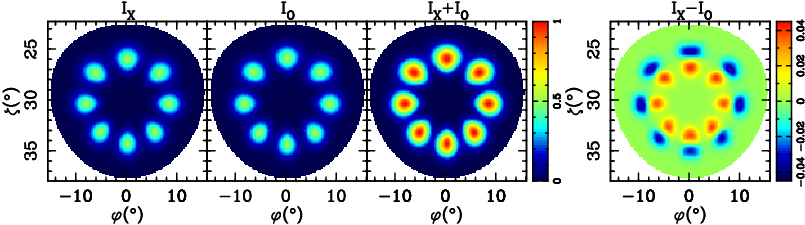
Using equation (8), we can calculate the polarization emissions from the whole open field line region without considering the co-rotation of the relativistic particles. Fig. 7 shows the calculated intensity and polarization beams for the four density models of the out-flowing particles in the form of uniformity, cone, core and patches. For the emission at a given point of pulsar beam, the X-mode and O-mode components ( and ) have a similar intensity due to the quasi symmetric geometry of the magnetic field geometry within the emission cone. Furthermore, as mentioned previously, the X-mode waves propagate rectilinearly, while the O-mode waves suffer refraction. Hence, the patterns for and are slightly different due to the refraction. Generally speaking, the O-mode image is larger than that for the X-mode. For the moderate plasma parameters used in the calculations, the refraction effect is weak and the refraction induced differences are hard to see directly from the patterns for and . However, it becomes clear from the intensity differences , which are shown in the right panels. They demonstrate the outward shift of with respect to due to refraction. If there is no refraction, will almost be zero for the entire beam.
For the uniform density model with in the open field line region at a given emission height, the emission patterns are shown in Fig. 7(a). As we see, and are stronger in the outer parts of pulsar beam where the curvature radii for the particle trajectories are smaller and curvature radiation should be stronger naturally. In addition, due to the refraction induced outward bending of the O-mode trajectories, the intensity differences, , keep to be positive for almost all parts of the beam. Their largest difference is in Fig. 7 for the typical parameters. Hence, the emergent radiation suffers serious depolarization due to the incoherent addition of the two orthogonal modes, as shown in Fig. 7(a). The net polarization within the entire beam is of X-mode.
The out-flowing particles can have a variable distribution in the polar and azimuthal directions in the magnetic axis frame, i.e., . The density models for the particles in the form of cone, core and patches have been widely used in the studies of pulsar emissions (Wang et al., 2012; Beskin & Philippov, 2012, e.g.). The conal shaped density model can be defined on the neutron star surface and extended to the high magnetosphere, described as,
| (9) |
Here, , is the polar angle of a field line footed on the neutron star surface, represents the polar angle maximum, i.e., the polar angle for the last open field line footed on the neutron star surface. For the conal density model, the intensities of the emitted wave are shown in Fig. 7(b). Obviously the emissions are peaked at the density cone for both X-mode and O-mode components. The intensity differences, , exhibit sense reversals due to the refraction of the O-mode component. Therefore, the net polarization exhibits mode jumps twice when a sight line cuts across the beam, as shown in Fig. 7(b) for , , , , and . Note that the X-mode dominates the central parts of the polarization profiles while O-mode dominates the two profile wings. Only for a sight line cutting across the edge part of the cone, for example, , the pure O-mode polarization can be detected.
The core density model can also be described by Eq. 9 except with , the emission patterns and pulse profiles for which are shown in Fig. 7(c) and Fig. 7(c). The intensity distribution of both X-mode and O-mode components are similar as those for the conal density model. The intensity near the beam center is still very weak. Because the curvature radiation intensity is still negligible due to the very large curvature radii (infinity for the central point which stands for the magnetic axis), although the density for the particles is peaked at the beam center.
The patch density model can also be described by Eq. 9, except that . Here, represents the position for the density patch in the magnetic azimuth direction and is the characteristic width of the patch. For the eight density patches located at different azimuthal directions around the magnetic axis, their emission patterns and pulse profiles are shown in Fig. 7(d) and Fig. 7(d). The X-mode components are stronger in the central regions near the magnetic axis, while the O-mode components are stronger in the outer parts of pulsar beam, as shown by the pattern for . The refraction behaves similarly as in the density cone.
To summarize, the refraction will bend the O-mode components to the outer parts of the open field line region. It leads the intensity differences for the X-mode and O-mode components at a given position and hence causes serious depolarization. Generally the X-mode dominates the central parts of the beam while the O-mode dominates the outer parts.
4.2 Emission beams with co-rotation
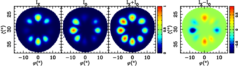
When the relativistic particles stream out in pulsar magnetosphere, the influences of co-rotation on the emissions can not be ignored. Here, we calculate the emissions of particles in the whole open field line region for the density models of uniformity, cone, core and patches. The results are shown in Fig. 8 and Fig. 9.
For the uniform density model, the total intensities, , are stronger at the edge parts of the beam, similar as the case without rotation. However, due to the rotation-induced bending of the particle trajectories, the pattern for is not symmetric around the beam center, the leading part is stronger than the trailing part. The X-mode components, , are stronger at the two sides of the beam in the direction, while the O-mode components are stronger at the two sides of the beam in the direction. Hence, the intensity differences, , show quadruple features. When sight lines of different angles of cut across the beam, various profiles are shown in Fig. 9(a). For the profiles detected by the sight lines except , the X-mode component appears at the central rotation phase, while the O-mode component emerges at two sides of the profiles.
For the conal density model, the emissions are mainly detected near the density cone (see Fig. 8b). When the sight lines cut across the central part of the beam (e.g. and ), the two intensity peaks are dominated by O-mode components with a high linear polarization (see Fig. 9b). However, when the sight lines cut across the edge parts of the beam, e.g. or , X-mode dominates the single intensity peak. For a modest , e.g. and , the polarization profile shows changes of modes as “O X O” in phases, with the X-mode dominating the central part and the O-mode the two profile wings. This “O X O” structure of the mean profile was also predicted by Beskin & Philippov (2012), and also comparable to observations (Beskin et al., 2013; Wang, 2014).
For the core density model, the emission patterns and pulse profiles are shown in Fig. 8(c) and Fig. 9(c). Unlike the emissions from the particles without rotation, the relativistic particles traveling along the central magnetic field lines also produce considerable radiation. The emission direction is bent towards the rotation direction with the dominating O-mode. When sight lines cut across the beam, the X-mode emission is detected in the central part, and the O-mode emissions from the two sides.
For eight density patches located on pulsar polar cap, the emission beam patterns and pulse profiles are shown in Fig. 8(d) and Fig. 9(d). The distributions of , , , and for the eight density patches are similar as those discrete parts of the density cone.
In summary, the rotation has significant influences on pulsar emission beam and polarization. It causes the emissions of the leading components stronger than the trailing ones. Though PA curves are quite similar to these without rotation, the pulse profiles have significant polarization in some parts, different from the case without rotation.
5 Discussions and Conclusions
In this paper, we have investigated the emission and the propagation of a single photon, the waves within the emission cone, and the emission within the entire open field line region. The polarized waves are generated through curvature radiation from relativistic particles traveling along the curved magnetic field lines and co-rotating with a pulsar. Once the polarized waves are generated, they will be coupled to the local plasma modes (X-mode and/or O-mode) to propagate outwards in pulsar magnetosphere. The X-mode component propagates outside in a straight line, while the O-mode component suffers the refraction as described by the Hamilton equations and its trajectory bends towards outside, which causes the two components separated from each other. Both X-mode and O-mode components should experience the “adiabatic walking” with the polarization vectors following the orientation of magnetic fields along the ray. We calculated the emission and propagation of the polarized waves within around the velocity direction of the relativistic streaming particles for a given rotation phase and emission height. Furthermore, for different density models of particles in the form of the uniformity, cone, core and patches within the open field line region, we calculated the intensities for the X-mode and O-mode components, and , as well as the total intensity, , and the linear polarization, , within the emission beam (Fig. 7 and 8). When sight lines cut across the beam, pulse profiles show various polarizations (Fig. 9). We draw the following conclusions.
- 1.
Both the X-mode and O-mode wave components can be produced by the curvature radiation process. Their intensities vary a lot for different emission points, but always could be comparable for any emission cone.
- 2.
The refraction will bend the O-mode emissions towards the outer part of pulsar beam, which is serious for low frequency wave (low ) if the plasma within pulsar magnetosphere has a high density () and a small velocity (). Thus, the X-mode and O-mode components of initial emission are separated in pulsar magnetosphere, the observed polarization intensity at a given rotation phase should be the incoherent mixture of the X-mode and O-mode emission cones from discrete emission positions. The orthogonal mode jumps happen naturally due to the change of the dominance of the two modes.
- 3.
The co-rotation of particles with magnetosphere has significant influence on pulsar polarized emissions. If the co-rotation is not considered, the observed magnitude of X-mode and O-modes within the emission beam should be comparable, which means a serious depolarization for pulsar profiles as shown in Fig. 7 and 7. However, if the co-rotation is incorporated, the magnitude distributions for the X-mode and O-mode components appear in quite different regions of the pulsar emission beam (see Fig. 8 and 9), which means the final profiles could have significant polarization with different modes.
- 4.
Since the refraction bend the O-mode emissions towards the outer part of pulsar beam, the final polarization profiles usually show the “O X O” modes in phases, with the X-mode dominating the central part and the O-mode at the two wings, which agrees with predictions by Beskin & Philippov (2012) and observations shown by Beskin & Philippov (2011); Beskin et al. (2013) and Wang (2014). Note that in some case the central X-mode or the O-mode in out-wings may be weak and only one mode is observable. The asymmetric intensity distribution of X-mode and O-mode emission caused by the additional co-rotation of particles can be used to understand the high degrees of linear polarization.
In this paper, we studied the emission from curvature radiations with or without the rotation involved, and the initial propagation (i.e. “adiabatic walking” and refraction) of the polarized waves within pulsar magnetosphere. When the waves propagate outwards, other propagation effects, e.g. wave mode coupling, should be considered since it could alter the polarization states. For example, decreases as the wave propagates outside until . Near the region , the wave mode coupling happens, which will lead the generation of circular polarization (Wang et al., 2010). As was demonstrated in Wang et al. (2010) and Beskin & Philippov (2012), the sense of circular polarization is closely related to the polarization modes and PA curve gradient. For the same PA curve gradient for a pulsar, the circular polarization generated by the wave mode coupling should have opposite signs for the X-mode and O-mode in different parts of profiles, which means the sign reversal of circular polarization accompanying the orthogonal mode jump.
Our calculations can explain some observation facts. However, various observation features exist, for example, the partial cone polarization features (Lyne & Manchester, 1988), the evolvement of the polarization intensity across frequencies (von Hoensbroech & Xilouris, 1997; You & Han, 2006), high degree of circular polarization (Biggs et al., 1988), the polarization evolution for the precession pulsar J1141-6545 (Manchester et al., 2010), etc, which need further investigations. In our model, the plasma within the pulsar magnetosphere is simply assumed to be cold, symmetric for electron and positron and with a density distribution of uniformity, cone, core and patches. However, the actual energy and density distributions of the particles are not known. The plasma generated through the cascade process in the polar cap region can be hot and has a wide energy distribution (Medin & Lai, 2010). Meanwhile, the sparking process may also lead to irregular density patches. Nevertheless, only if the O-mode components are coupled to the superluminous O-mode can they leave the magnetosphere, which suggests the intrinsical nonlinear process (Barnard & Arons, 1986). However, little is known about the nonlinear process up to now. In our calculations for the coherent curvature radiation, the coherency is simply treated by assuming the coherent bunch to be a huge point charge. However, the actual coherent manner, both in the bunching form of particles and the maser-type instabilities, will lead to diverse radiation patterns. In our study, the dipole magnetosphere is used to investigate the curvature radiation and propagation processes, while the distortion of the dipole magnetosphere caused either by pulsar rotation or by the polar cap current (Dyks & Harding, 2004; Kumar & Gangadhara, 2012; Kumar & Gangadhara, 2013) is not considered. These factors will make the final emergent radiation much more complicated (Beskin & Philippov, 2012) and should be investigated in the future.
Acknowledgments
The authors thank the anonymous referee for helpful comments. This work has been supported by the National Natural Science Foundation of China (11273029 and 11003023) and the Young Researcher Grant of National Astronomical Observatories, Chinese Academy of Sciences.
References
- Arons & Barnard (1986) Arons J., Barnard J. J., 1986, ApJ, 302, 120
- Barnard & Arons (1986) Barnard J. J., Arons J., 1986, ApJ, 302, 138
- Benford & Buschauer (1977) Benford G., Buschauer R., 1977, MNRAS, 179, 189
- Goldreich & Julian (1969) Goldreich P., Julian W. H., 1969, ApJ, 157, 869
- Beskin et al. (1988) Beskin V. S., Gurevich A. V., Istomin I. N., 1988, Ap&SS, 146, 205
- Beskin et al. (1993) Beskin V. S., Gurevich A. V., Istomin Y. N., 1993, Physics of the pulsar magnetosphere, Cambridge University Press, Cambridge
- Beskin et al. (2013) Beskin V. S., Istomin I. N., Philippov A. A., 2013, Physics Uspekhi, 56, 164
- Beskin & Philippov (2011) Beskin V. S., Philippov A. A., 2011, submitted to MNRAS, arXiv:1101.5733
- Beskin & Philippov (2012) Beskin V. S., Philippov A. A., 2012, MNRAS, 425, 814
- Biggs et al. (1988) Biggs J. D., Lyne A. G., Hamilton P. A., McCulloch P. M., Manchester R. N., 1988, MNRAS, 235, 255
- Blaskiewicz et al. (1991) Blaskiewicz M., Cordes J. M., Wasserman I., 1991, ApJ, 370, 643
- Buschauer & Benford (1976) Buschauer R., Benford G., 1976, MNRAS, 177, 109
- Cheng & Ruderman (1979) Cheng A. F., Ruderman M. A., 1979, ApJ, 229, 348
- Dyks & Harding (2004) Dyks J., Harding A. K., 2004, ApJ, 614, 869
- Gangadhara (2010) Gangadhara R. T., 2010, ApJ, 710, 29
- Gil & Snakowski (1990) Gil J. A., Snakowski J. K., 1990, A&A, 234, 237
- Han et al. (2009) Han J. L., Demorest P. B., van Straten W., Lyne A. G., 2009, ApJS, 181, 557
- Han et al. (1998) Han J. L., Manchester R. N., Xu R. X., Qiao G. J., 1998, MNRAS, 300, 373
- Jackson (1975) Jackson J. D., 1975, Classical electrodynamics, Wiley, New York
- Kazbegi et al. (1991) Kazbegi A. Z., Machabeli G. Z., Melikidze G. I., 1991, MNRAS, 253, 377
- Kumar & Gangadhara (2012) Kumar D., Gangadhara R. T., 2012, ApJ, 746, 157
- Kumar & Gangadhara (2013) Kumar D., Gangadhara R. T., 2013, ApJ, 769, 104
- Luo et al. (1994) Luo Q., Melrose D. B., Machabeli G. Z., 1994, MNRAS, 268, 159
- Luo & Melrose (2001) Luo Q., Melrose D. B., 2001, MNRAS, 325, 187
- Lyne & Manchester (1988) Lyne A. G., Manchester R. N., 1988, MNRAS, 234, 477
- Lyubarskii & Petrova (1998) Lyubarskii Y. E., Petrova S. A., 1998, A&A, 333, 181
- Manchester et al. (2010) Manchester R. N., Kramer M., Stairs I. H., Burgay M., Camilo F., Hobbs G. B., Lorimer D. R., Lyne A. G., McLaughlin M. A., McPhee C. A., Possenti A., Reynolds J. E., van Straten W., 2010, ApJ, 710, 1694
- McKinnon & Stinebring (2000) McKinnon M. M., Stinebring D. R., 2000, ApJ, 529, 435
- Medin & Lai (2010) Medin Z., Lai D., 2010, MNRAS, 406, 1379
- Melrose & Stoneham (1977) Melrose D. B., Stoneham R. J., 1977, Proceedings of the Astronomical Society of Australia, 3, 120
- Ochelkov & Usov (1980) Ochelkov I. P., Usov V. V., 1980, Ap&SS, 69, 439
- Petrova (2006) Petrova S. A., 2006, MNRAS, 366, 1539
- Radhakrishnan & Cooke (1969) Radhakrishnan V., Cooke D. J., 1969, Astrophys.Lett., 3, 225
- Radhakrishnan & Rankin (1990) Radhakrishnan V., Rankin J. M., 1990, ApJ, 352, 258
- Rankin & Ramachandran (2003) Rankin J. M., Ramachandran R., 2003, ApJ, 590, 411
- Ruderman & Sutherland (1975) Ruderman M. A., Sutherland P. G., 1975, ApJ, 196, 51
- Stinebring et al. (1984) Stinebring D. R., Cordes J. M., Rankin J. M., Weisberg J. M., Boriakoff V., 1984, ApJS, 55, 247
- von Hoensbroech & Xilouris (1997) von Hoensbroech A., Xilouris K. M., 1997, A&AS, 126, 121
- Wang (2014) Wang C., 2014, ApJ, submitted
- Wang & Lai (2007) Wang C., Lai D., 2007, MNRAS, 377, 1095
- Wang et al. (2010) Wang C., Lai D., Han J. L., 2010, MNRAS, 403, 569
- Wang et al. (2012) Wang P. F., Wang C., Han J. L., 2012, MNRAS, 423, 2464
- Wu et al. (1993) Wu X. J., Manchester R. N., Lyne A. G., 1993, MNRAS, 261, 630
- Xu et al. (2000) Xu R. X., Liu J. F., Han J. L., Qiao G. J., 2000, ApJ, 535, 354
- You & Han (2006) You X. P., Han J. L., 2006, Chin.J.Astron.Astrophys., 6, 237