Color screening in cold quark matter
Abstract
We compute—at finite quark chemical potentials—the color screening of cold quark matter at the one-loop level, comparing the normal, BCS-paired U(1)em (or Higgs) phase and a singlet phase with color-singlet condensate near the Fermi surface. The latter phase is computed using the example of two-color QCD with a color-singlet diquark condensate. In contrast to the normal and Higgs phases, neither electric nor magnetic screening masses appear in the singlet phase. The absence of a magnetic mass, within a perturbative framework, is a consequence of the proper treatment of gauge invariance. While at large momenta the gluon self-energies approach those in the normal phase, the medium contributions to the infrared region below a scale of the mass gap are substantially suppressed. Infrared gluons at low quark density in the singlet phase appear protected from medium effects, unless the quark-gluon vertices are significantly enhanced in the infrared.
I Introduction
Many properties of degenerate quark matter at large quark densities can be understood within a picture of weakly coupled quarks and gluons [1, 2, 3]. However, at intermediate quark chemical potentials, , where is the QCD scale parameter, strong coupling dynamics intrinsic to QCD dominate, until strong screening by the medium sets in. Our aim in this paper is to delineate screening effects of the medium on the gluon dynamics in this intermediate regime, a regime relevant for phenomenology, e.g., the physics of neutron stars.
The effects of the medium on the gluon polarization, or self-energy, depend on how quarks participate in the screening processes [4, 5]. A condensate formed near the Fermi surface affects the quark mass gap as well as the effective quark-gluon coupling, indicating the need to determine screening effects and mass gaps self-consistently in finite-density quark matter.

The importance of the gap on quark properties depends on the size of the domain over which quark self-energies are modified (Fig. 1). In weak coupling with a small gap, the gap is relevant only in the very vicinity of the Fermi surface; elsewhere quarks behave normally. Consequently, the effects of the gap are important only for gluons of momenta smaller than the gap. Therefore in weak coupling one does not need to take into account effects of the gap on the gluon self-energy, which arise only in a limited region of phase space. Such a picture allows one to use in-medium gluon propagators computed in the hard-dense-loop limit, which Son [6] used to reliably estimate the color superconducting gap for .
The situation differs for strong coupling, , where gaps are , and a substantial fraction of quarks— within a domain behave differently from those in the normal phase. The number of soft gluons affected by such quarks is no longer small, and thus the nature of the gluon sector can be substantially different from that in normal quark matter. Thus, extrapolation of the hard-dense-loop picture is inconsistent and potentially misleading.
In this paper we examine how a large quark mass gap, , affects screening in different possible phases of dense matter, including the normal phase—a U(1)em BCS-paired, or “Higgs phase”—and a phase with a quark color singlet condensate. We investigate the gluon polarization in the one-loop approximation over wide regions of momenta and values of the gap, . While one-loop calculations include nonperturbative effects related to condensation, they basically extrapolate the perturbative picture, and thus cannot allow one to reach definitive conclusions, which may depend on further nonperturbative physics. However they allow one to investigate how screening effects differ for various phases at the same order of loops, and furthermore, they serve as a useful step to sharpen questions about nonperturbative gluon dynamics at finite density.
In determining the gluon polarization function it is critical to include gauge invariance or, equivalently, the related conservation laws [7, 8] to avoid artificial contributions in the simplest one-loop calculations. We discuss, in this context, the physics of a constant gap as well as one dependent on momentum, and we will see that different artifacts arise in these two cases, requiring different resolutions; in the former the artifact typically comes from a gauge-variant regularization, while in the latter the problem arises from use of the bare—rather than renormalized—vertex. As we show, the artifacts, for , are not negligible and even affect qualitative interpretations, especially in the magnetic sector.
We compare in this paper characteristic screening features of the normal phase—a U(1)em Higgs phase—and a color-singlet quark condensate, which we call a “singlet phase.” In particular we study the realization of the phase in two-color QCD as a color-singlet diquark condensate near the Fermi surface. The two-color QCD system is theoretically simpler than that with three colors, and moreover lattice studies are possible due to the absence of the sign problem [9, 10, 11], making this a well-suited system for illustrative purposes.
Let us briefly overview the characteristic features of the gluon polarization function in these three phases. In normal quark matter, quarks are gapless near the Fermi surface. The one-loop results for in-medium electric and magnetic screening masses, and , for for a number of flavors , are
| (1) |
for gluons with small momenta . (Here we divide by , because we are interested in comparing the vacuum gluon polarization and in-medium effects, both of which have an overall factor, .) Electric screening is well dominated by particle-hole excitations near the Fermi surface, and the factor reflects the fact that their phase space is proportional to the area of the Fermi surface. Taking this expression at face value, we see that at low density, GeV,
| (2) |
this rough estimate implies that electric screening is sizable even for small quark Fermi seas, and medium contributions may dominate vacuum screening effects.
On the other hand, there is no screening in the magnetic sector at zero frequency; rather gluons undergo Landau damping at finite frequency [12],
| (3) |
for . The absence of a magnetic screening (or Meissner) mass is a consequence of exact cancellations between the paramagnetic particle-hole contributions and the diamagnetic particle-antiparticle contributions.
We assume, in discussing a U(1)em Higgs phase, that the system is charge neutral, that the gap is generated by attractive quark interactions, and that the coupling constant is the QCD coupling instead of the electromagnetic coupling constant. This phase has an electric as well as magnetic mass. At one-loop, the screening masses are
| (4) |
Both the electric and magnetic masses are of the scale . On the other hand, the size of domain in momentum space that differs from the normal phase is . Beyond , both screening masses approach those in the normal phase. In contrast to the situation in weak coupling, , the dominant magnetic interactions are characterized by a Meissner mass instead of Landau damping; the latter occurs only at beyond due to the lack of phase space for decays.
Finally we consider a phase with a color-singlet condensate. In the absence of color pairing, the magnetic mass should vanish. In addition, as we shall see, screening in the gluon electric sector is also absent as a consequence of the quark mass gap, together with the vanishing at long wavelengths of the matrix element between the color current and quark particle-hole excitations. As we show below, the masses in the gluon polarization function behave at small like:
| (5) |
Thus gluons in the infrared limit are protected from medium effects; instead, screening effects renormalize the effective color charges, as in the magnetic sector of the normal phase. In the magnetic sector, Landau damping, as in the Higgs phase, is operative only for beyond . Due to suppression of electric and magnetic screening effects for the gluons in medium that produce the color-singlet condensate, one can expect much larger quark mass gaps than those obtained with a hard-dense-loop gluon propagator. This regime is somewhat similar to that in quark matter at large [13], in which quark-loop effects can be ignored and gluons remain strongly interacting.
We mention candidates of phases in three-color QCD for which our results for the singlet phase can provide insights. The first is the inhomogeneous chiral condensate phase [14, 15] which recently attracted renewed attention in quark matter at strong coupling [16, 17]. The condensation is mainly created here by color-singlet particle-hole pairs of nonzero total momentum. Some (but not all) inhomogeneous phases open a mass gap near the Fermi surface. This situation has a resemblance to the singlet phase in this paper.
Another interesting example is the two-flavor color superconductor with residual unbroken color SU symmetry, investigated by in detail by Rischke [4]. Although the condensate is not a color singlet, aspects of the physics in that case are similar to those in the singlet phase: SU gluons do not directly couple to the diquark condensate and thus do not acquire a Meissner mass, and at the same time gapped quarks do not generate an electric mass either. Conceptually the present study has several overlaps with the proposed asymptotic deconfinement scenario at high density of Rischke, Son, and Stephanov [18].
This paper is organized as follows. In Sec. II we fix our conventions and summarize standard techniques, such the Nambu-Gor’kov basis, particle-antiparticle projection operators, etc. In Sec. III we remark generally on aspects of polarization functions, such as vacuum subtraction, constraints from conservation laws, and the minimally improved vertex. In Sec. IV we present the simplest one-loop calculations, and in Sec. V we take into account gauge invariance, thus erasing artificial contributions and correcting the simple one-loop result. Then in Sec. VI we show numerical results for the gluon polarization function for various momenta and gaps. The final section, Sec. VII, is devoted to a summary and discussion of possible phenomenological applications, and a confrontation of our results with the lattice data for Landau gauge propagators.
In this paper we consider only zero temperature and the two-flavor limit with equal masses for the and quarks. We work in Euclidean coordinates, , with matrices satisfying , , and . The partition function and action are related as and the fermionic part of the Lagrangian is given by with and , where is the SU(2) color matrix. We absorb the gauge coupling constant into definition of the gluon field , and take the gauge action , where is the usual field-strength tensor. For flavor we use the Pauli matrices . We denote the energy of a normal particle by , and use for the excitation energy of a quasiparticle (and quasiantiparticle) We also use the shorthand and .
II Two-color QCD
We consider here diquark condensation in two-color QCD with two flavors. The simplest condensate, a color and flavor singlet, with quantum number , breaks U(1)B symmetry, but keeps color and flavor symmetry unbroken. In this channel, both the color electric and magnetic interactions are attractive, which implies that this condensate is the most favored. Because the color and flavor wave functions are totally anti-symmetric, the diquark condensate takes the form
| (6) |
where we use , etc. where is the antisymmetric tensor in two indices; the factor gives positive parity. To describe the U(1)em Higgs phase, we simply replace by unity. We construct the quark propagator with a self-energy that yields the desired condensate structure.
We carry out all computations in the Nambu-Gor’kov basis (see Ref. [19] for useful details), with the spinor , where 11 1 In Euclidean space satisfies the usual relations, , and .. In this basis, the quark kinetic and mass terms are
| (10) | |||||
and the quark-gluon vertex is
| (11) |
where
| (12) |
The transpose of the color matrix appears because the color transformation, , gives a rotation, . For the U(1)em Higgs phase, we replace by unity.
To generate a diquark condensation, we include the spatially dependent quark self-energy in the quark propagator,
| (13) |
where the energy gap is given by
| (14) |
and . The particle gap and the antiparticle gap depend differently on condensates formed near the Fermi surface. The particle and antiparticle projection operators are defined by
| (15) |
and have the properties,
We further introduce the projection operators for charge-conjugated fields,
| (17) |
which obey the useful relations
| (18) |
We define the quark propagator
| (19) |
With the self-energy (13),
| (20) |
The propagator yields quasiparticles of energy where
| (21) |
The nonanomalous and anomalous parts of the propagator are
| (22) |
where the contain the Dirac structures. The normal parts are, explicitly,
| (23) | |||||
and
| (24) | |||||
while the anomalous parts are
| (25) | |||||
and
| (26) | |||||
The coherence factors and obey
| (27) |
then , and
| (28) |
The gap functions and resulting condensates as well as the coherence factors can have complex phases associated with the violation of U(1)B symmetry. For simplicity we chose the phases so that and are real and positive.
III Gluon polarizations
In this section we remark on the structure of the polarization functions, vacuum subtraction and renormalization, and the constraints from conservation laws, as well as improving the quark-gluon vertex.
III.1 Structures of the gluon polarization functions
At finite baryon density, the gluon propagator must satisfy rotational symmetry in space, and thus it can be written generally in terms of electric, magnetic, and longitudinal components as
| (29) |
where
| (30) |
and . The projection operators,
| (31) |
satisfy the transversality condition, , as well as and . The function , which depends on the gauge fixing, can be anisotropic. The polarization functions include antiscreening effects from gluon loops as well as screening effects from quarks.
We restrict ourselves here to calculating the gluon polarization at the one-loop level, which contains correlations of the quark color currents, , but does not reflect the full non-Abelian structure. At one loop,
| (32) | |||||
where are quark color indices. In general can be anisotropic (and not necessarily simply of the form . At the one-loop level one has (see the discussions around Eq. (45)), but not beyond one loop, because the quark color current is not separately conserved 22 2 In the non-Abelian case instead of . On the other hand, the conserved color current associated with global color symmetry is given by where contains gluons and ghosts.. In the following, when , as in a properly gauge-invariant treatment, and have the structures
| (33) |
where is the 00 self-energy in the radiation gauge. We emphasize that application of projection operators does not automatically guarantee that we extract the physical contributions. In fact, the artificial contributions can (as we will see in Sec.V) appear in the component. The physical and can be determined only after gauge-variant artifacts are identified and removed.
III.2 Vacuum subtraction and renormalization
The polarization functions at finite density in general contain particle-hole and particle-antiparticle contributions. As at zero density, the particle-antiparticle contributions contain ultraviolet divergences which require renormalization. We consider here renormalization by subtraction of appropriately constructed counterterms. Once the vacuum is correctly renormalized there are no further divergences at finite density. The renormalized and bare self-energies in vacuum are related, with indices temporarily omitted, as
| (34) |
where is the momentum scale at which one renormalizes the vacuum terms, and is the counterterm which (i) removes the UV divergence, (ii) forces to be the experimental value at , and (iii) restores symmetries that can be artificially violated by the UV regularization scheme 33 3 The point here is that the regularized expression has divergent and finite terms. Gauge-variant artifacts, which are hidden in the finite terms, must be eliminated by counterterms, which however contain divergent and finite pieces as well as gauge-variant pieces if the regularization is gauge-variant.. Using the counterterm defined in vacuum, the renormalized self-energy at finite density is
| (35) | |||||
where
| (36) |
is a target of our computations.
Finally, we note that the problem in applying the renormalized expression (35) to QCD computations for small is that the vacuum expression at small —which is considerably affected by non-perturbative effects— is not precisely known. Therefore we simply model and with the usual one-loop result, replacing current quark masses with the constituent quark masses, MeV. This treatment introduces additional ambiguities to our estimates.
III.3 Gauge invariance or the transversality condition
In the simplest one-loop computations with the bare vertex, two types of artificial contributions appear, depending on whether the gap is constant or momentum dependent. Without the removal of these artifacts, we would find, for instance, a nonzero color magnetic screening mass even without symmetry breaking in color.
The first type of artifact is related to the regularization scheme. In the usual loop computations at finite density, we first pick up residues from the integration and then integrate over spatial momenta . For this treatment to be unambiguous, must be cut off at some UV scale , otherwise the residues with may lie outside of the circle we draw in the complex plane to pick up residues. But the introduction of the cutoff violates particle conservation and, as a result, gauge invariance, yielding regularization-dependent artifacts. Such contributions must be removed using gauge-variant counterterms to restore gauge invariance in the final expression.
The second type is more physical. The self-energy term, , in coordinate space is nonlocal and breaks local color-gauge invariance, since under a gauge transformation it transforms as
| (37) |
where we used . This self-energy term is invariant for a constant gap, , but not for one with momentum dependence. In the former case, as we show, using the bare vertex in the loop is sufficient to maintain the transversality condition. In the latter case, however, it is essential to use the improved vertices to eliminate the gauge-variant components in the approximate quark propagators. As clarified by Nambu for the BCS theory [7], the Ward-Takahashi identity can be used to constrain the form of the longitudinal vertex through the quark propagators, and such a vertex can cure the transversality condition. Equivalently, one needs to derive the self-energy self-consistently via a -derivable approximation [8].
In order to identify such gauge-variant contributions, we use a general identity obeyed by correlation functions relating the quark color current with other fields. The identity, whose derivation is given in the Appendix, is
| (38) |
Assuming translational invariance, we write
| (39) |
where is the full vertex for the quark color current (Fig. 2), and
| (40) |
where the vertex for quark-gluon composite operators (Fig. 3). Note that in contrast to , this vertex contains one loop already at leading order, because the gluon line must be attached to one of quark lines. Taking the Fourier transform (), we derive the identity which we use in the following:
| (41) |


First, we multiply Eq. (41) on the left by and on the right by to find
| (42) |
which is the constraint for the longitudinal part of the full vertex for quark color currents.
Next we multiply Eq. (41) by , take the trace over color, flavor, Dirac, and Nambu-Gor’kov space, and integrate over the momentum . The first term yields the full current-current correlator ,
| (43) |
and we find
| (44) |
which is the constraint for the longitudinal part of the current-current correlator.
The above equations contain the vertices specific to non-Abelian theories, , which are not present in the Abelian case. Except in the one-loop polarization function, does not contribute, because its leading order already has a one-loop structure. This term must be included in two-loop polarization functions. With a gauge-invariant regularization we find relations for the quark current-current correlator:
| (45) |
Beyond one loop, a number of interference terms among quarks, gluons, and ghosts appear; the sum of these terms satisfies the transversality condition.
From this observation, we conclude that the gauge-variant contributions which we encounter in the simplest one-loop calculations must be eliminated by the gauge-invariant regularization and inclusion of the proper vertices, not by the non-Abelian contributions related to .
III.4 Minimal improvement of the vertices
Let us look at the structure of the Abelian analog of the vertex, defined by
| (46) |
Inserting the explicit expression (21) for , we have
| (47) |
where
| (48) |
In contrast to a U(1)em superconductor, the anomalous part is given by instead of . Accordingly, the limit gives
| (49) |
implying that there is no massless pole in the vertex, a reflection of the fact that global color symmetry is not broken. By contrast, the vertex for a U(1)em superconductor acquires the anomalous contribution at small ,
| (50) |
so that
| (51) |
where is the velocity of the massless modes in the medium.
For quark propagators with a constant gap, the constraint is satisfied with the bare vertex, so one can set
| (52) |
This is a reflection of the fact that the momentum-independent self-energy is invariant under a local color transformation. Therefore in this case, the use of the bare vertex is not the source of the gauge-variant contributions in the one-loop polarization functions.
For the momentum-dependent gaps, the structure of the improved vertex is much more complicated, and so here we consider only limit. Expanding the left and right sides of Eq. (47) for small and equating terns, we have
| (53) |
While the diagonal component contains the bare vertex, the anomalous part contains nontrivial contributions proportional to the momentum derivative of the gap function. Note that because we are assuming that the gap functions depend only on spatial momenta, we have for the component.
As mentioned earlier, the gap functions damp in the UV region so that the counterterms in vacuum are the same as for ; thus, one need not to worry about the regularization artifacts. Instead, the gauge-variant contributions in the one-loop polarization functions arise from the use of the bare vertex, and are eliminated with an improved vertex.
IV One-loop results with bare vertex
In this section we calculate the one-loop polarization function calculated with the bare vertex and with a spatial momenta cutoff at . Later, in Sec.V, we incorporate corrections to recover gauge invariance. Explicitly (see Fig.4)
| (54) |
where , and we use and . Note that the signs in front of the anomalous components are opposite those for the U(1)em case, as is easily seen by setting and . This sign change introduces the significant difference between the Higgs (BCS-paired) and singlet phases because in the electric sector the normal and anomalous contributions tend to cancel in the SU(2) color phase and add in the Higgs phase, while in the magnetic sector, they tend to add in the SU(2) phase and cancel in the Higgs phase.


To proceed further, we factor out the -matrix structure here [see Eqs. (23)-(26)]. For the normal part, and , and we have
| (55) |
while in the anomalous part, we use and , and find
| (56) |
We write the kinematic factors for the normal and anomalous parts as
| (57) |
from which all of remaining components can be obtained by noting that .
In this way, the computations for the kinematic factors and for the integral of the propagator part —which yields the “coherence factor”—factorize. As we will see, the structure of the polarization function takes the simple form ()
| (58) |
where
| (59) |
where the upper sign is for the electric and the lower for the magnetic response, and the kinematic factors —which can be written in terms of and —are common for the normal, Higgs, and color-singlet phase. On the other hand, the matrix elements—whose color and flavor structure we have already partially computed—and the coherence factors reflect differences among three phases. The results for the U(1)em superconductor are obtained by flipping the sign (lower sign) in front of the anomalous part in Eq. (58).
IV.1 The kinematic factors
For the computation of the electric sector, we need the components (in gauge-invariant computations). The electric kinematic factor is []
| (60) |
[see Eq, (33)] where
| (61) |
with and corresponding to and , respectively. In Eq. (61) the normal and anomalous parts have the same magnitude but opposite sign. Thus in the soft limit , while , implying that—purely due to kinematic effects—the particle-antiparticle contributions are negligible. This vanishing does not hold for the magnetic sector.
Similarly, when both indices are spatial we obtain
| (62) | |||||
again with () corresponding to (); here the normal and anomalous parts have the same sign. From this expression we project out the magnetic and static longitudinal components defined by
| (63) |
The latter will be used to identify the gauge-variant contributions hidden in the magnetic sector, see Sec.V.1.
Finally we consider the kinematic factor for the vacuum part. As outlined in Sec. III.2, we will compute the vacuum part using the constitutent quark mass . Since the vacuum part is analogous to particle-antiparticle contributions, we replace in the above kinematic factors by ,
where we will need because in the residue computations the vacuum part also acquires gauge-variant components.
IV.2 The coherence factors
Having just verified that the kinematic factors have common magnitudes but different signs for the normal and anomalous parts, we turn to the propagator part, Eq. (59), in which the roles of the anomalous part are opposite that for the magnetic and electric sectors. We separately discuss the particle-hole, particle-antiparticle, and antiparticle-antihole contributions (more precisely by “particle” we actually mean “quasiparticle”).
IV.2.1 Particle-hole contributions
We illustrate the calculations for the particle-hole contributions, taking . The normal component can be computed as follows. For , we have
| (65) |
The result for can be obtained by swapping and . Adding these two contributions, we find
| (66) |
where the coherence factor for the normal component is
| (67) |
Similarly
| (68) |
where the coherence factor for the anomalous component is
| (69) |
With Eqs. (66) and (69), we find the particle-hole contribution for the electric and magnetic sectors
| (70) |
with the coherence factors
| (71) |
The results for the U(1)em case can be obtained by interchanging and , enabling ready comparison of the results for the Higgs and singlet phases.
We summarize the characteristic features of the particle-hole contributions in the limit of soft momenta, , emphasizing the difference between the singlet phase and the normal and Higgs phases.
(i) The coherence factor for the electric sector vanishes. Expanding in , we find the infrared behavior
| (72) |
where is the angle between and . Around or , the expansion is equivalently one in powers of . The coherence factor is enhanced for forward and backward scattering, for which . Note that in the Higgs phase this IR suppression, , occurs in the magnetic sector, instead of the electric sector; the suppressed particle-hole contributions fail to cancel the particle-antiparticle (diamagnetic) contributions, yielding the Meissner effect.
(ii) At small the coherence factor for the magnetic sector behaves as
| (73) |
and it remains near the Fermi surface. Thus finite (paramagnetic) contributions will cancel the diamagnetic contributions, as in a normal conductor. In the Higgs phase, the IR contribution is finite in the electric sector and rise to a finite Debye mass.
(iii) The propagator part has an IR cutoff near the Fermi surface, as a consequence of the gap . In contrast, in the normal phase, the vanishing behavior of is compensated by the vanishing denominator of , yielding a finite Debye mass. In the singlet case, but stays finite, preventing an electric mass. While the coherence factor behaves similarly in the normal and singlet phases, the differing behaviors of create the essential difference between the two phases.
(iv) The existence of the gap also suppresses Landau damping, since the allowed phase space for the decays is very small for small . To see this, it is useful to recall that in the normal or gapless phase, an expansion of in is ill defined due to singular contributions from small angles; the expansion actually starts with [recall that in our metric, Euclidean and Minkowski momenta are related as ],
However in the singlet case small angle scattering is not singular at small , so that an expansion of in powers of is well defined, and does not produce terms linear in . Thus in the gapped phase Landau damping effects appear only for .
IV.2.2 Antiparticle-antihole contributions
In a diquark condensate, the Dirac sea is not fully occupied, so there are the antiparticle-antihole contributions to the polarization. These contributions can be readily obtained by replacing the index “” with “” in the result (70) for the particle-particle contributions,
| (75) |
In the coherence factor, both the first and second terms in the bracket contain , so the antiparticle-antiparticle contributions are suppressed for , and are of order .
IV.2.3 Particle-antiparticle contributions and vacuum subtraction
The particle-antiparticle contributions are rather insensitive to condensation near the Fermi surface. On the other hand, the particle-antiparticle contributions are UV divergent, so we carefully consider the vacuum contribution as well. Taking and , we have
| (76) |
where the coherence factor is
| (77) |
Similarly can be obtained by swapping “” and “” in the expression (76) for . Note that for , the second term in the bracket is much smaller than the first, since and with corrections of ; thus . The anomalous components play little role in the particle-antiparticle contributions.
We next derive the vacuum contribution from Eq. (77) doing a parallel computation. We first note that as and , one has . In addition and , so that the coherence factor is simply unity. Summing the () and () contributions, we find
| (78) |
This contribution will be subtracted from the particle-antiparticle contributions.
IV.3 Summary of one-loop results with the bare vertex
Combining Eqs. (54), (59), and (58), and the expression for , we summarize our results for :
| (79) |
where the kinematic factors are defined in Eqs. (61) and (63), the coherence factors are given by Eqs. (71), (75), and (77); the propagator factors are given by Eqs. (66) and (76) with suitable replacements of the indices “” and “.” The corresponding vacuum part [see Eqs. () and (78)] is
| (80) |
and the finite polarization functions are
| (81) |
As in Eq. (35), this term should be added to the renormalized vacuum polarization function to derive the renormalized medium polarization function, .
The static component of the longitudinal part takes the form
and contains the same coherence factor as the magnetic case because ; the only difference comes from the kinematic factor, Eq. (63). In next section, we use this fact to derive important infrared relations between the magnetic and longitudinal components.
V Corrections to one-loop results – Recovery of gauge invariance
In this section we recover gauge invariance, which was violated in the last section either by the use of the bare vertex or gauge-variant regularization. First we review how the magnetic and longitudinal polarization tensors are related in the infrared limit, and how differences among the normal, Higgs, and singlet phases arise. Then we argue how the gauge invariance requires the magnetic mass in the singlet and normal phases to be zero, and why the Higgs phase escapes such a requirement. We then give more a concrete discussion about how to identify the gauge-variant part as an artifact of regularization. As we shall see, the corresponding counterterm to carry out the regularization can be gap dependent if the gaps do not damp sufficiently fast in the UV region.
V.1 Gauge invariance and magnetic mass
In the magnetic sector, the particle-hole and particle-antiparticle contributions are comparable, and tend to cancel each other. But they are qualitatively different contributions, so at first sight their relation is not very clear. Establishing their relation is particularly important in order to check whether or not a magnetic mass exists in the singlet phase.
Actually, the balance between the Fermi-surface contributions and particle-antiparticle contributions are tightly constrained by gauge invariance. To see this, we derive a useful relation [Eq. (86] between and in the infrared. Below we consider the static limit () for which [Eq. ()].
The relation relies on the fact that the product of and does not depend on to leading order of , a condition satisfied in the normal, Higgs, and singlet phases. Then at small the integral over the angle in the integration can be factorized,
| (83) |
Remarkably, when , explicit calculations for the angular integral give
| (84) |
for any combination of ; the difference of the integrals starts with contributions. Since the coherence factor and propagator are common for the magnetic and longitudinal sectors, we conclude that
| (85) |
The above argument works equally well for the vacuum part, and so we arrive at the same conclusion for . The relation holds for normal, Higgs, and singlet phases.
A nonvanishing is purely a consequence of the computation being gauge variant. First we consider how the improved vertex reduces the problem, and will see the differing role of the improved vertex for phases with and without symmetry breaking.
In the singlet and normal phases, color symmetry is not broken; thus the improved vertex does not contain massless modes but rather behaves as ; see Eq. (53). Then corrections from the improved vertex are of the form , where is a regular function of . After projecting the correction onto the magnetic and longitudinal sectors, we can see that contributions to the magnetic and longitudinal components are equal, and thus
| (86) |
and the relation can be carried over to . If is still nonvanishing, it must be an artifact of the gauge-variant regularization, which we must eliminate by counterterms. As we will see later, the counterterm again must have a tensor structure , so an attempt to erase the longitudinal component by a counterterm precisely eliminates a magnetic mass, i.e.,
| (87) |
We thus conclude that there should be no magnetic mass in either the singlet or normal phases in a gauge-invariant computation because of the lack of color-symmetry breaking.
In the Higgs phase, the improved vertex at adds contributions , reflecting the existence of the massless modes in the vertex. In contrast to the singlet case, the improved vertex does not affect the magnetic sector because the projection operator eliminates this term. At this stage the magnetic and longitudinal components are no longer equal,
| (88) |
from which we conclude that after adding counterterms,
| (89) |
We see that the existence of massless modes totally changes the situation, allowing a magnetic mass in the Higgs phase.
V.2 Identification of regularization artifacts
We now show how regularization via counterterms can violate gauge invariance, even after an improved vertex is used. Our primary aim is to illustrate how to identify counterterms and their structure. We start from Eq. (44) at the one-loop level,
| (90) |
where includes the improved vertex, (43). We first note that the right side of (90) is independent of , since in the absence of a cutoff in we can freely shift to eliminate any dependence; therefore, the right side depends only on .
For , vanishes for all , a consequence of the fact that after we take residues the contributions from and precisely cancel for each spatial momentum44 4 To avoid confusion, we emphasize that is not the quark number current, which in the Nambu-Gor’kov bases is instead , and is non-zero for .,
| (91) |
Thus
| (92) |
The same argument also holds for the vacuum part, .
For the terms in (90) no longer vanish. Rather,
| (93) |
We now investigate the small- behavior. Explicitly writing the rotationally symmetric UV cutoff as , we can rewrite the above integral as
| (94) |
Note that at large ,
| (95) |
and , so that we finally identify the degree of transversality violation:
| (96) |
where is essentially the gap function at . The term also appears in the vacuum contribution and can be eliminated by the vacuum subtraction. The second term, however, survives even after the vacuum subtraction and when taking the limit. Thus after subtracting the vacuum contributions with the mass gap , the gauge-variant contribution to the condensation effects is characterized by
| (97) |
These terms, which reflect the coupling of regularization artifacts to the gaps, must be handled individually for the different phases whenever their gaps are not equal to those in vacuum 55 5 Even in normal quark matter, this contribution should be taken into account because the mass in the QCD vacuum, the effective mass , differs from the current mass in chirally restored normal quark matter. Usual hard dense loop calculations tacitly avoid this gauge variant artifact by using the current quark mass in the chirally symmetric vacuum..
Actually, in realistic treatments of gap functions in QCD, and damp sufficiently fast in the UV that these problems are automatically bypassed. Instead, it becomes necessary to improve the vertex.
Note that the violation of the transversality condition that we found above is a purely technical problem, because the use of a momentum cutoff did not allow a shift in momentum. Had we instead used dimensional regularization we could have eliminated the , etc. terms automatically, as we can easily see from Eq. (90). We conclude that the aforementioned constant terms were introduced purely by hand through the regularization scheme, and must be removed by counterterms designed to erase the regularization artifacts.
In principle, we can imagine two types of counterterms that could eliminate nonzero contributions in : the first is proportional to , and the second is proportional to . Without color-symmetry breaking (we postpone the discussions of the Higgs phase to the end of this subsection), it is easy to reject the second type of counterterm by recalling that the Ward-Takahashi identity for the vertex function behaves at small momenta as
| (98) |
implying that the vertex does not contain any massless poles. In fact, if there were a term, the left side would approach a constant. Since the only possible way to produce masseless modes is the improved vertex66 6 The remaining part does not contain the interaction so that it can yield only a cut instead of poles., we conclude that the artificial contributions introduced by our regulator do not couple to massless modes. Therefore we do not consider -type counterterms; and consider only counterterms proportional to :
| (99) |
from which the desired transversality condition,
| (100) |
is recovered. Multiplying Eq. (100) by , we have
where we have used the relation (92) to eliminate the components. Both terms are regular in the limit ( at small ). In this way, the term is uniquely determined 77 7 If we wish to find the vertex correction, , one can, instead of calculating it explicitly, compute and for the bare vertex, and then use them to read off . In particular, when we consider the damping of gap functions in the UV, we can set and directly relate to because . . Therefore although we introduce counterterms that are dependent on phases, they produce well-defined results.
Although we introduce a counterterm to eliminate the gauge-variant longitudinal components, the counterterm enters the results for both the electric and magnetic sectors. The reason is that in naive computations the projection operators pick up physical as well as artificial contributions having a tensor structure proportional to ; the latter are eliminated by counterterms. Thus the physical electric and magnetic polarization functions become
| (102) |
By construction . While naive regularization with spatial cutoff does not affect the electric mass defined at , the magnetic mass requires modification. Substituting the explicit form of at (simply ), we have
| (103) |
In particular, since we proved in Eq. (85) that for the singlet or normal phases , the above expression shows that the magnetic mass must disappear, as stated earlier.
Finally let us return to the discussions about the tensor structure of the counterterms in the Higgs phase, or . As shown in the Eq. (51), the vertex structure for the constant gap must be of the form,
| (104) |
On the other hand, the present gauge-variant contributions are functions of , and not . Again we conclude that the counterterm is , and we can continue to use Eq. (102), although the actual terms in and are very different in the normal and singlet phases.
VI Numerical results
In this section we numerically evaluate the electric and magnetic masses for the normal, U(1)em Higg, and singlet phases. Results are presented for the (subtracted) physical polarization functions, , including corrections from vertices and counterterms. We take the effective quark mass in the vacuum subtraction to be MeV, unless otherwise stated. In most cases we present results normalized by the square of the electric mass in normal phase divided by ,
| (105) | |||||
(The reason for dividing by is that in comparing the vacuum and medium gluon polarization functions both have an overall factor . At large , not only medium masses but also vacuum gluon contributions should be regarded as large quantities; thus, it is more natural for the purposes of comparison to consider instead of itself. In fact, in the present one-loop calculations, the only place where large enters is in the sizes of the gaps.)
We present all results for the constant gaps, of various magnitudes, to examine the impact of the size of the gaps. We do not give results here for momentum-dependent gaps, since they require using improved vertices whose explicit expressions are given only for the infrared limit in this paper. The extension to finite momenta, which requires explicit solutions of the vertex functions, is deferred to a future paper.



VI.1 Normal phase
We start with numerical results for the normal phase. Although this situation has been studied previously, the current quark mass was typically used in the chiral-symmetric vacuum. Our main purpose here is to examine the effects of the vacuum subtractions for the dynamical mass and the current quark mass. For the latter we set MeV. Another reason for revisiting the normal-phase results is to use them as a reference point to see the characteristic features of the condensed phases.
In Fig. 5, we plot in the static limit, , for different values of quark effective mass. At small , different vacuum subtractions do not significantly affect the results that include proper treatments of the gauge-variant contributions. (However, before taking care of the artifacts, one finds qualitative differences in the magnetic sector; see below.) However, their asymptotic behaviors at large are different. The contributions from the renormalized vacuum polarization function grow like . After one adds and to find in the medium, becomes the dominant contribution. In both the IR and UV regions, different vacuum subtractions do not produce significantly different results after one takes care of the gauge-variant contributions. This statement becomes more solid for larger chemical potentials.
At GeV, the size of the electric screening exceeds in the IR region, suggesting that electric gluons are well screened. On the other hand, magnetic gluons are protected from screening in the static limit, unless in the infrared shows significant enhancement 88 8 The behavior of the quark-gluon vertex in vacuum can be quite different for different choices of gauge fixing conditions. This discussion is beyond our scope in this work.. The dominant screening effect occurs at finite frequencies (Landau damping); overall it is large, and behaves like .
In Fig. 6, we compare the roles of particle-hole and particle-antiparticle contributions at GeV. In the electric sector, the contributions are fairly dominated by particle-hole contributions, for purely kinematic reasons, as we emphasized in Sec. IV.1. In the electric sector gauge-variant artifacts are absent in the static limit.
On the other hand, in the magnetic sector, the particle-hole excitations give negative contributions, which are well cancelled by positive particle-antiparticle contributions. The surviving contribution is just the gauge-variant artifacts introduced by our regularization schemes with a spatial cutoff. The size of the artifacts are % of the total for MeV. Had we set the mass terms in the normal quark matter and in vacuum to be equal, this gauge-variant contribution would be absent from the very beginning, as was found in the conventional hard-loop approximation.
VI.2 Higgs phase


In Fig. 7, we plot in the static limit, , with GeV. We focus on the gap near the Fermi surface, setting the antiparticle gap to zero, and letting = 10, 50, 100, and 200 MeV.
The masses of the electric gluons are enhanced compared to their normal-phase values. This enhancement can be understood as follows. In a U(1)em superconductor, the photon correlator in the infrared limit is directly related to the correlator of the number density, and the latter is related to the derivatives of the thermodynamic pressure with respect to the number density :
| (106) |
Since the pressure is maximized in the ground state, the gap-dependent terms in the Higgs phase increase the pressure, as
| (107) |
with . Thus the electric masses in the Higgs and normal phases are related by
| (108) |
This tendency can be seen in Fig. 7. In fact, at small or large , the ratio quickly approaches , recovering the weak-coupling results.
In the magnetic sector, the gaps do not strongly affect the overall magnitude of the magnetic mass; rather, they substantially affect the size of domains in which the polarization function differs from that in the normal phase. In a weak-coupling computation of the gap, the size of the IR domain where the gap plays a role is tiny, and the structure of the polarization in the magnetic sector depends on Landau damping without a Meissner mass, i.e., magnetic screening is negligible. On the other hand, in strongly coupling treatments with a large gap, the IR behavior of the magnetic sector is governed by the Meissner mass instead of Landau damping, which is suppressed by the phase space. The effects of the gap thus vary considerably with density. A detailed calculation of these effects remains an interesting problem.
In Fig. 8, we compare the various particle-hole, etc., contributions for MeV and GeV. The particle-hole contributions saturate the electric sector. On the other hand, in the magnetic sector, the Higgs and normal phases are significantly different. In the former, particle-hole contributions precisely vanish, and the positive particle-antiparticle contributions dominate the polarization functions.
Note that the gauge-variant contributions are %, a consequence of the large gap, MeV. For a small gap in a weak-coupling calculation, the gauge-variant contributions are a quantitatively negligible fraction of the total.
VI.3 Singlet phase


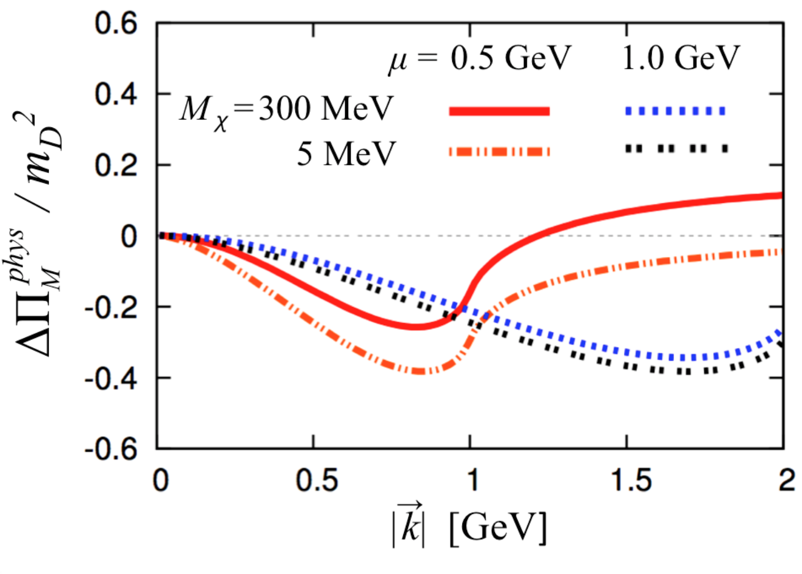
For the singlet phase we take the same parameter set as for the Higgs phase. Figure 9 shows the behavior of the polarization functions. The main differences from the normal and Higgs phases can be seen in the electric sector. The IR contributions are vanishing; in particular, for MeV, the electric contribution is well below that in the normal phase. The quark color density is much stiffer against color perturbations than in the normal phase, which implies that electric gluons in the IR region are unaffected by screening, unless is significantly enhanced in the infrared. The size of the unscreened domain is characterized by the size of the gap, shrinking as decreases.
The infrared behavior in the magnetic sector, is quite similar to that in the normal phase. While its behavior in the UV is different, it has little quantitative impact on the total, where vacuum contributions growing like become large.
Figure 10 also shows comparisons of the various contributions. The electric sector is well dominated by particle-hole contributions; in the magnetic sector, the situation is similar to that in the normal phase. The particle-hole and particle-antiparticle contributions almost cancel out, and the remaining contributions are gauge-variant artifacts. We conclude that the in-medium gluons in the singlet phase behave in the infrared as vacuum gluons.


VII Summary and discussions
In this paper we have compared color screening in the normal, Higgs, and singlet phases. We studied the singlet phase using the example of two-color QCD with a color-singlet condensates near the Fermi surface. The presence of the gap provides qualitative differences among these phases. In particular, in the singlet phase both the electric and magnetic screening masses disappear, implying that soft gluons are protected from medium effects, as long as the quark-gluon vertex is not singular in the infrared.
An obvious question concerns the three-color version of the singlet phase. With two colors, the natural singlet condensate is a uniform diquark condensate. In contrast, in three-color QCD the diquark is colored, so we have to look for alternative condensates to carry over our arguments here. The usual uniform chiral condensate formed by particle-antiparticle pairs is not favored in the presence of a quark Fermi sea; instead one might imagine a uniform particle-hole condensate, but the allowed phase space is too small to favor such a condensate. In fact the usual gap equation for uniform chiral condensation at finite density automatically includes this possibility but does not yield a nontrivial solution.
One possible candidate would be a nonuniform chiral condensate made of particles and holes. The structure of the gap equation is like that in the BCS one, and the size of the gap can be enhanced by the quasi-low dimensionality near the Fermi surface. If gluons remain strongly interacting at densities of interest, the gap can be ; such a large gap can protect soft gluons from medium effects as discussed here, giving a self-consistent picture. In this context, studies of the non-uniform chiral condensates deserve further investigation.
Strong interactions of gluons—were they to remain up to GeV or larger—would justify a number of tacit assumptions in frequently employed effective-model calculations, e.g., the Nambu-Jona-Lasinio model. Effective models are usually formulated to describe the hadron phenomenology, incorporating gluon dynamics into a set of model parameters or particular forms of interactions, which can in principle change if the underlying gluon dynamics changes in the medium. The presence of condensates that forbid significant modifications in gluon dynamics would render such effective-model treatments consistent at finite density. Furthermore, the infrared protection of soft gluons would leave the gluon condensate—which is related to the QCD vacuum energy density—essentially unchanged. In this picture, the quark matter equation of state would not contain an additional constant term, e.g., a “bag constant.”
Another issue is the treatment of strange quarks. It is generally assumed that the strange quarks do not play a role until becomes close to the strange-quark effective mass, MeV. But the origin of the effective quark mass—chiral symmetry breaking— would disappear or significantly decrease once soft gluons are strongly screened; then a strange-quark Fermi sea would be formed much earlier than one would expect with a phenomenological strange-quark constituent mass, because the strange-quark current mass, MeV, is well below the typical scale for quark matter formation, MeV. The role of such an early onset of strange quarks in reducing the stiffness of the quark matter has been explored in Ref. [22].
Finally we compare the present one-loop considerations with lattice results for two-color QCD, which have studied the Landau-gauge gluon propagator in the presence of a color-singlet diquark condensate [11]. The lattice results, indicate that both electric and magnetic gluons in the infrared region are screened by medium effects, and look like gluons in the Higgs phase 99 9 This description may be misleading because a number of studies have indicated that the confined and Higgs phases can be smoothly connected [20, 21]. Indications are based on gauge-invariant correlation functions in which quarks and gluons are not separately discussed and all excitations are composite, with no color charges. Such a connection between the two phases is obscured in gauge-fixed computations using quark and gluon propagators, as here.. These results are most likely nonperturbative—with, as one expects, screening masses of order or —and cannot be interpreted within our present perturbative framework. Although our results have quantitative ambiguities, most of the present qualitative conclusions have been derived from considerations of phase-space restrictions introduced by the gaps. Thus we do not expect that the simple inclusion of higher-order loops to resolve the difference with the lattice calculations. Rather this discrepancy serves as a clue for deeper understanding of nonperturbative gluon dynamics that is not included in our computations.
Acknowledgments
This research was supported in part by NSF Grants PHY09-69790 and PHY13-05891. GB wishes to thank the RIKEN iTHES project for partial support.
Appendix A Derivation of the Ward-Takahashi identity
In this appendix we use the standard path-integral formalism to derive the generalized identity (38) from which follows the Ward-Takahashi identities used in Sec. III.3. Consider
| (109) |
where we write compactly
To derive the needed identities we change the integration variables for quarks, writing . This change of variables preserves the functional measure, and does not affect the expectation values resulting from integration. With the corresponding change of variables for the charge-conjugated fields, the Nambu-Gor’kov bases in the new and old variables are related as
| (110) |
with given by Eq. (12). The action, however, is not invariant under these changes of variables; using the relations , , and the resulting relation , we find the additional contribution
Since the change of integration variables does not affect the expectation value , the collection of terms linear in must sum to zero. Writing the change of as , we find the identity:
| (114) |
from which we derive several relations. For example, for , we find the quantum equation of motion, . Setting , we find Eq.(38).
References
- [1] J. C. Collins and M. J. Perry, Phys. Rev. Lett. 34 (1975) 1353.
- [2] B. A. Freedman and L. D. McLerran, Phys. Rev. D 16 (1977) 1130; ibid. 16 (1977) 1147; ibid. 16 (1977) 1169; V. Baluni, Phys. Lett. B 72 (1978) 381; ibid. Phys. Rev. D 17 (1978) 2092; A. Kurkela, P. Romatschke and A. Vuorinen, Phys. Rev. D 81 (2010) 105021 [arXiv:0912.1856 [hep-ph]].
- [3] M. G. Alford, A. Schmitt, K. Rajagopal and T. Schfer, Rev. Mod. Phys. 80 (2008) 1455 [arXiv:0709.4635 [hep-ph]].
- [4] D. H. Rischke, Phys. Rev. D 62 (2000) 034007 [nucl-th/0001040]; ibid. 054017 [nucl-th/0003063]; ibid. 64 (2001) 094003 [nucl-th/0103050];
- [5] K. Iida and G. Baym, Phys. Rev. D 65 (2002) 014022 [hep-ph/0108149]; M. Huang and I. A. Shovkovy, Phys. Rev. D 70 (2004) 051501 [hep-ph/0407049]; ibid. 094030 [hep-ph/0408268]; K. Fukushima, Phys. Rev. D 72 (2005) 074002 [hep-ph/0506080].
- [6] D. T. Son, Phys. Rev. D 59 (1999) 094019 [hep-ph/9812287].
- [7] Y. Nambu, Phys. Rev. 117 (1960) 648.
- [8] G. Baym and L. P. Kadanoff, Phys. Rev. 124 (1961) 287; G. Baym, Phys. Rev. 127 (1962) 1391.
- [9] A. Nakamura, Phys. Lett. B 149 (1984) 391.
- [10] J. B. Kogut, D. K. Sinclair, S. J. Hands and S. E. Morrison, Phys. Rev. D 64 (2001) 094505 [hep-lat/0105026]; J. B. Kogut, D. Toublan and D. K. Sinclair, Phys. Lett. B 514 (2001) 77 [hep-lat/0104010]; S. Hands, J. B. Kogut, M. -P. Lombardo and S. E. Morrison, Nucl. Phys. B 558 (1999) 327 [hep-lat/9902034]. J. B. Kogut, D. K. Sinclair, S. J. Hands and S. E. Morrison, Phys. Rev. D 64 (2001) 094505 [hep-lat/0105026].
- [11] T. Boz, S. Cotter, L. Fister, D. Mehta and J. -I. Skullerud, Eur. Phys. J. A 49 (2013) 87 [arXiv:1303.3223 [hep-lat]]; S. Cotter, P. Giudice, S. Hands and J. -I. Skullerud, Phys. Rev. D 87 (2013) 3, 034507 [arXiv:1210.4496 [hep-lat]]. S. Hands, P. Kenny, S. Kim and J. -I. Skullerud, Eur. Phys. J. A 47 (2011) 60 [arXiv:1101.4961 [hep-lat]]. S. Hands, S. Kim and J. -I. Skullerud, Phys. Rev. D 81 (2010) 091502 [arXiv:1001.1682 [hep-lat]]; ibid., Eur. Phys. J. C 48 (2006) 193 [hep-lat/0604004].
- [12] G. Baym, H. Monien, C. J. Pethick and D. G. Ravenhall, Phys. Rev. Lett. 64 (1990) 1867.
- [13] L. McLerran and R. D. Pisarski, Nucl. Phys. A 796 (2007) 83 [arXiv:0706.2191 [hep-ph]].
- [14] A. B. Migdal, Rev. Mod. Phys. 50 (1978) 107; R. F. Sawyer, Phys. Rev. Lett. 29 (1972) 382; R. F. Sawyer and D. J. Scalapino, Phys. Rev. D 7 (1973) 953; G. Baym, Phys. Rev. Lett. 30 (1973) 1340.
- [15] D. V. Deryagin, D. Y. .Grigoriev and V. A. Rubakov, Int. J. Mod. Phys. A 7 (1992) 659; E. Shuster and D. T. Son, Nucl. Phys. B 573 (2000) 434 [hep-ph/9905448]; B. -Y. Park, M. Rho, A. Wirzba and I. Zahed, Phys. Rev. D 62 (2000) 034015 [hep-ph/9910347]; R. Rapp, E. V. Shuryak and I. Zahed, Phys. Rev. D 63 (2001) 034008 [hep-ph/0008207]; E. Nakano and T. Tatsumi, Phys. Rev. D 71 (2005) 114006 [hep-ph/0411350].
- [16] D. Nickel, Phys. Rev. D 80 (2009) 074025; S. Carignano, D. Nickel and M. Buballa, Phys. Rev. D 82 (2010) 054009 [arXiv:1007.1397 [hep-ph]]; D. Mller, M. Buballa and J. Wambach, Phys. Lett. B 727 (2013) 240 [arXiv:1308.4303 [hep-ph]].
- [17] T. Kojo, Y. Hidaka, L. McLerran and R. D. Pisarski, Nucl. Phys. A 843 (2010) 37 [arXiv:0912.3800 [hep-ph]]; T. Kojo, R. D. Pisarski and A. M. Tsvelik, Phys. Rev. D 82 (2010) 074015 [arXiv:1007.0248 [hep-ph]]; T. Kojo, Y. Hidaka, K. Fukushima, L. D. McLerran and R. D. Pisarski, Nucl. Phys. A 875 (2012) 94 [arXiv:1107.2124 [hep-ph]].
- [18] D. H. Rischke, D. T. Son and M. A. Stephanov, Phys. Rev. Lett. 87 (2001) 062001 [hep-ph/0011379].
- [19] R. D. Pisarski and D. H. Rischke, Phys. Rev. D 60 (1999) 094013 [nucl-th/9903023].
- [20] E. H. Fradkin and S. H. Shenker, Phys. Rev. D 19 (1979) 3682.
- [21] J. Greensite, Prog. Part. Nucl. Phys. 51 (2003) 1 [hep-lat/0301023].
- [22] P. D. Powell and G. Baym, Phys. Rev. D 88, 014012 (2013).