What do precision Higgs measurements buy us?
Abstract
We study the sensitivities of future precision Higgs measurements and electroweak observables in probing physics beyond the Standard Model. Using effective field theory—appropriate since precision measurements are indirect probes of new physics—we examine two well-motivated test cases. One is a tree-level example due to a singlet scalar field that enables the first-order electroweak phase transition for baryogenesis. The other is a one-loop example due to scalar top in the MSSM. We find both Higgs and electroweak measurements are sensitive probes of these cases.
For decades, experimental efforts have chased the Higgs boson like the holy grail while, at the same time, theoretical pursuits have tried to make sense of all of its unnatural and mysterious features. Having discovered a “Higgs boson” [1, 2], these unnatural and mysterious features immediately become pressing questions. Models of new physics address these questions by making the Higgs more natural if we can avoid a finely-tuned cancellation between the bare parameter and the quadratic divergence in its mass-sqaured and less mysterious if we can explain why there is only one scalar in the theory and what dynamics causes it to condense in the Universe.
Obviously we need to study this new particle as precisely as we can, which calls for an collider such as ILC or a circular machine (TLEP/CEPC). ILC has been through an intensive internatinonal study through six-year-long Global Design Effort that released the Technical Design Report in 2013 [3, *Baer:2013cma, *Adolphsen:2013jya, *Adolphsen:2013kya, *Behnke:2013lya]. Given the technical readiness, we hope to understand the fiscal readiness in the next few years. The studies on a very high intensity circular machine have just started [8].
In the past, precision measurements using electrons revealed the next important energy scale and justified the next big machine. The polarized electron-deuteron scattering at SLAC measured the weak neutral currents precisely [9], which led to the justification of SpS and LEP colliders to study bosons. The precision measurements at SLC/LEP predicted the mass of the top quark [10] and the Higgs boson [11], which were verified at the Tevatron [12, 13] and LHC [1, 2], respectively. We hope that precision measurements of the Higgs boson will again point the way to a definite energy scale.
In this letter, we study what precision Higgs measurements may tell us for two very different new physics scenarios. One is a singlet scalar coupled to the Higgs boson, where impacts arise at the tree level. It can achieve first-order electroweak phase transition which would allow electroweak baryogenesis. The other is the scalar top in the Minimal Supersymmetric Standard Model (MSSM), where impacts arise at the one-loop level. It will help minimize the fine-tuning in the Higgs mass-squared. In both cases, we find the sensitivities of future precision Higgs and precision electroweak measurements are similar.
I The Standard Model effective field theory
Precision physics programs offer indirect probes of new physics, thereby neccesitating a model-independent framework to analyze potential patterns of deviation from known physics. This framework is most naturally formulated in the language of an effective field theory (EFT) which, for our interests, consists of the Standard Model (SM) supplemented with higher-dimension interactions,
| (1) |
In the above, is the cutoff scale of the EFT, are dimension operators that respect the gauge invariance of , and are their Wilson coefficients. In the following, we loosely use the term Wilson coefficient to refer to either or the operator coefficient, . The meaning is clear from context.
Effective field theories are arguably the most appropriate framework for studying the indirect probes of a precision program. However, we need to know just how big do we expect the Wilson coefficients to be in well-motivated models of beyond the Standard Model (BSM) physics. To shed light on this question, for the models studied in this letter we first integrate out heavy states and obtain the Wilson coefficients of the generated higher-dimension operators and then relate these coefficients to measurable Higgs observables.
In practice, due to suppression by the high scale , the irrelevant operators kept in the EFT are truncated at some dimension. The estimated per mille sensitivity of future precision Higgs programs, together with the present lack of evidence of BSM physics coupled to the SM, justifies keeping only the lowest dimension operators in the effective theory. In the SM effective theory this includes a single dimension-five operator that generates neutrino masses (that we henceforth ignore) and dimension-six operators.
There is a caveat in interpreting Wilson coefficients as the inverse of heavy particle masses if BSM states couple directly to the Higgs. The Wilson coefficients in Eq. (1) are computed with mass parameters in the Lagrangian, while the actual mass eigenvalues receive additional contribution from the Higgs vev and mixings. This difference is accounted for by higher-dimension operators which are dropped in our analysis. Therefore, the experimental sensitivities on Wilson coefficients do not translate directly into those on heavy particle masses. We will quantify this difference in each example.
We now turn our attention to the dimension-six operators relevant for our analysis. Since many of the most sensitive probes of Higgs properties involve only bosons, we restrict our attention to the purely bosonic dimension-six operators listed in Table 1. Some of these operators are redundant because they can be rewritten by other dimension-six operators using the SM equations of motion (e.g. ) [14, 15]. We maintain these so-called redundant operators in our analysis because (1) their impact on physical observables remains most transparent and (2) they are directly generated using standard techniques of integrating out heavy states. While the relationship between some of these operators and physical observables can be found in the literature (e.g. [16, 17, 18, 19, 20]), we provide elsewhere the complete mapping between the operators in Table 1 and physical observables as well as techniques for obtaining their Wilson coefficients from UV models [21].
Over the past year there has been much progress on understanding the SM EFT and its relation to Higgs physics. We briefly comment on some of these developments (see [20] for a recent review). A common theme is the basis of operators in the effective theory; a complete basis of dimension-six operators contains 59 operators [15]. The choice of this basis is not unique; however, maintaining a complete basis is crucial for consistent treatment of renormalization group (RG) evolution within the EFT [22]. Several different bases are common in the literature [15, 23, 24] (see [20] for comparison), and even these are often slightly tweaked [16, 17]. Our choice of operators in Table 1 coincides with [17], supplemented by the operators and . After specifying a (potentially overcomplete) basis, the Wilson coefficients can be mapped onto physical observables [20, 16, 17, 18, 19, 21]. An overcomplete basis containing redundant operators may also be used, although the RG evolution requires some care [22, 16, 17]. Global fits and constraints on the size of Wilson coefficients in the EFT have also been analyzed [18, 16, 17, 25, *Mebane:2013zga, *Mebane:2013cra].
II A massive singlet
We consider a heavy gauge singlet that couples to the SM via a Higgs portal
| (2) | |||||
There are several motivations for studying this singlet model. This single additional degree of freedom can successfully achieve a strongly first-order electroweak phase transition (EWPT) [28]. Additionally, singlet sectors of the above form—with particular relations among the couplings—arise in the NMSSM [29] and its variants, e.g. [30, 31]. Finally, the effects of Higgs portal operators are captured through the trilinear and quartic interactions and , respectively.
For the singlet can be integrated out; at tree level the resultant low-energy theory contains a finite correction to the Higgs potential as well as the operators and :
| (3) |
Upon electroweak symmetry breaking, modifies the wavefunction of the physical Higgs and therefore universally modifies all the Higgs couplings,
| (4) |
where . This universal Higgs oblique correction can be quite sensitive to new physics [35, 36, 37] since future lepton colliders, such as the ILC, can probe it at the per mille level [38]. In Fig. 1, we show the contour of this oblique correction. The contour is obtained by combining the future expected sensitivities of Higgs couplings across all 7 channels in Table 1-20 of [38] for an ILC 500up program, except for the channel where we used the updated value provided by the second column in Table 6 of [39]. As shown, the ILC is quite sensitive to this oblique correction, exploring masses up to several TeV and much of the parameter space of the singlet’s couplings to the SM.
In addition to the oblique correction, will generate measurable contributions to electroweak precision observables (EWPO) under renormalization group evolution. The anomalous dimension matrix characterizes the RG mixing amongst dimension-six operators in the SM EFT from a UV scale to the weak scale ,
| (5) |
The anomalous dimension matrix has been recently computed [16, 17, 22, 40, 19]. We use the results of [17]. 11 1 We note that the work [17] calculates within a complete operator basis even though they provide only a subset of the full anomalous dimension matrix. Further, upon changing bases, the results of [17] agree with another recent computation of the full anomalous dimension matrix [22, 40, 19].
Of the EWPO, we find the and parameters to be the most constraining; in terms of the operators in Table 1 the and parameters are given by
| (6) | ||||
| (7) |
where . RG evolution of generates the operators and with anomalous dimension coefficients [17]
| (8) |
For the singlet model at hand,
| (9) | ||||
| (10) |
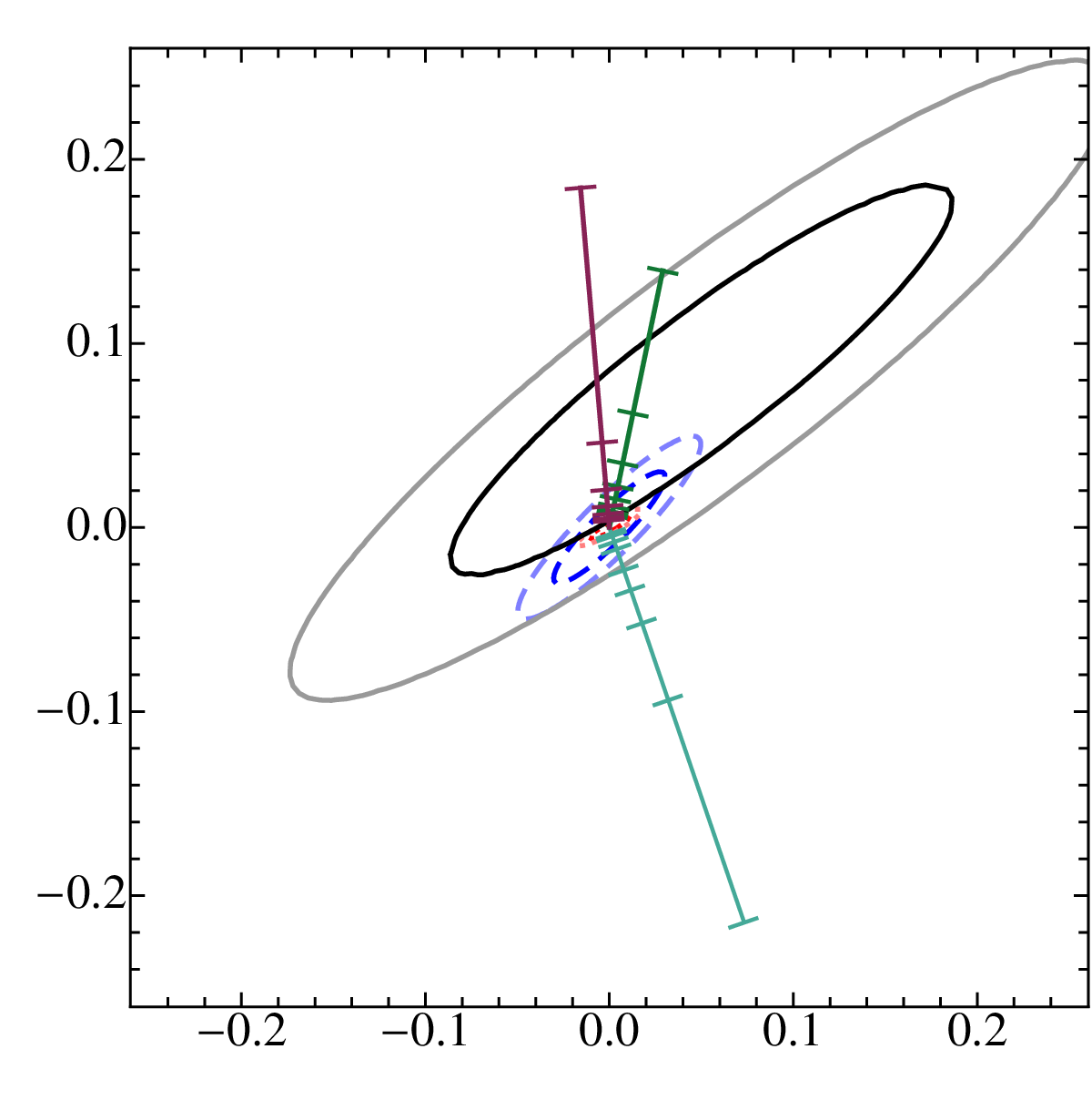
It is worth noting that and are highly correlated—current fits find a correlation coefficient of [32]—while the RG evolution of generates and in the orthogonal direction of this correlation, as depicted in Fig. 3. This orthogonality feature enhances the sensitivity of EWPO to oblique Higgs corrections, even when the new physics does not directly couple to the EW sector.
The current best fit of the and parameters are [32]
| (11) |
This precision is already sensitive to potential next-to-leading order physics which typically comes with a loop suppresion, as in our singlet model. Future lepton colliders will significantly increase the precision measurements of and ; a GigaZ program at the ILC would increase precision to [4, 33] while a TeraZ program at TLEP estimates precision of [8, 34]. Constraints on our singlet model from current and prospective future lepton collider measurements of and are shown in Fig. 1. As seen in the figure, the combination of increased precision measurements together with the fact that the singlet generates and in the anti-correlated direction, makes these EWPO a particularly sensitive probe of the singlet. Note that the apparent lack of improvement by GigaZ is an artifact of current non-zero central values in and .
As previously mentioned, this simple singlet model can achieve a strongly first-order EW phase transition. Essentially, this occurs by having a negative quartic Higgs coupling while stabalizing the potential with ,
for positive coeffiecients . Within a thermal mass approximation,22 2 A full one-loop calculation at finite temperature does not drastically alter the bounds in Eq. (12); the lower bound remains the same, while the upper bound is numerically raised by about 25% [41]. This region is still well probed by future lepton colliders. a first-order EWPT occurs when [28]
| (12) |
where we have set for simplicity. The lower bound comes from requiring EW symmetry breaking at zero temperature, while the upper bound comes from requiring , which guarantees the phase transition is first order.
The region of viability for a strongly first-order EWPT within the singlet model is shown in Fig. 1, for nominal values of the coupling (note that has an upper limit of from perturbativity and lower limit from stability). Current EWPO already constrain a substantial fraction of the viable parameter space, while future lepton colliders will probe the entire parameter space.
Finally, we comment on the accuracy of the present calculation. Upon EW symmetry breaking, , the singlet gains an additional contribution to its mass-squared of order and mixes with . The light eigenstate of this mixing is the physical Higgs with mass 125 GeV. As discussed earlier, these effects make the mass eigenvalue of the heavy scalar differ from the inverse of the Wilson coefficient in the effective Lagrangian Eq. (3). The difference is of the order of
We note that this difference is very small over most of the region shown in Fig. 1.
III Light scalar tops
As a second benchmark scenario, we consider the MSSM with light scalar tops (stops) and examine the low energy EFT resultant from integrating out these states. Stops hold a priviledged position in alleviating the naturalness problem, e.g. [42]. This motivates us to consider a spectrum with light stops while other supersymmetric partners are decoupled. Since the stops carry all SM gauge quantum numbers, all of the dimension-six operators in Table 1 are generated at leading order (1-loop). Therefore, they also serve as an excellent computational example to estimate the parametric size of Wilson coefficients of the operators in Table 1 resultant from heavy scalar particles with SM quantum numbers. Since the Wilson coefficients are generated at 1-loop leading order, we discard, as an approximation, the relatively smaller RG running effects (2-loop) of the Wilson coefficients.

When we integrate out the multiplet , we take degenerate soft masses for simplicity. We computed the Wilson coefficients using a covariant derivative expansion [47, 48, 21] and checked them against standard Feynman diagram techniques. The resultant Wilson coefficients are listed in Table 2, where and .
As in the previously considered singlet model, these Wilson coefficients will correct Higgs widths universally through Eq. (4), as well as contribute to and parameters through Eq. (6)-(7). In contrast to the singlet case, the stops contribute to both the oblique correction (via ) and EWPOs (via , , and ) at leading order (1-loop). Additionally, vertex corrections to and decay widths—arising from , , , and —are sensitive probes since these are loop-level processes within the SM. The deviations from the SM decay rates are given by
| (13) | |||||
where and are the standard form factors in their respective SM decay rates (see, e.g., [49]).
sensitivity contours are shown in Fig. 2. We stress that here we are focused on the experimental sensitivities on the scalar top mass, while assuming improvements on relevant theoretical uncertainties will catch up in time. Analogous to the case of the singlet model, in the plot differs from the mass eigenvalue by about . As seen in Fig. 2, future precision Higgs and EW measurements from the ILC offer comparable sensitivities while a TeraZ program significantly increases sensitivity. Moreover, the most natural region of the MSSM—where and (e.g. [50])—can be well probed by future precision measurements.
Acknowledgements.
This work was supported by the U.S. DOE under Contract DE-AC03-76SF00098, by the NSF under grants PHY-1002399 and PHY-1316783. HM was also supported by the JSPS grant (C) 23540289, and by WPI, MEXT, Japan.References
- [1] G. Aad et al. (ATLAS Collaboration), Phys.Lett. B716, 1 (2012), arXiv:1207.7214 [hep-ex] .
- [2] S. Chatrchyan et al. (CMS Collaboration), Phys.Lett. B716, 30 (2012), arXiv:1207.7235 [hep-ex] .
- [3] T. Behnke, J. E. Brau, B. Foster, J. Fuster, M. Harrison, et al., (2013a), arXiv:1306.6327 [physics.acc-ph] .
- [4] H. Baer, T. Barklow, K. Fujii, Y. Gao, A. Hoang, et al., (2013), arXiv:1306.6352 [hep-ph] .
- [5] C. Adolphsen, M. Barone, B. Barish, K. Buesser, P. Burrows, et al., (2013a), arXiv:1306.6353 [physics.acc-ph] .
- [6] C. Adolphsen, M. Barone, B. Barish, K. Buesser, P. Burrows, et al., (2013b), arXiv:1306.6328 [physics.acc-ph] .
- [7] T. Behnke, J. E. Brau, P. N. Burrows, J. Fuster, M. Peskin, et al., (2013b), arXiv:1306.6329 [physics.ins-det] .
- [8] M. Bicer et al. (TLEP Design Study Working Group), JHEP 1401, 164 (2014), arXiv:1308.6176 [hep-ex] .
- [9] C. Prescott, W. Atwood, R. L. Cottrell, H. DeStaebler, E. L. Garwin, et al., Phys.Lett. B84, 524 (1979).
- [10] G. Alexander et al. (LEP Collaborations, ALEPH Collaboration, DELPHI Collaboration, L3 Collaboration, OPAL Collaboration), Phys.Lett. B276, 247 (1992).
- [11] S. Schael et al. (ALEPH Collaboration, DELPHI Collaboration, L3 Collaboration, OPAL Collaboration, SLD Collaboration, LEP Electroweak Working Group, SLD Electroweak Group, SLD Heavy Flavour Group), Phys.Rept. 427, 257 (2006), arXiv:hep-ex/0509008 [hep-ex] .
- [12] F. Abe et al. (CDF Collaboration), Phys.Rev.Lett. 74, 2626 (1995), arXiv:hep-ex/9503002 [hep-ex] .
- [13] S. Abachi et al. (D0 Collaboration), Phys.Rev.Lett. 74, 2632 (1995), arXiv:hep-ex/9503003 [hep-ex] .
- [14] W. Buchmuller and D. Wyler, Nucl.Phys. B268, 621 (1986).
- [15] B. Grzadkowski, M. Iskrzynski, M. Misiak, and J. Rosiek, JHEP 1010, 085 (2010), arXiv:1008.4884 [hep-ph] .
- [16] J. Elias-Miro, J. Espinosa, E. Masso, and A. Pomarol, JHEP 1311, 066 (2013a), arXiv:1308.1879 [hep-ph] .
- [17] J. Elias-Miro, C. Grojean, R. S. Gupta, and D. Marzocca, (2013b), arXiv:1312.2928 [hep-ph] .
- [18] A. Pomarol and F. Riva, JHEP 1401, 151 (2014), arXiv:1308.2803 [hep-ph] .
- [19] R. Alonso, E. E. Jenkins, A. V. Manohar, and M. Trott, (2013), arXiv:1312.2014 [hep-ph] .
- [20] S. Willenbrock and C. Zhang, (2014), arXiv:1401.0470 [hep-ph] .
- [21] B. Henning, X. Lu, and H. Murayama, In preparation.
- [22] E. E. Jenkins, A. V. Manohar, and M. Trott, JHEP 1310, 087 (2013), arXiv:1308.2627 [hep-ph] .
- [23] G. Giudice, C. Grojean, A. Pomarol, and R. Rattazzi, JHEP 0706, 045 (2007), arXiv:hep-ph/0703164 [hep-ph] .
- [24] K. Hagiwara, S. Ishihara, R. Szalapski, and D. Zeppenfeld, Phys.Rev. D48, 2182 (1993).
- [25] C.-Y. Chen, S. Dawson, and C. Zhang, Phys.Rev. D89, 015016 (2014), arXiv:1311.3107 [hep-ph] .
- [26] H. Mebane, N. Greiner, C. Zhang, and S. Willenbrock, Phys.Rev. D88, 015028 (2013a), arXiv:1306.3380 [hep-ph] .
- [27] H. Mebane, N. Greiner, C. Zhang, and S. Willenbrock, Phys.Lett. B724, 259 (2013b), arXiv:1304.1789 [hep-ph] .
- [28] C. Grojean, G. Servant, and J. D. Wells, Phys.Rev. D71, 036001 (2005), arXiv:hep-ph/0407019 [hep-ph] .
- [29] J. R. Ellis, J. Gunion, H. E. Haber, L. Roszkowski, and F. Zwirner, Phys.Rev. D39, 844 (1989).
- [30] X. Lu, H. Murayama, J. T. Ruderman, and K. Tobioka, (2013), arXiv:1308.0792 [hep-ph] .
- [31] R. Barbieri, L. J. Hall, Y. Nomura, and V. S. Rychkov, Phys.Rev. D75, 035007 (2007), arXiv:hep-ph/0607332 [hep-ph] .
- [32] M. Baak, M. Goebel, J. Haller, A. Hoecker, D. Kennedy, et al., Eur.Phys.J. C72, 2205 (2012), arXiv:1209.2716 [hep-ph] .
- [33] M. Baak, A. Blondel, A. Bodek, R. Caputo, T. Corbett, et al., (2013), arXiv:1310.6708 [hep-ph] .
- [34] S. Mishima, “Talk given at the Sixth TLEP Workshop,” (2013).
- [35] N. Craig, C. Englert, and M. McCullough, Phys.Rev.Lett. 111, 121803 (2013), arXiv:1305.5251 [hep-ph] .
- [36] C. Englert and M. McCullough, JHEP 1307, 168 (2013), arXiv:1303.1526 [hep-ph] .
- [37] S. Gori and I. Low, JHEP 1309, 151 (2013), arXiv:1307.0496 [hep-ph] .
- [38] S. Dawson, A. Gritsan, H. Logan, J. Qian, C. Tully, et al., (2013), arXiv:1310.8361 [hep-ex] .
- [39] M. E. Peskin, (2013), arXiv:1312.4974 [hep-ph] .
- [40] E. E. Jenkins, A. V. Manohar, and M. Trott, JHEP 1401, 035 (2014), arXiv:1310.4838 [hep-ph] .
- [41] C. Delaunay, C. Grojean, and J. D. Wells, JHEP 0804, 029 (2008), arXiv:0711.2511 [hep-ph] .
- [42] M. Papucci, J. T. Ruderman, and A. Weiler, JHEP 1209, 035 (2012), arXiv:1110.6926 [hep-ph] .
- [43] S. Heinemeyer, W. Hollik, and G. Weiglein, Comput.Phys.Commun. 124, 76 (2000), arXiv:hep-ph/9812320 [hep-ph] .
- [44] S. Heinemeyer, W. Hollik, and G. Weiglein, Eur.Phys.J. C9, 343 (1999), arXiv:hep-ph/9812472 [hep-ph] .
- [45] G. Degrassi, S. Heinemeyer, W. Hollik, P. Slavich, and G. Weiglein, Eur.Phys.J. C28, 133 (2003), arXiv:hep-ph/0212020 [hep-ph] .
- [46] M. Frank, T. Hahn, S. Heinemeyer, W. Hollik, H. Rzehak, et al., JHEP 0702, 047 (2007), arXiv:hep-ph/0611326 [hep-ph] .
- [47] M. Gaillard, Nucl.Phys. B268, 669 (1986).
- [48] O. Cheyette, Nucl.Phys. B297, 183 (1988).
- [49] A. Djouadi, Phys.Rept. 457, 1 (2008), arXiv:hep-ph/0503172 [hep-ph] .
- [50] L. J. Hall, D. Pinner, and J. T. Ruderman, JHEP 1204, 131 (2012), arXiv:1112.2703 [hep-ph] .