Binary pattern tile set synthesis is NP-hard
Abstract
In the field of algorithmic self-assembly, a long-standing unproven conjecture has been that of the -hardness of binary pattern tile set synthesis (2-Pats). The -Pats problem is that of designing a tile assembly system with the smallest number of tile types which will self-assemble an input pattern of colors. Of both theoretical and practical significance, -Pats has been studied in a series of papers which have shown -Pats to be -hard for , , and then . In this paper, we close the fundamental conjecture that -Pats is -hard, concluding this line of study.
While most of our proof relies on standard mathematical proof techniques, one crucial lemma makes use of a computer-assisted proof, which is a relatively novel but increasingly utilized paradigm for deriving proofs for complex mathematical problems. This tool is especially powerful for attacking combinatorial problems, as exemplified by the proof of the four color theorem by Appel and Haken (simplified later by Robertson, Sanders, Seymour, and Thomas) or the recent important advance on the Erdős discrepancy problem by Konev and Lisitsa using computer programs. We utilize a massively parallel algorithm and thus turn an otherwise intractable portion of our proof into a program which requires approximately a year of computation time, bringing the use of computer-assisted proofs to a new scale. We fully detail the algorithm employed by our code, and make the code freely available online.
1 Introduction
Self-assembly is the process through which disorganized, relatively simple components autonomously coalesce according to simple local rules to form more complex target structures. Despite sounding simple, self-assembly can produce extraordinary results. For example, and beyond the many examples occurring in nature, researchers have been able to self-assemble a wide variety of nanoscale structures experimentally, such as regular arrays [43], fractal structures [33, 10], smiley faces [32, 41], DNA tweezers [45], logic circuits [35, 28], neural networks [29], and molecular robots[22]. These examples are fundamental because they demonstrate that self-assembly can, in principle, be used to manufacture specialized geometrical, mechanical and computational objects at the nanoscale. Potential future applications of nanoscale self-assembly include the production of new materials with specifically tailored properties (electronic, photonic, etc.) and medical technologies which are capable of diagnosing and even treating diseases in vivo and at the cellular level.
Controlling nanoscale self-assembly for the purposes of manufacturing atomically precise components will require a bottom-up, hands-off strategy. In other words, the self-assembling units themselves will have to be “programmed” to direct themselves to assemble efficiently and correctly. Molecular self-assembly is rapidly becoming a ubiquitous engineering paradigm, and robust theory is necessary to inform us of its algorithmic capabilities and ultimate limitations.
In 1998, Erik Winfree [42] introduced the abstract Tile Assembly Model (aTAM), a simplified discrete mathematical model of algorithmic DNA nanoscale self-assembly pioneered by Seeman [36]. The aTAM is essentially an asynchronous nondeterministic cellular automaton that models crystal growth processes. Put another way, the aTAM augments classical Wang tiling [40] with a mechanism for sequential growth of a tiling. This contrasts with classical Wang tiling in which only the existence of a valid mismatch-free tiling is considered, and not the order of tile placement. In the aTAM, the fundamental components are translatable but un-rotatable square tiles whose sides are labeled with colored glues, each with an integer strength. Two tiles that are placed next to each other interact if the glue colors on their abutting sides match, and they bind if the strengths on their abutting sides match and sum to at least a certain (integer) temperature. Self-assembly starts from an initial seed assembly and proceeds nondeterministically and asynchronously as tiles bind to the seed-containing-assembly. Despite its deliberate simplification, the aTAM is a computationally expressive model in which simulations of arbitrary Turing computations have been built [42] and complex series of computations performed [27, 20]. It has even been shown recently to be intrinsically universal [8, 9, 7, 25, 44, 6].
The problem we study in this paper is the optimization of the design of tile assembly systems in the aTAM which self-assemble to form input colored patterns. The input for this problem is a rectangular pattern consisting of colors, and the output is a tile set in the aTAM which self-assembles the pattern. Essentially, each type of tile is assigned a “color”, and the goal is to design a system consisting of the minimal number of tile types such that they deterministically self-assemble to form a rectangular assembly in which each tile is assigned the same color as the corresponding location in the pattern. This problem was introduced in [23], and has since then been extensively studied [11, 21, 5, 37, 17, 16]. The interest is both theoretical, to determine the computational complexity of designing efficient tile assembly systems, and practical, as the goal of self-assembling patterned substrates onto which a potentially wide variety of molecular components could be attached is a major experimental goal. Known as -Pats, where is the number of unique colors in the input pattern, previous work has steadily decreased the value of for which -Pats has been shown to be -hard, from [37] to [17] to [16]. (Additionally, in a variant of -Pats where the number of tile types of certain colors is restricted, is has been proven to be -hard for colors [18].) However, the foundational and previously unproven conjecture has been that for , i.e. -Pats, the problem is also -hard. This is our main result, which is thus the terminus of this line of research and a fundamental result in algorithmic self-assembly.
Our proof of the -Pats conjecture requires the solution of a massive combinatorial problem, and thus one of the lemmas upon which it relies has a computer-assisted proof. That is, it relies upon the output of a computer program which exhaustively searches through a combinatorially explosive set of all possible tile sets which can self-assemble a particular, carefully designed input pattern. (In fact, during each run our, verification program generated over partial tile assemblies to be inspected.) Although not yet commonplace in theoretical results, computer-assisted proofs are becoming more widespread, driven by the exponential growth of computing power which can be applied to previously and otherwise intractable problems. Nonetheless, as early as 1976, Appel and Haken proved the four color theorem [2, 3] by using a computer program to check whether each of the thousands of possible candidates for the smallest-sized counter example to this theorem were actually four-colorable or not (simplified in [31]). Since then, important problems in various fields have been solved (fully or partially) with the assistance of computers: the discovery of Mersenne primes [39], the 17-point case of the happy ending problem [38], the -hardness of minimum-weight triangulation [26], a special case of Erdős’ discrepancy conjecture [19], the ternary Goldbach conjecture [14], and Kepler’s conjecture [13, 24], among others. However, to the best of our knowledge, the scale of our computation is much greater than all of those and others which have been published. Our program required approximately one year of computation time on very modern, high-end machines (as a sum total over several hundred distributed cores) to complete and verify the correctness of the lemma. Thus, in this paper, we take this approach to a new order of magnitude. Such techniques create new possibilities, spanning beyond the aesthetic concerns usually associated with the domain (see quotations from Paul Erdős in [15]). Indeed, our proof takes several days to complete on a massively parallel computer, which makes it essentially impossible for a human to verify. This kind of method is likely to become common when it comes to proving correctness of biological or chemical systems, due to the complexity of these objects. Moreover, the “natural proofs” line of research [30, 34, 1, 4] also suggests that our ability to produce and verify large proofs is likely to become fundamental in complexity theory.
The computer program that we used in our proof was written in C++, and we have made the code freely available online11 1 http://self-assembly.net/wiki/index.php?title=2PATS-tileset-search. Furthermore, we provide a full technical description and justification of the main algorithm utilized by the code in Section 4. 22 2 We have also implemented the same algorithm in a client-server system written in Haskell and included a rigorous proof of its correctness as the appendix, since as a functional programming language Haskell lends itself more readily to formal proofs of program correctness. However, at the time of submission, due to decreased efficiencies as compared to C++, the Haskell program has not yet completed.
1.1 Main result
Our result solves a long-standing open problem in the field of DNA self-assembly, the so-called binary pattern tile set synthesis (2-Pats) problem [23, 37]. In the general -Pats for , given a placement of different kinds of nanoparticles, represented in the model as a -colored rectangular pattern, we are asked to design a tile assembly system with colored tile types that self-assembles the pattern. The periodic placement of Au (gold) nanoparticles on 2D DNA nanogrid [46] can be considered a 2-colored (i.e., binary) rectangular pattern on which the two colors specify the presence/absence of an Au nanoparticle at the position. Another example, shown in Figure 1, is a binary counter pattern that is self-assembled using 4 tile types with two colors. 2-Pats has been conjectured to be -hard33 3 This problem was claimed to be so in the succeeding paper by the authors of [23] but what they proved was the NP-hardness of a related but different problem.. In [37], Seki proved for the first time that the -hardness of 60-Pats, whose inputs are allowed to have 60 colors, and the result has been strengthened to that of 29-Pats [17], and further to that of 11-Pats [16] recently.
Our main theorem closes this line of research by lowering the number of colors allowed for input patterns to only two. Although a number of terms it contains have not yet been defined, we state it now:
Theorem 1.
The -Pats optimization problem of finding, given a colored rectangular pattern , the minimal colored tileset that produces a single terminal assembly where the color arrangement is exactly the same as in , is NP-hard.
1.2 Overview of our proof technique
The main idea of our proof is similar to the strategies adopted by [37, 17, 16]. We embed the computation of a verifier of solutions for an NP-complete problem (in our case, a variant of Sat, which we call M-Sat) in an assembly, which is relatively straightforward in Winfree’s aTAM. One can indeed engineer a tile assembly system (TAS) in this model, with colored tiles, implementing a verifier of solutions of the variant of Sat, in which a formula and a variable assignment are encoded in the seed assembly, and a tile of a special color appears after some time if and only if . In our actual proof, reported in Section 3, we design a set of 13 tile types and a reduction of a given instance of M-Sat to a rectangular pattern such that
- Property 1.
A TAS using tile types in self-assembles if and only if is satisfiable.
- Property 2.
Any TAS of at most 13 tile types that self-assembles is isomorphic to .
Therefore, is solvable if and only if can be self-assembled using at most 13 tile types. In previous works [37, 17, 16], significant portions of the proofs were dedicated to ensuring their analog of Property 2, and many colors were wasted to make the property “manually” checkable (for reference, 33 out of 60 colors just served this purpose for the proof of -hardness of 60-Pats [37] and 2 out of 11 did that for 11-Pats [16]). Cutting this “waste” causes a combinatorial explosion of cases to test and motivates us to use a computer program to do the verification instead.
Apart from the verification of Property 2 (in Lemma 3), the rest of our proof can be verified as done in traditional mathematical proofs; our proof is in Section 3. The verification of Property 2 is done by an algorithm described in Section 4.2, which, given a pattern and an integer , searches exhaustively for all possible sets of tile types that self-assemble the pattern. The correctness of the algorithm is proven, and the C++ code implementing the algorithm is made freely available for inspection.
2 Preliminaries
This section is divided into three subsections: necessary notions and notation on rectilinear tile assembly system, definitions related to the Pats problem, and then a preliminary lemma about the variant of Sat that we use.
2.1 Pattern assembly
Let be the set of nonnegative integers, and for , let . For , a -colored pattern is a partial function from to the set of (color) indices , and a -colored rectangular pattern (of width and height ) is a pattern whose domain is .


Let be a glue alphabet. A (colored) tile type is a tuple , where represent the respective north, west, south, and east glue of , and is a color (index) of . For instance, the right black tile type in Figure 1 (Left) is (1, 1, 0, 0, black). We refer to as , respectively, and by we denote the color of . For a set of tile types, an assembly over is a partial function from to . (When algorithms and computer programs will be explained in Section 4, it is convenient for the tile types in to be indexed as and consider the assembly rather as a partial function to .) Its pattern, denoted by , is such that and for any . Given another assembly , we say is a subassembly of if and, for any , .
A rectilinear tile assembly system (RTAS) is a pair of a set of tile types and an L-shape seed , which is an assembly over another set of tile types disjoint from such that for some . Its size is measured by the number of tile types employed, that is, . According to the following general rule all RTASs obey, it tiles the first quadrant delimited by the seed:
RTAS’s tiling rule: To a given assembly , a tile can attach at position if
- 1.
is undefined,
- 2.
both and are defined,
- 3.
and .
The attachment results in a larger assembly whose domain is such that for any , , and . When this attachment takes place in the RTAS , we write . Informally speaking, the tile can attach to the assembly at if on , both and are tiled while is not yet, and the west and south glues of match the east glue of the tile at and the north glue of the tile at , respectively. This implies that, at the outset, (0, 0) is the sole position where a tile may attach.
For those who are familiar with the Winfree’s aTAM [42], it should be straightforward that an RTAS is a temperature-2 tile assembly system all of whose glues are of strength 1.
Example 2.
See Figure 1 for an RTAS with 4 tile types, aiming at self-assembling the binary counter pattern. To its L-shape seed shown there, a black tile of type (1, 1, 0, 0, black) can attach at (0, 0), while no tile of other types can due to glue mismatches. The attachment makes the two positions (0, 1) and (1, 0) attachable. Tiling in RTASs thus proceeds from south-west to north-east rectilinearly until no attachable position is left.
The set of producible assemblies by is defined recursively as follows: (1) , and (2) for , if , then . A producible assembly is called terminal if there is no assembly such that . The set of terminal assemblies is denoted by . Note that the domain of any producible assembly is a subset of , starting from the seed whose domain is .
A tile set is directed if for any distinct tile types , or holds. An RTAS is directed if its tile set is directed (the directedness of RTAS was originally defined in a different but equivalent way). It is clear from the RTAS tiling rule that if is directed, then it has the exactly one terminal assembly, which we let . Let be the subassembly of the terminal assembly such that , that is, the tiles on did not originate from the seed but were tiled by the RTAS. Then we say that uniquely self-assembles the pattern .
2.2 The Pats problem
The pattern self-assembly tile set synthesis (Pats), proposed by Ma and Lombardi [23], aims at computing the minimum size directed RTAS that uniquely self-assembles a given rectangular pattern. The solution to Pats is required to be directed here, but not originally. However, in [12], it was proved that among all the RTASs that uniquely self-assemble the pattern, the minimum one is directed.
To study the algorithmic complexity of this problem on “real size” particle placement problems, a first restriction that can be placed is on the number of colors allowed for the input patterns, thereby defining the -Pats problem:
Problem (-colored Pats (-Pats)).
-
Given: A -colored pattern ;
-
Output: a smallest directed RTAS that uniquely self-assembles .
The NP-hardness of -Pats follows from the -hardness of its decision variant.
Problem (decision variant of -Pats).
-
Given: A -colored pattern and an integer ;
-
Output: “yes” if can be uniquely self-assembled by an RTAS whose tileset contains at most tile types.
In the rest of this paper, we use the terminology -Pats to refer to the decision problem, unless otherwise noted.
2.3 Monotone Satisfiability Problem
We now prove the -completeness of a modified version of Sat, which we will use in our proof. In the monotone satisfiability with few true variables (M-Sat), we consider a number and a boolean formula in conjunctive normal form without negations and ask whether or not can be satisfied by only allowing variables to be true.
Note that formulae with no negations are easily satisfied by setting all the variables to .
Lemma 1.
M-Sat is -complete.
Proof.
First, for any formula and assignment of its variables, it can be checked in polynomial time that . Therefore, M-Sat is in . -hardness follows from an easy reduction from Vertex Cover: let be a graph, and for any , let and be two variables, and be the clause defined by . Finding an assignment with a minimal number of true variables in is then equivalent to finding a minimal vertex cover of . ∎
3 2-Pats is -hard
We will prove that Pats is -hard for binary patterns (-colored patterns). First, we present a binary gadget pattern such that among all tilesets of size at most , exactly one self-assembles . Let be this tileset.
Then, we present a reduction from M-Sat to the problem of deciding whether an input pattern can be assembled with . The -hardness of 2-Pats follows, since we ensure that the input pattern contains the gadget pattern as a subpattern, hence forcing the use of to assemble .
The reduction is proved in Theorem 1, and the claim that it is the only tileset of size at most 13 that can assemble is proved in Lemma 3, using a programmatic proof. is shown on Figure 2; it contains eleven white tile types and two black tile types.
We interpret the glues in the tile set as follows. Ten of the white tile types (first and second rows in Figure 2) simulate three types of signals which interact with each other:
- 1.
blue signals running from left to right,
- 2.
green signals running from bottom to top, and
- 3.
red signals running diagonally from bottom left to top right in a wavelike line.
For better visibility in printouts the red signals are dotted; blue and green signals can easily be distinguished as blue signals run only horizontally while green signals run only vertically. When any two of the signals meet, they simply cross over each other, where the red signal is displaced upwards or rightwards when crossing a blue or green signal, respectively. Only when the blue signal crosses a green signal immediately before crossing a red signal, the red signal is destroyed. In order to recognize this configuration, the blue signal is tagged when it crosses a green signal; in Figure 2, the tagging is displayed by the fork in the blue signal. Let us stress that the signals are encoded in the glues of the tiles, they are not visible. The other three tile types are used to uncover the green and red signals in two consecutive rows: two black tiles above each other stand for no signal, a white tile below a black tile stands for a green signal, a black tile below a white tile stands for a red signal, and blue signals are never uncovered. Note that green (respectively, red) signals switch to red (respectively, green) in the first uncover row, but they switch back to their original state in the second uncover row. An example assembly is shown in Figure 3.
Clearly, the green signals always progress upwards from one glue to the next and blue signals progress rightwards from one glue to the next. Let us formalize the progression of the red signal under the assumption that it is not destroyed.
Lemma 2.
Let the south glue of a tile in position be a red signal. If this red signal progresses up-/rightwards to the south glue of a tile in position while crossing green signals, and blue signals, and no uncovering rows, then
Proof.
In every row where the red signal crosses a blue signal, the red signal remains at its horizontal position. Thus, only in the rows without blue signal the red signal moves rightwards. In each of these rows, we move one positions rightwards plus one position for every green signal that is crossed on the total way. We conclude that . ∎
By using a computer-aided search through all tile assignments with 13 tile types of the pattern shown in Figure 4, we obtain the following lemma:
Lemma 3.
The gadget pattern , shown in Figure 4, can only be self-assembled with 13 tile types if a tile set is used which is isomorphic to . No smaller tile set can self-assemble .
Proof.
Details about the program that we used for the computer-aided search are presented in Section 4. ∎
In order to prove the -hardness of -Pats we encode an instance of M-Sat into the problem of deciding whether or not an initial configuration of red and green signals can be transformed into a target configuration of red and green signals after a certain number of steps. The clue is that the hidden positions of blue signals refer to variables which are true in a satisfying variable assignment of the M-Sat instance.
Theorem 1.
-Pats is -hard.
Proof.
Let and be a set of clauses which is an instance of M-Sat. For convenience, we assume that is defined over the variables . We design a pattern based on and such that can be self-assembled with no more than tile types if and only if is satisfiable with only positive variables. The pattern , schematically presented in Figure 5, contains two rows defining the initial configuration and two rows containing the target configuration . These two rows are separated by completely white rows. The gadget pattern is attached in the top left corner of the pattern and is separated by 11 white rows from the target configuration. The area right of the gadget pattern is composed of the progression of the red and green signals which appear in the target configuration and where we consider the 11 white rows to have no blue signal and the signals in the following 24 rows are as required by the gadget pattern.
Since the target and initial configurations are represented by two rows of black or white pixels and cannot contain a pair of white pixels above each other, they can be interpreted as words over the three-letter alphabet , where stands for no signal, encodes a green signal, and encodes a red signal. The target and initial configuration rows are
where
encodes the green signals which appear in the gadget pattern; and for the -th clause in , the sequence contains pairs of black pixels and pixel pairs , which represent green signals, such that for variable we find a green signal in which is preceded by a total of black pixel pairs (and possibly some green signals) in :
(for a sequence and a symbol , the integer equals the number of occurrences of in ignoring all other symbols in ). Note that the width of the pattern is in . The pattern can be computed from and in polynomial time. See Example 3 at the end of this section for the conversion of a short formula into a pattern.
Suppose that the pattern can be self-assembled with tile types. As includes the subpattern , we only have to focus on the question of whether or not can be self-assembled by the tile set , shown in Figure 2; see Lemma 3. Since we only have two black tile types in and these can only occur in an uncover row, it is clear that all tiles in and have the glue on all of their east and west edges, and that they are the only tiles with that glue on their east and west edges. Obviously, these three uncover tile types, uniquely define the assembly of the initial and target configuration. Also, the white uncover tile type cannot be used in any position in the white area between the initial and target configuration; otherwise, there had to be a complete white row with only this tile type which implied that all rows above had to have red signals as south input, and some of these red signals ultimately had to appear in the target configuration. Also the glue sequence on the south part of the seed is determined by .
Observe that the following sequence of vertical glues can be used as part of the west seed which lies above the target configuration from bottom to top
The first 11 glues in this sequence together with the green signals in form the south input of the gadget pattern , thusly, allowing the gadget pattern to self-assemble in the top left corner of . (This is because the pattern grows from the bottom left to the top right, and red signals which are input into the south of the gadget pattern grow diagonally up and right, starting from this sequence, with some of them moved further to the right when crossing green signals.)
After we showed that the part of the pattern which lies above the two rows can be self-assembled, we will prove that the lower part of the pattern up to and including the two rows can be self-assembled if and only if is satisfiable. Let the sequence denote the west glues in between the rows and from bottom to top. Note that this is the only part of the pattern that is not fixed yet; it will carry the information of how to choose the variable assignment in order to satisfy . We are interested only in the blue signals which are hidden in and we do not care about any red signals which might be included in ; hence, when convenient we assume where represents no signal or a red signal. Consider the sequence in which turns into in . Note that the red signal in , encoded by , is is the only red signal in the entire final configuration . Since there are no green signals encoded in and by Lemma 2, this red signal has to be initiated at most positions to the left in . Therefore, the origin of the red signal in is indeed the red signal encoded in . Furthermore, as this red signal moves by positions to the right from to , we conclude that exactly of the white rows contain a hidden blue signal, by Lemma 2.
Now, we will show that if is satisfiable, then the pattern can be self-assembled by . Let be a satisfying variable assignment for with . We let contain non-signal glues and for each variable with we add a blue signal in which is preceded by glues and possibly other blue signals:
Note that and that contains blue signals as variables have to be true in . Consider in which represents the clause . In this sequence turns into where all the green signals appear in the same positions, but the red signal does not appear anymore. Note that if this red signal in were not destroyed, then it had show up as the last pixel of in , by Lemma 2. As satisfies there is a variable with . By definition of , we have with and we have with . Suppose that the red signal does not get destroyed before it passes the green signal representing . After passing this green signal, the red signal has moved columns without signals to the right (the last of these columns lies right of the green signal), therefore, the signal also traveled rows without signals upwards and it has to cross the blue signal which corresponds to in the next step, see Figure 6. We see that the red signal is destroyed on the way from to , and hence, this sequence in can successfully be transformed into the corresponding sequence in . As this argument holds for every clause and we already showed how the remainder of the pattern can be self-assembled, we conclude that if is satisfiable with true variables, then can be self-assembled with tile types.
Vice versa, suppose can be self-assembled by the tile set and an appropriately chosen seed. We define a variable assignment based on the sequence of west glues , as defined above. We let if and only if there is a blue signal in which is preceded by glues (recall that, stands for everything other than a blue signal):
As there are blue signals in we have that the number of positive variable assignments in is at most . Due to the monotone nature of the formula (it does not contain negations), if we prove that can be satisfied with at most positive variables in the assignment, then can also be satisfied with exactly positive variables in the assignment. As we already observed above, the pixel sequence in which represents the clause is transformed into in , and hence, the red signal has to be destroyed within the white area of the pattern. Note that a blue signal in the first position of will not destroy the red signal as the red signal does not have a green signal as left neighbor. Thus, the red signal is destroyed when it hits one signal which stands for a positively assigned variable in . The green signal which is also involved in the destruction of the red signal is separated by black pixel pairs from the red signal in ; see Figure 6 again. The existence of this green signal implies that and the clause is satisfied by . We conclude that satisfies every clause in , and hence, itself. ∎
Example 3.
Figure 7 shows a tile assignment for the pattern which is generated from the formula with . The part of the pattern which is needed for the gadget attachment is ignored in this example.
4 Programmatic search for the minimal tile set
We present our algorithm for finding all tile sets of a given size which self-assemble a given -colored pattern on a rectangle (in our case and ). In Section 4.1, we show that it is sufficient to generate all valid tile assemblies for the given pattern, which use at most tile types, rather than generating all tile sets with all possible -shaped seeds. We present our algorithm which generates these valid tile assemblies and the corresponding tile sets in Section 4.2 and discuss several methods which we implemented to speed up the algorithm. Lastly, we discuss the parallel implementation and the performance of the algorithm in the two programming languages C++ (Section 4.3) and Haskell (Section 4.4).
4.1 RTASs defined by assemblies
Consider the -colored pattern . Recall that for a tile set a terminal assembly (without the seed structure) of is a mapping such that
- (a)
if , then for all and ,
- (b)
for all and , and
- (c)
for all and .
Condition (a) implies that every tile type can only have one color and conditions (b) and (c) ensure that there are no vertical or horizontal glue mismatches in the assembly. An (partial) assembly is a partial mapping which satisfies the three conditions for all positions which are defined in . Every RTAS that self-assembles yields a terminal assembly by enumerating the tiles in where the seed is implicitly constituted by the south glues of the tiles for and the west glues of the tiles for .
Conversely, every mapping which satisfies condition (a) yields a (not necessarily directed) tile set where condition (b) imposes equivalence classes on the vertical glues and condition (c) imposes equivalence classes on the horizontal glues (e.g. the glue belongs to the same equivalence class as the glue ). For each of these equivalence classes we reserve one unique glue label in ; in particular, no vertical glue gets the same label as a horizontal glue. Thus, is a terminal assembly of for . Next, we show that if is a terminal assembly of for a tile set , then is a morphic image of ; that is, there exists a bijection of tile types , and a morphisms from the glues of to the glues of such that for all and we have and . Let and be the chosen tile enumerations with respect to the assembly , then the bijection is chosen such that for all . Since both, and , have to satisfy (a), we obtain that as desired. Furthermore, was defined such that it satisfies the minimal requirements for to be an assignment according to conditions (b) and (c). Because must also satisfy these two conditions, it is clear that the morphism can be defined.
Note that the fact that is a morphic image of implies that if is a directed tile set, then is directed as well (though, the converse does not necessarily hold). Henceforth, we call an assembly valid if it is terminal and its corresponding tile set is directed. The algorithm that we present next lists all valid assemblies of together with their corresponding directed tile sets with at most tile types. Therefore, up to morphic images of these solution tile sets, it lists all directed tile sets which can self-assemble . Also note that if a directed tile set is a morphic image of our tile set shown in Fig. 2, then and are isomorphic. This can easily be verified as every tile set which is obtained by combining any two horizontal glues or any two vertical glues in is an undirected tile set.
4.2 The algorithm
Instead of fully generating every terminal assembly of the pattern and then checking whether or not the corresponding tile set is directed, we generate partial assemblies tile by tile while adapting a generic tile set in each step such that it satisfies conditions (a) through (c) from Section 4.1. If a tile set which corresponds to an assembly is not directed, then we do not have to place any further tiles into this assembly because any larger assembly which contains as subassembly has a corresponding undirected tile set and, hence, cannot be completed to become a valid assembly. This procedure can be illustrated in a tree spanning the search space where every node is a partial assembly with corresponding tile set. Its root is the empty assembly (no tiles are placed) whose corresponding tile set consists of tile types with every glue of every tile type unique and all tiles un-colored. Leaves in this tree are either solutions, valid assemblies of with a corresponding directed tile set, or breakpoints, nodes whose tile sets are not directed.
The tiles are placed according to a tile placing strategy; that is, each position in has a successor position where the next tile is placed. The correctness of the algorithm does not depend on the tile placing strategy, however, the performance of the algorithm highly depends on this strategy. Our strategy is to keep the area that is covered by tiles as compact as possible. Performance tests on small patterns confirmed that the average depth of paths in the tree spanning the search space is smaller when using our strategy as compared to the naive row-by-row or column-by-column approaches. The ordering of positions is illustrated in Fig. 8, and is intuitively defined by “the alternative addition of a row and a column”, starting as shown in the figure. Formally, this amounts to defining a sequence of coordinates inductively by and
The cases in the formula can be interpreted as follows, from top to bottom: start a new row, start a new column, add one tile to an existing column, add one tile to an existing row. This simplified formula suggests that the pattern has to be a square, but it can also be interpreted as ordering on all positions in the rectangular pattern by simply skipping positions which lie outside of .
Let be a partial assembly in which exactly the first positions, according to the tile placing strategy, are covered with tiles and let be the corresponding tile set which we assume to be directed. Therefore, can be viewed as a node in the tree spanning the search space which is not a leave. We try out all possible tile types in the empty position as follows:
- 1.
If there is a tile type in the current tile set which fits (i.e. its glues match those adjacent to the position and its color matches ), a tile of that type is placed in . Note that due to the ordering of tile placements, the adjacent glues (if any) will always be to the west and/or south, ensuring that those are the input sides. If the location is on the bottom (left) edge of the pattern, there will not be an input glue on the south (west).
- 2.
Else if, for each tile type which has already been placed somewhere in the assembly and which has color , the west and south glues of can be changed to match those adjacent to the current position, wherever they occur throughout the current tiles of the assembly (modifying additional tile types as necessary). If the tile set remains directed (i.e. no tile types have the same input glues), then the glue changes are made and is placed in the current location.
- 3.
Else, if the number of tile types which are used in the partial assembly are less than , change the glues of one unused type so that it matches those adjacent to the current location, assign the color , and place a tile of that type in position .
Note that this procedure is optimized such that it will not generate two assemblies which are permutations of each other because we do not try several unused tile types in the same position. The tree spanning the search space which is defined through this procedure is recursively traversed in a depth-first manner.
If this procedure finds a valid assignment of with a corresponding directed tile set , then we output as solution. As discussed in Section 4.1, this algorithm will output all directed tile sets which can self-assemble up to morphic images. Both, the Haskell and C++ version of our program, are parallelized implementations of the algorithm described here.
4.3 Implementation in C++
The C++ code uses MPI 44 4 The implementation is Open MPI: http://www.open-mpi.org as its communication protocol and a simple strategy for sharing the work among the cores. The master process generates a list containing all partial assemblies in which exactly 14 positions are covered by tiles and whose corresponding tile sets are directed. This list contains 271,835 partial assemblies, or jobs, in the case of our gadget pattern from Section 3. The master sends out one of these jobs to each of the client processes. Afterwards, the master process only gathers the results of jobs that were finished by clients and assigns new jobs to clients on request. When the list is empty the master sends a kill signal to each client process that requests a new job.
A client process which got assigned the partial assembly generates all valid assemblies of which contain as a subassembly with corresponding directed tile set, using the algorithm described in Section 4.2. When one job is finished, possible solutions are transmitted to the master and a new job is requested by the client. In this implementation we did not address the computational bottleneck that emerges when client processes finish the last jobs and then have to idle until the last client process is finished. There is no concept of sharing a job after it has been assigned to a client.
The C++ implementation of our algorithm55 5 Freely available for download here: http://self-assembly.net/wiki/index.php?title=2PATS-tileset-search was run on the cluster saw.sharcnet.ca of Sharcnet66 6 https://www.sharcnet.ca/my/systems/show/41. The cluster allowed us to utilize the processing power of 256 cores of Intel Xeon 2.83GHz (out of the total 2712 cores) for our computation. In order to minimize the chances of the already unlikely event that undetected network errors influenced the outcome of the computation, our program was run twice on this system, with both runs yielding the same result, namely that the tile set from Fig. 2 is the only tile set (up to isomorphism) with 13 or less tile types capable of generating the gadget pattern , thus proving Lemma 3. Each of the computations finished after almost 35 hours using a total CPU time of approximately 342 days. Note that this implies a combined CPU idle time of about 30 days for the clients which we assume to be chiefly caused by the computational bottleneck at the end of the computation. During one computation all the cores together generated over partial tile assemblies.
4.4 Implementation in Haskell
The kind of intensive proofs our approach uses has traditionally been proven “rigorously”, with consensual proofs, several years after their first publication. This means that some of the latest proofs rely on the simplicity of their implementation to make them checkable. Moreover, proof assistants like Coq are not yet able to provide a fast enough alternative, to verify really large proofs in a reasonable amount of time.
Things are beginning to change, however, and the gap between rigorous and algorithmic proofs is being progressively bridged. The ultimate goal of this research direction is to get rigorous proofs as the first proof of a theorem, even in the case of explorations run on large parallel computers.
In order to reach this goal for Lemma 3, we wrote a library to be used for additional algorithmic proofs whose size requires a parallel implementation. It also allows to work with different computing platforms, including grids, clusters and desktop computers.
This library, called Parry, is available at http://parry.lif.univ-mrs.fr. Its version 0.1, with SHA1 sum d572cbb7189d1d8232982913c70b3cfcb72ec44f, is rigorously proven in the appendix of this paper.
Remarkably enough for a parallel program, its proof makes no hypotheses on the network, and only relies on the equivalence of Haskell semantics and its compiled assembly version, as well as on the security of cryptographic primitives.
Unfortunately, this implementation is relatively slower than the C++ one described in section 4.3, and is still running at the time of submitting this paper.
5 Acknowledgements
We would like to thank Manuel Bertrand for his infinite patience and helpful assistance with setting up the server and helping debug our network and system problems. We also thank Cécile Barbier, Eric Fede and Kai Poutrain for their assistance with software setup.
References
- [1] E. Allender and M. Koucký. Amplifying lower bounds by means of self-reducibility. J. ACM, 57(3):14:1–14:36, Mar. 2010.
- [2] K. Appel and W. Haken. Every planar map is four colorable. Part I. discharging. Illinois Journal of Mathematics, 21:429–490, 1977.
- [3] K. Appel and W. Haken. Every planar map is four colorable. Part II. reducibility. Illinois Journal of Mathematics, 21:491–567, 1977.
- [4] T. Y. Chow. Almost-natural proofs. J. Comput. Syst. Sci., 77(4):728–737, July 2011.
- [5] E. Czeizler and A. Popa. Synthesizing minimal tile sets for complex patterns in the framework of patterned DNA self-assembly. In D. Stefanovic and A. Turberfield, editors, DNA Computing and Molecular Programming, volume 7433 of Lecture Notes in Computer Science, pages 58–72. Springer Berlin / Heidelberg, 2012.
- [6] E. D. Demaine, M. L. Demaine, S. P. Fekete, M. J. Patitz, R. T. Schweller, A. Winslow, and D. Woods. One tile to rule them all: simulating any Turing machine, tile assembly system, or tiling system with a single puzzle piece. Technical report, 2012. Arxiv preprint: arXiv:1212.4756.
- [7] E. D. Demaine, M. J. Patitz, T. A. Rogers, R. T. Schweller, S. M. Summers, and D. Woods. The two-handed tile assembly model is not intrinsically universal. In ICALP: 40th International Colloquium on Automata, Languages and Programming, volume 7965 of LNCS, pages 400–412, Riga, Latvia, July 2013. Springer. Arxiv preprint: arXiv:1306.6710.
- [8] D. Doty, J. H. Lutz, M. J. Patitz, R. T. Schweller, S. M. Summers, and D. Woods. The tile assembly model is intrinsically universal. In Proceedings of the 53rd Annual IEEE Symposium on Foundations of Computer Science, pages 439–446, Oct. 2012. Arxiv preprint: arXiv:1111.3097.
- [9] D. Doty, J. H. Lutz, M. J. Patitz, S. M. Summers, and D. Woods. Intrinsic universality in self-assembly. In Proceedings of the 27th International Symposium on Theoretical Aspects of Computer Science, pages 275–286, 2009. Arxiv preprint: arXiv:1001.0208.
- [10] K. Fujibayashi, R. Hariadi, S. H. Park, E. Winfree, and S. Murata. Toward reliable algorithmic self-assembly of DNA tiles: A fixed-width cellular automaton pattern. Nano Letters, 8(7):1791–1797, 2007.
- [11] M. Göös and P. Orponen. Synthesizing minimal tile sets for patterned DNA self-assembly. In DNA, pages 71–82, 2010.
- [12] M. Göös and P. Orponen. Synthesizing minimal tile sets for patterned DNA self-assembly. In DNA16: Proceedings of the 16th International Conference on DNA Computing and Molecular Programming, volume 6518 of LNCS, pages 71–82. Springer, 2011.
- [13] T. C. Hales. Cannonballs and honeycombs. Notices of the AMS, 47(4):440–449, 2000.
- [14] H. A. Helfgott. The ternary Goldbach conjecture is true. 2013.
- [15] P. Hoffman. The Man Who Loved Only Numbers: The Story of Paul Erdös and the Search for Mathematical Truth. Hyperion, New York, 1998.
- [16] A. Johnsen, M.-Y. Kao, and S. Seki. A manually-checkable proof for the NP-hardness of 11-colored patterned self-assembly of tile set synthesis. In preparation.
- [17] A. Johnsen, M. Y. Kao, and S. Seki. Computing minimum tile sets to self-assemble color patterns. In ISAAC 2013: Proceedings of the 24th International Symposium on Algorithms and Computation, volume 8283 of LNCS, pages 699–710. Springer, 2013.
- [18] L. Kari, S. Kopecki, and S. Seki. 3-color bounded patterned self-assembly. In DNA Computing and Molecular Programming, pages 105–117. Springer, 2013.
- [19] B. Konev and A. Lisitsa. A SAT attack on the Erdös discrepancy conjecture. arXiv: 1402.2184, 2014.
- [20] J. I. Lathrop, J. H. Lutz, M. J. Patitz, and S. M. Summers. Computability and complexity in self-assembly. Theory Comput. Syst., 48(3):617–647, 2011.
- [21] T. Lempiäinen, E. Czeizler, and P. Orponen. Synthesizing small and reliable tile sets for patterned DNA self-assembly. In Proceedings of the 17th international conference on DNA computing and molecular programming, DNA’11, pages 145–159, Berlin, Heidelberg, 2011. Springer-Verlag.
- [22] K. Lund, A. T. Manzo, N. Dabby, N. Micholotti, A. Johnson-Buck, J. Nangreave, S. Taylor, R. Pei, M. N. Stojanovic, N. G. Walter, E. Winfree, and H. Yan. Molecular robots guided by prescriptive landscapes. Nature, 465:206–210, 2010.
- [23] X. Ma and F. Lombardi. Synthesis of tile sets for DNA self-assembly. IEEE T. Comput. Aid. D., 27(5):963–967, 2008.
- [24] C. Marchal. Study of the Kepler’s conjecture: The problem of the closest packing. Mathematische Zeitschrift, 267(3-4):737–765, 2011.
- [25] P.-E. Meunier, M. J. Patitz, S. M. Summers, G. Theyssier, A. Winslow, and D. Woods. Intrinsic universality in tile self-assembly requires cooperation. In Proceedings of the 25th Annual ACM-SIAM Symposium on Discrete Algorithms (SODA), pages 752–771, 2014. Arxiv preprint: arXiv:1304.1679.
- [26] W. Mulzer and G. Rote. Minimum-weight triangulation is NP-hard. Journal of the ACM, 55(2):Article No. 11, 2008.
- [27] M. J. Patitz and S. M. Summers. Self-assembly of decidable sets. Natural Computing, 10(2):853–877, 2011.
- [28] L. Qian and E. Winfree. Scaling up digital circuit computation with DNA strand displacement cascades. Science, 332(6034):1196, 2011.
- [29] L. Qian, E. Winfree, and J. Bruck. Neural network computation with DNA strand displacement cascades. Nature, 475(7356):368–372, 2011.
- [30] A. A. Razborov and S. Rudich. Natural proofs. In Proceedings of the Twenty-sixth Annual ACM Symposium on Theory of Computing, STOC ’94, pages 204–213, New York, NY, USA, 1994. ACM.
- [31] N. Robertson, D. P. Sanders, P. Seymour, and R. Thomas. A new proof of the four-colour theorem. Electronic Research Announcements of the American Mathematical Society, 2(1):17–25, 1996.
- [32] P. W. Rothemund. Folding DNA to create nanoscale shapes and patterns. Nature, 440(7082):297–302, 2006.
- [33] P. W. Rothemund, N. Papadakis, and E. Winfree. Algorithmic self-assembly of DNA Sierpinski triangles. PLoS Biology, 2(12):2041–2053, 2004.
- [34] S. Rudich. Super-bits, demi-bits, and NP/qpoly-natural proofs. Journal of Computer and System Sciences, 55:204–213, 1997.
- [35] G. Seelig, D. Soloveichik, D. Y. Zhang, and E. Winfree. Enzyme-free nucleic acid logic circuits. Science, 314(5805):1585–1588, 2006.
- [36] N. C. Seeman. Nucleic-acid junctions and lattices. Journal of Theoretical Biology, 99:237–247, 1982.
- [37] S. Seki. Combinatorial optimization in pattern assembly (extended abstract). In UCNC 2013: Proceedings of the Unconventional Computation and Natural Computation - 12th International Conference, volume 7956 of LNCS, pages 220–231. Springer, 2013.
- [38] G. Szekeres and L. Peters. Computer solution to the 17-point Erdös-Szekeres problem. The ANZIAM Journal, 48:151–164, 2006.
- [39] B. Tuckerman. The 24th Mersenne prime. Proceedings of the National Academy of Sciences, 68:2319–2320, 1971.
- [40] H. Wang. Proving theorems by pattern recognition – II. The Bell System Technical Journal, XL(1):1–41, 1961.
- [41] B. Wei, M. Dai, and P. Yin. Complex shapes self-assembled from single-stranded DNA tiles. Nature, 485(7400):623–626, 2012.
- [42] E. Winfree. Algorithmic Self-Assembly of DNA. PhD thesis, California Institute of Technology, June 1998.
- [43] E. Winfree, F. Liu, L. A. Wenzler, and N. C. Seeman. Design and self-assembly of two-dimensional DNA crystals. Nature, 394(6693):539–44, 1998.
- [44] D. Woods. Intrinsic universality and the computational power of self-assembly. 2013. Arxiv preprint: arXiv:1309.1265.
- [45] B. Yurke, A. J. Turberfield, A. P. Mills, F. C. Simmel, and J. L. Neumann. A DNA-fuelled molecular machine made of DNA. Nature, 406(6796):605–608, 2000.
- [46] J. Zhang, Y. Liu, Y. Ke, and H. Yan. Periodic square-like gold nanoparticle arrays templated by self-assembled 2D DNA nanogrids on a surface. Nano Letters, 6(2):248–251, 2006.
We now discuss the Haskell implementation of the proof of Lemma 3, and give a proof of this implementation.
Appendix A Global overview of the architecture
Our system is composed of two main components, a “server” and a “client”. The server orchestrates the work done by a collection of clients by assigning jobs (where a job is a current tile set and partial assembly) to each, monitoring their progress, and recording all discovered solutions. The clients are assigned jobs by the server and perform the actual testing of all possible tile sets within the fixed size bound (i.e. tile types) to see if they can self-assemble the input pattern. To prove the correctness of the system, we will individually prove the correctness of the server and client. The main result to be proven for the system is the following:
Lemma 4.
The server completes its search if and only if all tilesets of size (up to isomorphism) which can self-assemble the input pattern have been discovered.
The task of the server is to assign and keep track of all jobs which are being explored by the clients. Each client connects to it to ask for a job assignment. The server then replies with an assignment and keeps track of that job in case the client crashes, in which case the server will be able to detect that (in a way to be discussed) and reassign the job to another client. Along with that job, the server sends a boolean indicating whether it expects the job to be re-shared.
The clients’ messages to the server can be of three kinds: “get job” messages, new jobs (in our case, new tilesets and new partial assemblies to be explored), or a “job done” message, to tell the server that the job has been completed.
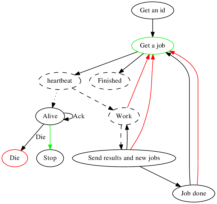
Formally, we can represent all possible states of the clients with the graph of Figure 9. In this figure, nodes drawn in solid lines represent states in which the client sends a message to the server, and edges represent state transitions of the client based on messages received from the server. Red edges are followed when the server sends an unexpected message (which is normally a “re-share” message, or one caused by the detection of an attacker), or when thread enters the “Die” red state. Dashed nodes and edges are “silent” client states and transitions, where no messages are sent or received.
Finally, the “heartbeat” state causes the creation of thread , and the “Die” and “Stop” states cause that thread to terminate. The green transition on that thread (from the “Alive” state to the “Stop” state) is triggered whenever thread enters the “Get job” state. The heartbeat thread otherwise exists in the “Alive” state. Both in the case of the green and red states, synchronization mechanisms ensure that the corresponding colored edges are followed in the other thread before the node is exited.
Appendix B The implementation
Our strategy to prove the whole system is the following:
The reason for this organization is to make the proof for the server and client reusable in other applications. We begin by defining what we mean by tasks, and how they can be represented in the server in an efficient way (by jobs).
Definition 4.
Let and be two sets, and be any function. A task is an element , and a result is an element . If there is a , and a set such that , we call the subtasks of .
We say that a task has been explored when is known.
In our code, most tasks are computed by computing their subtasks. For performance reasons, we cannot simply represent tasks in a direct way, and we need “jobs” instead:
Definition 5.
Let be a set (of tasks), be a set of results, and be any function. For any set , we say that is represented by if there is an onto map . In this case, for any , we say that is a job representation of .
By extension, for any job representing some task , jobs representing the subtasks of are called subjobs of .
B.1 How to read the code, and what we prove on it
The language we used to implement this architecture is the functional language Haskell. Although the syntax of this language may be somewhat surprising at first, the essential points that make our program easier to read, and easy to prove, are:
- •
Our program makes only one use of mutable variables, in the server’s global state. This is necessary to synchronize state variables between different threads.
All other variables that we use are non-mutable, meaning that new variables are created whenever a change is needed. For instance, in the client’s placeTile function, we will see in Section B.5 that new vectors are allocated when we need to change them.
- •
Global mutable variables are not allowed by the grammar and types of Haskell, hence all our functions depend on their arguments only (and, of course, on global constants).
- •
The type of functions tells whether or not they have side effects: a function has side effects (that is, modifies one of its arguments, or sends a message on the network) if and only if its type ends with “IO a” for some a (for example “IO ()”).
- •
Surprisingly, we do not need to prove anything about the messages sent by the server: any message sent by the protocol can be interpreted as a full predicate, sufficient to build a part of the global proof.
This makes the following kind of attacks possible: an attacker intercepts a “job mission” sent to a client and changes it. The client then starts to work on that job. However, when it sends “predicates” back to the server, these parts of the proof cannot be used, because they do not correspond to any “proof goal” in the server.
- •
Parts of this paper were generated directly from actual Haskell code using tools for literate programming. Therefore, the line numbers are actual line numbers, and might not be contiguous, in particular if some lines contain annotations for literate programming.
Moreover, many details of our functions need not be proven. In fact the only thing we need to prove is that the server does not halt before exploring all the tilesets it needs to explore.
In particular, we will not prove the efficiency or complexity of our protocol, nor the fact that the server will eventually halt on all runs: the fact that it halts on at least one run is sufficient for Lemma 3 to hold.
B.2 Protocol datatypes
We need to introduce a few datatypes to represent results, jobs, and client and server messages. Only representations of ClientMessage and ServerMessage via the encode function, along with signed hashes, will be passed on the network.
The first module we need is Parry.Protocol, that defines the type of messages exchanged between the client and server. We assume, in the rest of the proof, that the encode and decode functions generated by the Binary instances of these datatypes verify decode.encode is the identity.
15module Parry.Protocol where
16import Data.Binary
17import GHC.Generics (Generic)
18import Codec.Crypto.RSA.Pure
19
20-- | The type of messages sent by the client, exposed here for full
21-- disclosure of the protocol’s proof.
22data ClientMessage j=
23GetJob Integer PublicKey
24 JobDone { clientId::Integer, jobResults::[j], currentJob::j }
25 NewJobs { clientId::Integer, jobResults::[j], currentJob::j,
26nextJob::j, newJobs::[j] }
27 Alive Integer
28deriving (Generic, Show)
29
30-- | The type of messages sent by the server, exposed here for full
31-- disclosure of the protocol’s proof.
32data ServerMessage j=
33Job Bool j
34 Finished
35 Ack
36 Die
37deriving (Generic,Show)
38
39instance (Binary j)Binary (ClientMessage j)
40instance (Binary j)Binary (ServerMessage j)
B.3 Proof of the server
A good way to think of this code is the following: we are trying to build a giant proof tree, so big that no memory or even hard drive can handle it all. However, we can construct it “lazily” and in parallel, and at the same time verify it. This is why all the messages sent and received, that modify the server’s state, can be thought of as parts of the proof, of the form “I, valid client, hereby RSA-certify that the following is a valid part of the tree”.
The design of the protocol is such that every message that modifies the server’s state contains a complete predicate (for instance “the results in job j are exactly r”, or “While exploring j’s subjobs, I found results r, and the remaining subjobs are ”. The server’s task is then to assemble these predicates, which are summaries of subtrees of the proof, into a complete proof.
We now proceed to the proof of the server. The file is included for the sake of completeness. In particular, remark that the whole state of the server is defined as a single data type called State. We will use this fact to prove invariants on the whole server state.
25module Parry.Server (
26-- * Jobs on the server side
27Exhaustive(..),
28Result(..),
29-- * Server’s internal state
30initState,
31stateFromFile,
32saveThread,
33State(..),
34-- * Server configuration and functions
35Config(..),defaultConfig,server
36) where
37import Control.Concurrent
38import Control.Exception as E
39import Control.Monad
40import Control.Concurrent.MSem as Sem
41import Network
42import System.IO
43import System.Directory
44import Data.List
45import Data.Time.Format()
46import Data.Time.Clock.POSIX
47#ifdef UNIX
48import System.Posix.Signals
49#endif
50
51import qualified Data.ByteString.Char8 as B
52import qualified Data.ByteString.Lazy.Char8 as LB
53import qualified Data.Map as M
54import qualified Data.Set as S
55import GHC.Generics
56import Data.Binary
57
58import Codec.Crypto.RSA.Pure
59
60import Parry.Protocol
61import Parry.Util
62
63-- | The class of jobs and job results that Parry can deal with. For
64-- efficiency and to keep types simple, jobs and results are stored in
65-- a single type.
66class Exhaustive j where
67-- | Indication of the depth of a job in the explored tree. The server sends
68-- the least deep jobs first, as an optimization of network use.
69depth :: jInt
70-- | Number of times a job has been killed. When a job is killed,
71-- either because it must be reshared, or because the client itself
72-- was killed, it is scheduled to be re-executed by the server.
73killed::jInt
74-- | Called each time a job needs to be killed. For better resharing,
75-- this function must verify @killed (kill j) >= killed j@.
76kill::jj
77
78-- | The class of results, and how to combine them in the server state.
79class Result j r where
80-- | A function to tell how to combine job results. That function will be
81-- called on the hostname of the reporting client, with the finished job it
82-- sent, and the current result from the server state.
83addResult::HostNamerjr
84
85-- | This type is exposed mostly for writing alternative user interfaces.
86-- Other operations must be done using the functions in this module, or
87-- the correction of the protocol can be lost.
88data State j r=State {
89-- | Available jobs
90jobs::S.Set (Int,j),
91-- | Map from the machine id to its hostname, its current job, its
92-- starting time, the last time we heard from it.
93ongoing::M.Map Integer (HostName,PublicKey,j,Double,Double),
94-- | Set of unemployed machines
95unemployed::S.Set Integer,
96-- | The results.
97results::r,
98-- | The smallest available machine id. In a run of the server, it
99-- is guaranteed that are never assigned the same.
100newId::Integer,
101-- | Total number of jobs killed from the beginning (for benchmarking purposes).
102killings::Int,
103-- | Number of jobs finished (for benchmarking purposes).
104solved::Integer,
105-- | The list of authorized RSA public keys.
106authorizedKeys::[PublicKey]
107} deriving (Show,Read,Generic)
108
109instance (Binary j,Binary r)Binary (State j r)
Definition 6.
In a server state st, the current job of a client is the job registered in the ongoing field of st.
Definition 7.
We call a client valid if, at the same time:
- 1.
Its NewJobs messages contain all the results in subjobs of its current job that have been completely explored, and the subjobs of its current job that have not been completely explored, divided into three fields: the results it has found, its next current job, and other subjobs.
- 2.
It does not send a JobDone message before the task representing its current job is completely explored.
The main function, answer, keeps track of the clients. We now prove the following Lemma:
Lemma 5.
If st is a state of the server containing (in the union of job st and ongoing st) jobs representing all the tasks that have not yet been explored, and for any job j, j and kill j represent the same task, then for any message m sent by a valid client, all values of host and time, answer host time st m (the Haskell syntax for “the value of function answer, called with arguments t, host, st and m”) is a couple , where st’ is a state of the server containing the roots of all subtrees that have not yet been explored (m’ is the message to be sent to the client).
Moreover, all results sent by the clients are added to the server state using the addResult function.
Proof.
We prove it for all the cases.
118answer::(Exhaustive j,Result j r,Eq j,Ord j,Binary j)
119DoubleStringState j rClientMessage j
120(State j r,ServerMessage j)
121answer t host st (GetJob num key)=
122case M.lookup num (ongoing st) of
123Just (ho,key0,j0,t0,_)
If the client is registered as an “ongoing” job, we can simply send it the job it is supposed to be working on. In this case, the invariant is still maintained, as we do not change its recorded current job (here, we only update the time at which we last saw this client).
177if ho==host key0==key then
178(st { ongoing=M.insert num (ho,key,j0,t0,t) (ongoing st) },
179Job (not $ S.null $ unemployed st) j0)
180else
181(st,Die)
182Nothing
Else, client num is not in the map of ongoing jobs. If there are no more jobs to be done:
- •
if there are no more jobs being worked on, we do not modify the state, and we tell the client to stop (with a Finished message).
- •
else, we simply record that job as “unemployed”. The next time a client reports its state, it will be asked to share its current job. This does not change the jobs registered in the server’s state anyway.
189if S.null (jobs st) then
190if M.null (ongoing st) then
191(st,Finished)
192else
193(st { unemployed=S.insert num (unemployed st) },Die)
Else, if there are still jobs to be done, we pick any such job (using S.deleteFindMin). According to the documentation of Haskell’s Data.Map module, is equal to . Therefore, since num is not a member of ongoing st, the returned state contains, in the union of its ongoing and jobs fields, exactly the same jobs as in st.
207else
208let ((_,h),nextJobs)=S.deleteFindMin (jobs st)
209shareIt=killed h0
210in
211(st { jobs=nextJobs,
212unemployed=S.delete num (unemployed st),
213ongoing=M.insert num (host,key,h,t,t) (ongoing st) },
214Job shareIt h)
Another message the server can receive is the NewJobs message, when clients reshare their work: In this case, the client sends its number num, the initial job initialJob it was given, the new job job that it will now work on, a list js of jobs that need to be shared, and a list of results. We can think of this message as equivalent to “I, valid client num, hereby RSA-certify that job currentJob j you gave me has subjobs newJobs j, and results results j”.
223answer t host st j@(NewJobs {})=
224case M.lookup (clientId j) (ongoing st) of
225Nothing(st,Die)
226Just (ho,key,j0,t0,_)
227if host==ho j0==currentJob j then
228(st { jobs=foldl (s xS.insert (depth x,x) s) (jobs st) (newJobs j),
229ongoing=M.insert (clientId j)
230(host,key,nextJob j,t0,t)
231(ongoing st),
232results=foldl (addResult host) (results st) (jobResults j) }, Ack)
233else
234(st, Die)
If the client is not registered as an “ongoing job”, this message is ignored, the state is not modified, and the client is sent the Die message.
Else, we assumed that this NewJobs message can only be sent by a valid client. Therefore, it contains all subjobs of its current job that have not been explored, along with the job it will start working on, and the list of all results that have been found during the exploration of the other subjobs of its current job. Since all these subjobs are stored in the jobs field of the state, and the ongoing field is updated with the client’s new current job, our claim still holds.
247answer _ _ st j@(JobDone {})=
248case M.lookup (clientId j) (ongoing st) of
249Nothing(st,Die);
250Just (host,_,j0,_,_)
251if j0==currentJob j then
252(st { ongoing=M.delete (clientId j) (ongoing st),
253results=foldl (addResult host) (results st) (jobResults j),
254solved=solved st+1 }, Ack)
255else
256(st,Die)
In this case, if the client is not registered as an ongoing job, we do not modify the state. Else, we can safely delete the corresponding job from the state, and add its results to the state’s results field: indeed, since we assumed that this message is sent by a valid client, that job has been explored completely. The intuitive version of this message is “I, valid client num, hereby RSA-certify that I have explored job currentJob j completely, and that it contains exactly results results j”.
The last case of answer is when the client sends an “Alive” message:
273answer t host st (Alive num)=
274case M.lookup num (ongoing st) of
275Nothing(st,Die);
276Just (ho,key,j,t0,_)
277if ho==host (S.null (unemployed st) (not $ S.null $ jobs st)) then
278(st { ongoing=M.insert num (ho,key,j,t0,t) (ongoing st) },Ack)
279else
280(st,Die)
In this case, the set of jobs is not modified, and hence our claim holds. ∎
Our next task is to prove reply, the network interface to the answer function. We first need hypotheses on how this interface works, and especially how the messages are written and read at the ends of the connection.
Definition 8.
A client is fluent if the messages it sends on the network are of exactly two kinds:
- •
Messages with a single line containing exactly Hello.
- •
Messages with two lines:
- –
the first line is the encoding via encode16l of , where is the encoding via encode of a constructor of the ClientMessage type.
- –
the second line is the RSA signature, using the client’s private key, of .
- –
Lemma 6.
If all the clients that have their public key in authorizedKeys st, where st is the state of the server, are valid and fluent, and st contains all the jobs that have not been completely explored (in the ongoing and jobs fields), then so does it after one run of reply, assuming that (from Haskell’s Data.Binary module) is the identity, and (from module Parry.Util) is the identity.
Proof.
We prove this invariant on the code of the reply function, which handles every connection to our server.
295reply::(Binary j,Exhaustive j,Result j r,Ord j)
296MVar (State j r) Handle HostName IO ()
297reply state rhandle host=(do
298lB.hGetLine rhandle
299if l==B.pack "Hello" then
300modifyMVar_ state $ stdo
301LB.hPutStrLn rhandle $ encode16l $ encode $ newId st
302return $ st { newId=newId st+1 }
When the first line is the initial Hello message, the claim holds: indeed, the only field of the server state that is modified is the newId one, which represents the first unused client number.
In all other cases, we do the following:
350else do
351stwithMVar state return
352sigB.hGetLine rhandle
353let dec=LB.fromStrict $ decode16 l
354msg=decode dec
355num=case msg of
356GetJob x _x
357JobDone x _ _x
358NewJobs x _ _ _ _x
359Alive xx
360key=case msg of
361GetJob _ pub
362if any (==pub) (authorizedKeys st) then
363Just pub
364else
365Nothing
366_(case M.lookup num $ ongoing st of
367Just (_,pub,_,_,_)Just pub
368NothingNothing)
We will now verify the message signature, using either the public key registered for this client in the ongoing field of the server’s state, or the public key sent by the client itself, in the case of the GetJob message (if that key is registered in the authorizedKeys field of the server state):
379messagecase key of
380Nothingreturn Die
381Just pub
382case verify pub dec (LB.fromStrict $ decode16 sig) of
383Right Truedo
384tgetPOSIXTime
385modifyMVar state $ st0
386let (!a,!b)=answer (realToFrac t) host st0 msg in
387return (a,b)
388_return Die
389LB.hPutStrLn rhandle (encode16l $ encode message)
390)
Since we assumed that and are both the identity function, variable msg contains the message sent by the client. Because the client is valid (because its public key is in the authorizedKeys field of the server state), we can conclude using Lemma 5 that the invariant is maintained by the reply function, because the only call modifying the state is a call to answer.
∎
The last piece of server code that we need to prove is the cleanupThread function, whose aim is to collect all dead machines. We do need this function, especially on standard clusters with small walltimes compared to the task.
Lemma 7.
If the kill function, defined on jobs, does not change the task represented by the job, and state is a server state containing (in the ongoing and jobs fields) all the jobs that have not been explored, then so is it after one run of cleanupThread state.
Proof.
In the following function: the state is only modified by partitionning the ongoing st map into two maps a and b, and adding all the jobs of a to the jobs st set, possibly calling kill on some of them. Therefore, the tasks represented by jobs in the union of jobs st and ongoing st is not modified.
401cleanupThread::(Ord j,Exhaustive j)MVar (State j r)IO ()
402cleanupThread state=do {
403t_getPOSIXTime;
404let { t=realToFrac t_ };
405modifyMVar_ state $ st0do {
406-- Find machines that have not given news for more than 10 minutes.
407let { (a,b)=M.partition ((_,_,_,_,t1)(t-t1) 600) (ongoing st0);
408st=st0 { jobs=
409M.foldl (set (_,_,job,t0,_)
410S.insert (depth job,
411if t-t0 3600 then
412kill job
413else job) set)
414(jobs st0)
415a,
416ongoing=b }
417};
418return st
419};
420-- Sleep 30 seconds, and clean again.
421threadDelay 30000000;
422cleanupThread state
423}
∎
Finally, the entry point to our server library is the server function:
Lemma 8.
If:
- •
all tasks that have not been completely explored have job representants in the ongoing and jobs fields of the state argument to server,
- •
all clients that sign their messages with a private RSA key whose corresponding public key is in the state variable are valid and fluent,
- •
and are both the identity function,
then after any number of messages received by the server, variable state also contains jobs representing tasks that have not been completely explored, in the union of its ongoing and jobs fields.
Proof.
Clearly, everything server does is calling functions that maintain this invariant, by Lemmas 6 for reply and 7 for cleanupThread.
458-- | Starts the synchronization server.
459server::(Ord j, Binary j, Exhaustive j, Result j r)
460ConfigMVar (State j r)IO ()
461server config state=withSocketsDo $ do {
462#ifdef UNIX
463installHandler sigPIPE Ignore Nothing;
464#endif
465threadsSem.new $ maxThreads config;
466_forkIO $ cleanupThread state;
467forever $ do {
468E.catch (bracket (listenOn (port config)) sClose $
469sockforever $ do {
470bracket (do { (s,a,_)accept sock; wait threads; return (s,a) })
471((s,_)do { signal threads; hClose s})
472((s,a)reply state s a)
473})
474(elet _=e::SomeException in appendFile (logFile config) (show e++"\n"));
475threadDelay 100000;
476};
477}
∎
B.4 Proof of the client
Finally, we include the client code, which is just an interface to the main function described in Section B. The exact code consists of two threads. Thread 1 periodically reports its activity to the server (so that client crashes can be detected), while thread 2 performs the actual computation.
We now prove the client functions. More precisely, we prove that the clients that can be built using the functions in this module are valid and fluent, provided that their “worker” function explores the space correctly. We include the whole source code of this module for the sake of completeness.
13module Parry.Client(
14-- * Jobs on the client side
15Client(..),
16-- * Writing clients
17client,Config(..),defaultConfig
18) where
19import Network
20import System.IO
21import System.Exit
22#ifdef UNIX
23import System.Posix.Signals
24#endif
25import Control.Concurrent
26import Control.Exception as E
27import Data.List
28import Codec.Crypto.RSA.Pure
29import qualified Data.ByteString.Lazy.Char8 as B8
30import qualified Data.ByteString.Char8 as S
31import Data.Binary
32import Parry.Util
33import Parry.Protocol
34
35
36-- | For a job to be usable by Parry’s clients, it must be a member of this class.
37class Client j where
38-- | This function is used by the client to distinguish results from regular jobs.
39isResult::jBool
Lemma 9.
The signAndSend_ and signAndSend functions send only one kind of messages on the network, with two lines: the first line is an encoding via encode16l of , the encoding via encode of a constructor of the ClientMessage type. The second line is the RSA signature of using the private key in the conf argument.
Proof.
The results follows from the fact that this function uses only two lines to send messages on the network, and these two lines have the claimed form.
74-- | A wrapper around signAndSend, to force the type of @j@, which is
75-- needed for the protocol’s @Alive@ messages.
76signAndSend_::(Binary j)ConfigjClientMessage jIO (ServerMessage j)
77signAndSend_ conf _ a=signAndSend conf a
78
79-- | Sign a message and send it.
80signAndSend::(Binary j)ConfigClientMessage jIO (ServerMessage j)
81signAndSend conf m=do {
82let { msg=encode m };
83case sign (privateKey conf) msg of {
84Right bE.catch (do {
85lbracket (connectTo (server conf) (port conf)) (hClose)
86(hdo {
87B8.hPutStrLn h $ encode16l msg;
88B8.hPutStrLn h $ encode16l b;
89hFlush h;
90S.hGetLine h;
91});
92case decodeOrFail $ decode16l $ B8.fromStrict l of {
93Right (_,_,a)return a;
94Left _do {
95threadDelay 1000000;
96signAndSend conf m
97}
98}})
99(edo {
100let { _=e::IOError };
101print e;
102threadDelay 1000000;signAndSend conf m
103});
104erdo {
105print er;hFlush stdout;threadDelay 100000;signAndSend conf m
106}
107}}
∎
To prove the remaining functions, we need to introduce the following invariant on their arguments:
Invariant 9.
When the cur variable is not Nothing, the jobs and results variables contain, respectively, the list of all jobs of the contents of cur that have not been completely explored, and the list of results found during the exploration of all other subjobs of the job in cur.
Lemma 10.
If there is a function doWork such that, at the same time:
- 1.
For all values of b, save and j, doWork b save j only calls save with arguments l and r, where r is the list of all results that have been found when the subjobs of j that have not been completely explored are all in list l.
- 2.
For all values of b, save and j, doWork b save j returns the list of all subjobs of j that have not been explored, and all results that have been found in j, in the remaining subjobs of j.
Then client conf doWork is a valid and fluent client.
Proof.
We first prove fluency: in the two functions below (work and client), the only messages sent to the network are either sent using signAndSend, or else consist of a single line containing exactly Hello, which is the definition of fluency (by Lemma 9).
We now prove that client conf doWork is valid. Indeed, condition 1 of validity (NewJobs messages contain all subjobs of the current job) is clearly respected by the work function: indeed, by the definition of a result, the todo variable in work is the list of all subjobs that have not been explored. Condition 2 is also respected, because it is not applicable to the work function.
Moreover, the work function returns either Nothing, or Just (j,r) where j is a job, and r is the list of all results found during the exploration of j. We prove this recursively on its code:
124work::(Client j,Binary j)ConfigMVar [j]MVar[j]MVar (Maybe j)
125(Bool([j][j]IO ())jIO [j])BoolIntegerjIO (Maybe (j,[j]))
126work conf jobs results cur doWork shared num j=do
127let save jobs_ results_ jobs results=do
128modifyMVar_ jobs_ $ _return jobs
129modifyMVar_ results_ $ _return results
130someWorkdoWork shared (save jobs results) j
131let (result,todo)=partition isResult someWork
132case todo of
Either doWork has returned no new jobs, in which case the induction hypothesis clearly holds, because the exploration of the current job is over.
183[]return (Just (j,result))
Or doWork returns some new jobs. In this case, work is called on u only after reply Ack has been received from the server, acknowledging that the current job registered for this client has been updated. Therefore, work is called recursively on the current job of this client, and hence, the claim also holds, by recursion.
190u:vdo
191xsignAndSend conf (NewJobs {clientId=num,jobResults=result,
192currentJob=j,nextJob=u,newJobs=v })
193modifyMVar_ cur (_do {
194modifyMVar_ results (_return []);
195modifyMVar_ jobs (_return [u]);
196return (Just u)
197})
198case x of
199Ackwork conf jobs results cur doWork (shared (null v)) num u;
200_return Nothing
We will now prove validity for the code of the client function. We have assumed that the save function above is only called on a list l of subjobs, and a list r of results, such that l contains all subjobs of the initial job j that have not been completely explored when results r are found.
Therefore, in the work function above, Invariant 9 on the jobs_ and results_ variables is clearly maintained:
231client::(Binary j,Client j)
232Config(Bool([j][j]IO())jIO [j])IO ()
233client conf doWork=
234let startConnection=do
235hPutStrLn stderr "Connecting..."
236hFlush stderr
237lE.catch (bracket (connectTo (server conf) (port conf)) hClose
238(hdo {
239B8.hPutStrLn h (B8.pack "Hello");
240hFlush h;
241lS.hGetLine h;
242case decodeOrFail (decode16l (B8.fromStrict l)) of {
243Right xreturn (Right x);
244Left _return (Left ())
245}}))
246(elet _=e::IOError in do { hPutStrLn stderr $ show e; return (Left ()) })
247case l of
248Right (_,_,num)do
249jobsnewMVar []
250resultsnewMVar []
251curnewMVar Nothing
At this point, cur contains Nothing: Invariant 9 is clearly maintained.
Now remark that, when the saveAll function below is called, and the cur variable contains Nothing, no message is sent. Therefore, if Invariant 9 holds when saveAll is called, the corresponding NewJobs message respects the validity condition.
253let saveAll=withMVar jobs $ j
254withMVar cur $ curj
255case (j,curj) of {
256(h:s,Just cu)
257withMVar results $ resdo {
258_signAndSend conf (
259NewJobs { clientId=num,
260jobResults=res,
261currentJob=cu,
262nextJob=h,
263newJobs=s
264});
265return ()};
266_return ()
267}
268mythmyThreadId
269threadsnewMVar myth
270#ifdef UNIX
271installHandler sigTERM
272(Catch (modifyMVar_ threads (ado {if a==myth then return () else
273killThread a;return myth}))) Nothing
274#endif
275let getAJob=do
276job_signAndSend conf (GetJob num (publicKey conf));
277case job_ of
278Job share jdo
279modifyMVar_ cur (_do {
280modifyMVar_ jobs (_return [j]);
281modifyMVar_ results (_return []);
282return (Just j)
283});
284workerMVarnewEmptyMVar;
At this point, Invariant 9 still holds: the only subjob of the current job is itself, and no results have been found.
296workerThread
297forkFinally
298(do {
299xwork conf jobs results cur doWork share num j;
300case x of {
301Just (j,r)do {
302_signAndSend conf
303(JobDone {clientId=num,
304currentJob=j,
305jobResults=r });
306return () };
307Nothingreturn ()
308}})
309(_putMVar workerMVar ())
Here, the validity condition holds for the JobDone message: indeed, the current job has been completely explored, and found exactly the results in r.
316let heartbeat=do
317answersignAndSend_ conf j (Alive num)
318case answer of
319Ackdo { threadDelay 300000000; heartbeat }
320_do { saveAll; killThread workerThread }
321heartbeatMVarnewEmptyMVar
322hbThreadforkIO
323(heartbeat‘finally‘(putMVar heartbeatMVar ()))
324modifyMVar_ threads (_return workerThread)
325takeMVar workerMVar
326killThread hbThread
327takeMVar heartbeatMVar
328stopwithMVar threads (treturn (t==myth))
329if stop then do { saveAll; exitSuccess } else getAJob
330Finishedreturn ();
331_do
332threadDelay 10000000
333getAJob
334getAJob
335Left _do
336threadDelay 5000000
337startConnection
338in
339startConnection
∎
B.5 Proof of the atomic exploration
In this section, we prove that the atomic exploration, done by function placeTile (in module Pats), verifies the condition of Lemma 10.
We first need to define what jobs, subjobs and results are, in our case:
Definition 10.
In our proof, a job is a current position , a directed tileset represented by a vector of integers, and a partial assembly represented by a matrix of integers, that can be assembled without mismatches until position (in the order of Figure 8) with tiles of .
A subjob of a job is a job whose partial assembly agrees with ’s, on all positions before ’s current position. The tileset of may be different from ’s.
Finally, a result is a job whose partial assembly is total, i.e. is of the same size as the target pattern.
In Haskell, ordinary jobs are constructed using constructor J, while results are constructed with R. These constructors are defined in module Tile, which also defines the representation of tiles. In order to keep the proof short, we do not detail this part of the implementation here. Tiles are represented by integers, divided into five “segments” of five bits each. Functions north, east, south, west and color are then defined by bitwise operation in module Tile to retrieve each segment. Functions withN, withE, withS, withW and withC are also defined in module Tile, by bitwise operations, and modify these fields (more precisely, to construct a new integer with the corresponding field modified).
We now proceed to the last piece of our program: the “doWork” function needed by Lemma 10.
3module Pats(placeTile) where
4
5import Data.Bits
6import qualified Data.IntSet as S
7import qualified Data.Vector as V
8import qualified Data.Vector.Unboxed as U
9import qualified Data.Vector.Generic as G
10import Tile
Lemma 11.
Given a tileset , if and only if is a directed DTAS tileset, that is, no two tiles in have the same input (i.e. south and west) glues.
Proof.
works by defining and calling the recursive function . We prove by induction on i that isDir i s is True if and only if for all , , and .
18isDirected::U.Vector TileBool
19isDirected !tiles=
20let isDir i s=
In the case where , , and the claim holds.
37if iU.length tiles then True else
Else, assuming the claim holds for : if the couple , it also holds here (and the result is False). Else, it also holds, because by induction, is True only if for all for all , is different from , because to in the recursive call.
40let !t=tiles ! i
41!g=(((south t)‘shiftL‘wgl)(west t))
42in
43(not $ S.member g s) isDir (i+1) (S.insert g s)
44in
45isDir 0 S.empty
∎
We now proceed to the proof of the merge function. Its formal specification of this function is given by the following Lemma:
Lemma 12.
Given a tileset , a color , an index into the tileset , a pair of north/south glues and , and a pair of east/west glues and , the function returns a tileset in which the th tile of is set to color , and all north/south glues in equal to are set to if this value is nonnegative (and left unchanged else), and all east/west glues in equal to are set to if this value is nonnegative (and left unchanged else).
Proof.
In , the pair is formed such that and . Similarly, the pair is formed such that and .
The rest of the function does exactly our claim: a new tileset vector is generated, in which new tiles are created, that correspond to our claim.
55merge::IntIntIntIntIntIntU.Vector TileU.Vector Tile
56merge a0_ b0_ a1_ b1_ i0 c ts=
57let (!a0,!b0)=if a0_b0_ then (a0_,b0_) else (b0_,a0_)
58(!a1,!b1)=if a1_b1_ then (a1_,b1_) else (b1_,a1_)
59in
60U.generate (U.length ts)
61(i
62let !u=if i==i0 then (ts ! i)‘withC‘c else ts ! i
63!v=if south u==b0 a00 then u‘withS‘a0 else u
64!w=if north v==b0 a00 then v‘withN‘a0 else v
65!x=if west w==b1 a10 then w‘withW‘a1 else w
66in
67if east x==b1 a10 then x‘withE‘a1 else x
68)
∎
Finally, the core of our algorithm is the following recursive function, , which moves through all locations in the pattern in the ordering shown by Figure 8 and places tiles from the current tile set (often modifying the tile set, too) as long as it is able to. By making recursive calls which attempt all possibilities, it ensures that the full set of possible tile sets (up to isomorphism) is explored and returns exactly those which self-assemble the given pattern. The arguments to are:
-
share: a boolean value set by the server, possibly telling the client to “share” the current job
-
save: a function that we have explained in Lemma 10, that placeTile can use to “save” intermediate results in case it is asked to reshare, or killed (for instance if it runs on a cluster).
-
results: a list of results that have been found so far.
-
jobs: a list of jobs to treat. Each job contains four relevant fields for the actual computation:
-
posX,posY: the coordinates of the current position in the assembly which should attempt to fill with a tile
-
tileset: the current tileset (which is a vector of integer values which are each the concatenated integer values representing the properties of a tile type)
-
assembly: the current assembly (which is a two-dimensional vector storing the index of the tile type, in the tileset, which is located at each pair of coordinates
-
Note that also makes use of the globally defined two-dimensional vector which, at each location representing a pair of coordinates, defines one of two colors (i.e. 0 (black) or 1 (white)) for the pattern at that location.
Lemma 13.
For any list of jobs , any value of share and any function save, placeTile share save [] returns the list of all subjobs of jobs of that have not been explored, and all results that have been found during the exploration of the explored subjobs of .
Moreover, all its calls to save are of the form save j r, where j is the list of all subjobs of that have not been completely explored, and is the list of all results that have been found in the exploration of all other subjobs of .
Proof.
We will prove, by induction on the number of subjobs of , that for all values of and j, placeTile share save r j is the concatenation of r with all the results found in the exploration, and all the subjobs of jobs of j that have not been explored.
Moreover, we will prove the following invariant:
Invariant 11.
The recursive calls of placeTile are all such that the results and jobs arguments verify the condition that jobs is the list of all subjobs of the initial job list that have not been explored and contains no results, and results is the list of all results that have been found during the exploration of all other subjobs of the initial job list.
The first case is when the list of jobs to explore is empty. In this case, we simply return the list of found results, and the claim holds.
92placeTile::Bool ([Job] [Job] IO ()) [Job] [Job] IO [Job]
93placeTile _ _ res []=return res
Now, even though in our protocol, no results are ever sent to the placeTile function in the job list argument, we need to treat this case for our claim to hold.
165placeTile !share save results (j@R{}:js)=
166placeTile share save (j:results) js
We now proceed to the proof of the main case.
174placeTile !share save results (j@J{}:js)=do {
The following line is the only place where placeTile calls save. By invariant 11 on the recursive calls of placeTile, our claim on the calls to save clearly holds.
180save (j:js) results;
181let { !x=posX j;
182!y=posY j;
183!tiles=tileset j;
184!assemb=assembly j;
First, the variable is the glue to the south of the location to be tiled (i.e. its south input). If the location to the south is outside of the pattern or if there is no tile there, then the glue value of is used. In an analogous manner, the variable is the value of the input glue to the west.
188!inS=
189if y1 then
190let !a=(assemb!(y-1)!x) in
191if a0 then
192north $! tiles!a
193else
194-1
195else
196-1;
197!inW=
198if x1 then
199let !a=(assemb!y!(x-1))in
200if a0 then
201east $! tiles!a
202else
203-1
204else
205-1
206};
If inS (respectively inW) is negative, and we are not on the south (respectively west) border, then there is no more tile we can add on the current row (respectively column). Therefore, we must start a new column (respectively a new row). Remark that since we keep alternating between adding rows and columns, we maintain the invariant that exactly when we are adding a new row. This is what the following code does. Invariant 11, on placeTile’s recursive calls, is clearly preserved by all the calls in this portion of the code.
214if inS0 y0 then
215if xU.length (pattern ! 0) then
216placeTile share save results (j { posX=x,posY=0 }:js)
217else
218if y+1V.length (pattern) then
219placeTile share save (R { tileset=tiles,assembly=assemb }:results) js
220else
221placeTile share save results (j { posX=0,posY=y+1 }:js)
222else
223if inW0 x0 then
224if yV.length (pattern) then
225placeTile share save results (j { posX=0,posY=y }:js)
226else
227if x+1U.length (pattern ! 0) then
228placeTile share save (R { tileset=tiles,assembly=assemb }:results) js
229else
230placeTile share save results (j { posX=x+1,posY=0 }:js)
231else
Else, both the south and west glues are defined, or we are at the beginning of a row or a column. Hence, there are two possible cases: either there is already a tile with matching south and west glues, or there is none. In the first case, we have no choice but to place that tile at the current position, and move on to the next position, which is done in case Just p:
242let { (!nextX,!nextY)=if yx then (x+1,y) else (x,y+1);
243col=pattern!y ! x;
244possible=U.findIndex (asouth a==inS west a==inW) tiles }
245in
246case possible of {
247Just p
248let { !color_h=color (tiles ! p) } in
249if color_h==col color_h==mgl then
250placeTile share save results
251(j { posX=nextX,posY=nextY,
252tileset=
253if color_h==mgl then tiles // [(p,(tiles !p)‘withC‘col)]
254else tiles,
255assembly=assemb // [(y,(assemb!y) // [(x,p)])]
256}:js)
257else
258placeTile share save results js;
259
Or there is no matching tile, in which case we simply try all tiles that can be placed at the current position, which fall in either of two cases:
- •
tiles whose color matches the pattern’s color at the current position.
- •
tiles that have not yet been used, i.e. whose color is not yet defined. We only need to consider one of them, because we do not consider solutions that are equivalent by renaming. Therefore, we use the seenBlank argument of tryAllTiles to keep track of whether we have already tried an uncolored tile.
In both cases, we merge these tiles’ west and south glues with inW and inS, respectively: according to Lemma 12, this means that we adjust the tileset so that the chosen tile can be placed without mismatches at the current position.
Formally, we can easily prove by induction on i, that tryAllTiles i False l (respectively tryAllTiles i True l) is the list of all subjobs of j, that try to place a tile of index i or larger in the tileset, not including (respectively including) uncolored tiles, along with the jobs of list l.
267Nothing
268let { tryAllTiles i seenBlanks list=
269if iU.length tiles then
270list
271else
272let !t=tiles !i in
273if color t==col (color t==mgl not seenBlanks) then
274let !tiles=
275merge inS (south t) inW (west t) i col tiles
276in
277if isDirected tiles then
278let !next=
279J { posX=nextX,posY=nextY,
280tileset=tiles,
281assembly=
282(assemb // [(y,(assemb!y) // [(x,i)])]),
283k=0 }
284in
285tryAllTiles (i+1)
286(seenBlanks (color t==mgl))
287(next:list)
288else
289tryAllTiles (i+1) seenBlanks list
290else
291tryAllTiles (i+1) seenBlanks list;
292nextJobs=tryAllTiles 0 False js }
293in
First, if we were asked to share, return all newly created jobs, along with js, the remaining jobs after j is divided into subjobs. In this case, the claim holds: placeTile does return all jobs and results found during the exploration.
319if share then return (results++nextJobs)
From our proof of the tryAllTiles function, the following recursive call to placeTile preserves the invariant on placeTile’s recursive calls. Indeed, results has not changed, and nextJobs now contains js, along with all subjobs of j (up to renaming of unused tiles). By the definitions of jobs and subtasks (see Definitions 4 and 5), invariant 11 is clearly preserved.
324else placeTile share save results nextJobs
325}
326}
∎
B.6 Proof of Lemma 3
We can finally combine all the results of Section B to get our Lemma: