Curvaton in large field inflation

In this section, we briefly review the chaotic inflation model. The inflaton potential is given by [7, 8]

This potential can be naturally realized in the supergravity setup [9, 10, 11, 12]. For such kind of potential, slow-roll parameters are given by

where a prime denotes the derivative in terms of $\phi$. In the slow-roll approximation where $\epsilon,\eta\ll 1$, the e-folding number during inflation is evaluated as

where we define the end of inflation as $\epsilon_{\rm end}=1$. Then the slow-roll parameters are written in terms of e-folding number as

The curvature perturbation generated by the inflaton fluctuation is simply given by

where a dot denotes the derivative in terms of cosmic time and the subscript “$*$” denotes quantities at the horizon crossing of the mode with a corresponding wave number $k$ while the superscript “$(\phi)$” denotes quantities generated by the inflaton. By using the slow-roll parameter (or e-folding number), the spectral index $n_{s}$ is also predicted as

Gravitational waves are also produced during inflation and its power spectrum is predicted as

The ratio between $\mathcal{P}_{\zeta}^{(\phi)}$ and $\mathcal{P}_{g}$ can be simply related with the slow-roll parameter as

In this section, we generally consider an additional contribution to the scalar perturbation in curvaton scenario. However, we note that the results of this section are applicable to not only curvaton models but also the other type of the curvaton-like models (e.g. the modulated reheating models [13, 14, 15]).

First, according to the $\delta N$ formalism [16, 17, 18], the power spectrum of the curvature perturbation which is sourced not only from the inflaton fluctuation but also the fluctuation of the additional scalar filed such as curvaton, $\sigma$, is given by [19, 20]

where $N_{a}\equiv\partial N/\partial a(a=\phi,\sigma)$ and we define $R$ as the ratio between $\mathcal{P}_{\zeta}^{(\phi)}$ and $\mathcal{P}_{\zeta}^{(\sigma)}$,

Note that the superscript “$(\sigma)$” denotes the contribution of the curvaton in the following sections while it can be replaced by the other sources. From the current cosmic microwave background (CMB) observations, we know the observed value of the amplitude of the scalar curvature perturbation as $\mathcal{P}_{\zeta}=2.2\times 10^{-9}$ [21, 22]. On the other hand, as we have shown, the amplitude of the gravitational waves produced during inflation can be written only in terms of the inflationary Hubble parameter, $H_{*}$, as eq. (9) and hence the tensor-to-scalar ratio given by $r\equiv\mathcal{P}_{g}/\mathcal{P}_{\zeta}$ is directly related with $H_{*}$ as

The tensor to scalar ratio in case with the additional contribution to the scalar perturbation due to the curvaton fluctuation is predicted as

Therefore the fraction of the curvaton contribution, $R$, is fixed by $r,p$ and $N$. In fig. 1, we plot $R$ as a function of $r$ for each $p$ and $N$.

One can see that $R$ has a finite value in a limited range of $r$ depending on $p$. This is because $r$ always decreases from $r^{(\phi)}$ due to a positive $R$ and $r\geq r^{(\phi)}$ cannot be realized ²² 2 See, however, ref. [23] in which the realization of a negative $R$ by a curvaton is discussed.. In other words, with an additional contribution to $\mathcal{P}_{\zeta}$, $r$ is smaller than the prediction of the single slow-roll case;

Here we list the upper bound on $r$ where the curvaton can work,

Next, let us focus on the spectral index of the scalar curvature perturbations. In order to investigate the spectral index, we need to specify the potential for the curvaton-like field which gives the additional contribution to the curvature perturbations. Here, we consider the following two models of curvaton,

In the former model, we consider the Hubble induced mass (HIM) [24, 25]. Note that during inflation, a scalar field generally acquires the HIM through the supergravity effect which is originated from the breaking of supersymmetry due to the inflation energy density [26, 27]. A parameter which characterizes the amplitude of HIM, $c$, is a constant during inflation, $c=c_{i}$, but it takes a different value in the successive matter dominant (inflaton oscillation) era and the radiation dominant era [28, 29, 30] ³³ 3 In order for the curvaton to oscillate later, it also has its intrinsic mass even in the HIM model while the intrinsic mass is assumed to be negligible compared with the HIM during inflation. It is known that the parameter $c$ during the radiation dominated era is typically $\mathcal{O}(10^{-3}-10^{-2})$ [28, 29, 30] and hence not the Hubble induced mass but the intrinsic mass $m_{\sigma}$ drives the curvaton oscillation, $H_{\rm osc}\simeq m_{\sigma}$.. We assume that both $c_{i}H^{2}$ and $m_{\sigma}^{2}$ are much smaller than $H^{2}$ during inflation, in order for $\sigma$ to acquire quantum fluctuations as $\mathcal{P}_{\delta\sigma}(k)=\left(H_{*}/2\pi\right)^{2}$ in both cases. Then, the spectral index of the curvature perturbation for such case is calculated as [20]

where $m_{\sigma,{\rm eff}}^{2}$ denotes $c_{i}H_{*}^{2}$ or $m_{\sigma}^{2}$ depending on the models. It can be easily checked that for $R\to\infty$ the pure curvaton result and for $R\to 0$ the pure inflaton result are reproduced. It should be noted that if $m_{\sigma,{\rm eff}}^{2}$ is positive (negative), it makes the spectral index bluer (redder). By solving eq. (19) with respect to $m_{\sigma,{\rm eff}}^{2}$ and using eqs. (6) and (14), one obtains the curvaton mass as

The r.h.s in eq. (20) contains only the observables ($n_{s},r,H_{*}$) and the inflation model parameters ($p,N$). Thus the curvaton mass can be determined by the present observation results if the inflation model is fixed. In fig. 2, $c_{i}$ and $m_{\sigma}$ are plotted.

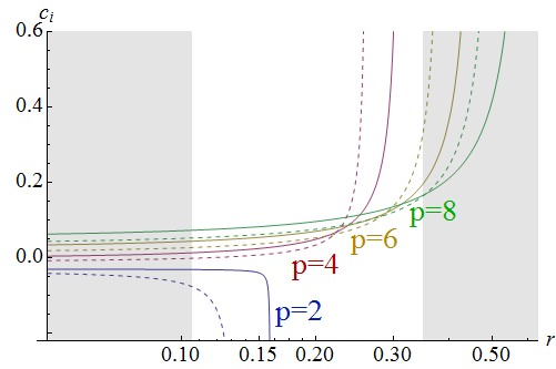
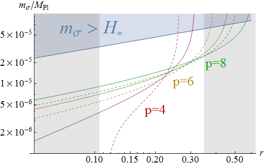
Although the HIM and the intrinsic mass work in the similar ways, only the former squared can be negative and help the chaotic inflation models which predict larger (bluer) tilts than the observation. Therefore, in the right panel of fig. 2, the $p=2$ case does not appear and the $p=4$ and $N=60$ (dashed line) case cannot has a finite $m_{\sigma}$ for $r<0.12$. On the other hand, the $p=2$ lines rapidly drops in the left panel because the additional contribution to the scalar curvature perturbation can work only for $r<r^{(\phi)}$.

It is known well that the $n_{s}$ - $r$ plane is useful to distinguish single slow-roll inflation models. Especially, the prediction of the chaotic inflation model can be expressed as a definite point on the plane if the e-folding number $N_{*}$ is given. Therefore the constraint on the plane is a powerful way to favor or exclude the model. However, if the curvaton is added to the chaotic inflation, since the curvaton mass $m_{\sigma,{\rm eff}}^{2}$ during inflation and its relative contribution to the curvature perturbation $R$ are the additional parameters, the model prediction occupies a finite region on the $n_{s}$-$r$ plane. One can eliminate $R$ from eqs.(14) and (19) and obtains,

This equation describes how the curvaton can change the prediction for {$n_{s},r$} of the original $\phi^{p}$ chaotic inflation models. If the curvaton mass is negligible ($\eta_{\sigma}\to 0$), one finds $\Delta r=-4p\Delta n_{s}$. A finite curvaton mass changes the gradient of the line. For $\eta_{\sigma}<-2\epsilon/p$, the gradient becomes positive. Note since $R$ is positive in our scenario, $\Delta r$ is always negative.

Fig. 3 shows the region where the curvaton models in the chaotic inflation can access on the {$n_{s},r$} plane. Since in the HIM model the curvaton has a negative mass squared the accessible region is larger than the intrinsic mass model. The figure indicates that the models are heavily degenerated especially in the observationally favored region.

Let us stress that the results of this section are applicable to not only curvaton models but also the other type of the curvaton-like models.

First, let us consider the tensor tilt $n_{T}$. Taking the derivative of eq. (9), one finds

Combining the above expression for $n_{T}$ with eq. (10), we obtain so-called “the consistency relation” of single slow-roll inflation models as [31]

On the other hand, once the additional contribution to the curvature perturbations exists, the tensor-to-scalar ratio is modified as shown in the previous section and hence the above consistency relation would be violated as

In other words, through the above expression, $R$ can be observationally determined by the combination of the tilt of the tensor spectrum $n_{T}$ and the tensor-to-scalar ratio $r$ as

On the other hand, the running of the spectral index of the curvature perturbation in the standard single slow-roll inflation is given by⁴⁴ 4 When one computes the derivatives of the slow-roll parameters, $\mathrm{d}\epsilon/\mathrm{d}\ln k=2\epsilon(2\epsilon-\eta)=4\epsilon^{2}/p$ is useful.

and we also obtain the running in the case with the additional contribution from the curvaton fluctuation as ⁵⁵ 5 One can show useful equations, $\frac{\mathrm{d}\ln R}{\mathrm{d}\ln k}=\frac{4}{p}\epsilon+\frac{2m_{\sigma,{\rm eff}}^{2}}{3H^{2}}$ and $-\frac{\mathrm{d}}{\mathrm{d}\ln k}\frac{1}{1+R}=\frac{\mathrm{d}}{\mathrm{d}\ln k}\frac{R}{1+R}=\frac{R^{2}}{(1+R)^{2}}\left[\frac{4}{p}\epsilon+\frac{2m_{\sigma,{\rm eff}}^{2}}{3H^{2}}\right]$.

where $n_{s}^{\prime}(m_{\sigma})$ denotes the model with the intrinsic mass, $m_{\sigma}$, while $n_{s}^{\prime}(c_{i})$ denotes the model with the HIM, $c_{i}H_{*}^{2}$, during inflation. The first, the second and the third term represent the contributions from the inflaton, the curvaton and their mixture, respectively. Notice the second term has the extra term in the former model because in the latter model, $m_{\sigma,{\rm eff}}^{2}/H_{*}^{2}$ is constant and its derivative vanishes.

Fig. 4 shows $n_{s}^{\prime}$ in the case with the Hubble induced mass (left panel) and the intrinsic mass (right panel). The mass of the curvaton, $m_{\sigma,{\rm eff}}^{2}$, would be determined by the observables with fixing the inflation model as shown in Eq. (20), and hence from the expression (27), $n_{s}^{\prime}$ can be also written in terms of the observables ($n_{s},r,H_{*}$) and the inflationary parameter $(p,N)$. As shown in Eq. (27), since terms originated from the mass of the curvaton $\sigma$ always have the positive contributions to $n_{s}^{\prime}$, they somewhat cancel the negative contribution from the inflaton which is proportional to $\epsilon^{2}$. Thus when $n_{s}^{\prime}$ is negative, its magnitude is comparable or smaller than the original prediction of the inflation and it means that the maximum absolute value of the negative $n_{s}^{\prime}$ is given by ${n_{s}^{\prime}}^{(\phi)}$ listed as

As shown in the previous subsection, the ratio $n_{T}/r$ fixes the relative contribution of the curvaton or the other additional degrees of freedom (see eq. (25)). In other words, it implies how the observed $r$ deviates from the original prediction of a inflation model, namely “the consistency relation”. Therefore if observations fix both $r$ and $n_{T}$ with sufficient accuracy, the most favored inflation model at least in the light of the tensor perturbation is determined without an uncertainty from curvaton-like models. However, the curvaton model is not identified because various curvaton models (e.g. the HIM model or the intrinsic mass model) can produce the same amount of $R$.

Then we need another observable to distinguish curvaton models. The running of the spectrum index $n_{s}^{\prime}$ can be useful for the purpose. As we see in fig. 4, $n_{s}^{\prime}$ predicted by models are different and can work as a discriminator. This is because the parameters in curvaton models are fixed to reproduce the observed $n_{s}$. Thus the differences between models appear in the prediction for $n_{s}^{\prime}$.

Let us consider the plane whose x-axis is $n_{s}^{\prime}$ and y-axis is $R=-1-8n_{T}/r$. Using eqs. (14), (19) and (27), the location on the $\{n_{s}^{\prime},R\}$ plane can be described by $n_{s}$ and $r$. In the two curvaton models, the expressions of $n_{s}^{\prime}$ are given by

where $\epsilon=p/(4N+p)$ in the chaotic inflation model.

In fig. 5 and fig. 6, we demonstrate that the two curvaton models in the $\phi^{p}$ chaotic inflation are distinguishable on the new plane. These figures should be compared with fig. 3. The deviations between the original predictions of the inflation models and the fiducial points (we adopt $\{n_{s},r\}=\{0.945,0.15\},\{0.95,0.1\},\{0.96,0.2\}$ and $\{0.965,0.1\}$, see the red points in fig. 3) reflect the differences on the $n_{s}^{\prime}$-$R$ plane. It should be noted that the consistency relation is satisfied on the x-axis of the $n_{s}^{\prime}$-$R$ plane, namely $R=0$.

Regarding observations, in order to discriminate the curvaton models, typically $\mathcal{O}(10^{-4})$ accuracy in the determination of $n_{s}^{\prime}$ is required. Such a great accuracy may be still challenging in the next generation observations [32, 33]. For example, in ref. [33], the authors argue that 1$\sigma$ uncertainty for $n_{s}^{\prime}$ is larger than $10^{-4}$ even from a combination of CMB and 21cm fluctuation future experiments (i.e. CMBpol + Omniscope). Thus a more advanced observation is required to distinguish the curvaton models.

References

- (1) K. Enqvist and M. S. Sloth, “Adiabatic CMB perturbations in pre - big bang string cosmology,” Nucl. Phys. B 626, 395 (2002) [hep-ph/0109214].
- (2) D. H. Lyth and D. Wands, “Generating the curvature perturbation without an inflaton,” Phys. Lett. B 524, 5 (2002) [hep-ph/0110002].
- (3) T. Moroi and T. Takahashi, “Cosmic density perturbations from late decaying scalar condensations,” Phys. Rev. D 66, 063501 (2002) [hep-ph/0206026].
- (4) P. A. R. Ade et al. [BICEP2 Collaboration], “BICEP2 I: Detection Of B-mode Polarization at Degree Angular Scales,” arXiv:1403.3985 [astro-ph.CO].
- (5) C. T. Byrnes, M. Cortês and A. R. Liddle, arXiv:1403.4591 [astro-ph.CO].
- (6) M. S. Sloth, arXiv:1403.8051 [hep-ph].
- (7) A. D. Linde, “Chaotic Inflation,” Phys. Lett. B 129, 177 (1983).
- (8) A. D. Linde, Contemp. Concepts Phys. 5, 1 (1990) [hep-th/0503203].
- (9) M. Kawasaki, M. Yamaguchi and T. Yanagida, Phys. Rev. Lett. 85, 3572 (2000) [hep-ph/0004243].
- (10) M. Kawasaki, M. Yamaguchi and T. Yanagida, Phys. Rev. D 63, 103514 (2001) [hep-ph/0011104].
- (11) R. Kallosh and A. Linde, JCAP 1011, 011 (2010) [arXiv:1008.3375 [hep-th]].
- (12) R. Kallosh, A. Linde and T. Rube, Phys. Rev. D 83, 043507 (2011) [arXiv:1011.5945 [hep-th]].
- (13) G. Dvali, A. Gruzinov and M. Zaldarriaga, Phys. Rev. D 69, 023505 (2004) [astro-ph/0303591]l
- (14) L. Kofman, astro-ph/0303614;
- (15) M. Zaldarriaga, Phys. Rev. D 69, 043508 (2004) [astro-ph/0306006].
- (16) M. Sasaki and E. D. Stewart, Prog. Theor. Phys. 95, 71 (1996) [astro-ph/9507001];
- (17) D. Wands, K. A. Malik, D. H. Lyth and A. R. Liddle, Phys. Rev. D 62, 043527 (2000) [astro-ph/0003278];
- (18) D. H. Lyth, K. A. Malik and M. Sasaki, JCAP 05,(2005) 004. [astro-ph/0411220].
- (19) K. Ichikawa, T. Suyama, T. Takahashi and M. Yamaguchi, Phys. Rev. D 78, 023513 (2008) [arXiv:0802.4138 [astro-ph]].
- (20) K. Enqvist and T. Takahashi, “Mixed Inflaton and Spectator Field Models after Planck,” JCAP 1310, 034 (2013) [arXiv:1306.5958 [astro-ph.CO]].
- (21) P. A. R. Ade et al. [Planck Collaboration], “Planck 2013 results. XXII. Constraints on inflation,” arXiv:1303.5082 [astro-ph.CO].
- (22) P. A. R. Ade et al. [Planck Collaboration], arXiv:1303.5084 [astro-ph.CO].
- (23) T. Kobayashi and T. Takahashi, Phys. Rev. Lett. 110, 231101 (2013) [arXiv:1303.0242 [astro-ph.CO]].
- (24) T. Matsuda, Phys. Lett. B 659, 783 (2008) [arXiv:0712.2103 [hep-ph]].
- (25) T. Kobayashi, F. Takahashi, T. Takahashi and M. Yamaguchi, JCAP 1310, 042 (2013) [arXiv:1303.6255 [astro-ph.CO]].
- (26) E. D. Stewart, Phys. Rev. D 51, 6847 (1995) [hep-ph/9405389].
- (27) M. Dine, L. Randall and S. D. Thomas, Phys. Rev. Lett. 75, 398 (1995) [hep-ph/9503303].
- (28) M. Kawasaki and T. Takesako, Phys. Lett. B 711, 173 (2012) [arXiv:1112.5823 [hep-ph]].
- (29) M. Kawasaki and T. Takesako, Phys. Lett. B 718, 522 (2012) [arXiv:1208.1323 [hep-ph]].
- (30) M. Kawasaki, F. Takahashi and T. Takesako, JCAP 1304, 008 (2013) [arXiv:1211.4921 [hep-ph]].
- (31) A. R. Liddle and D. H. Lyth, Phys. Lett. B 291, 391 (1992) [astro-ph/9208007].
- (32) J. B. Dent, D. A. Easson and H. Tashiro, Phys. Rev. D 86, 023514 (2012) [arXiv:1202.6066 [astro-ph.CO]].
- (33) K. Kohri, Y. Oyama, T. Sekiguchi and T. Takahashi, “Precise Measurements of Primordial Power Spectrum with 21 cm Fluctuations,” JCAP 1310, 065 (2013) [arXiv:1303.1688 [astro-ph.CO]].
- (34) D. H. Lyth, C. Ungarelli and D. Wands, Phys. Rev. D 67, 023503 (2003) [astro-ph/0208055].
- (35) M. Kawasaki, T. Kobayashi and F. Takahashi, Phys. Rev. D 84, 123506 (2011) [arXiv:1107.6011 [astro-ph.CO]].