跳到论文正文
W Papers独立论文阅读器 arXiv:1404.0885 论文正文 计算阅读时间 · 0%
引用这篇论文根据当前论文元数据生成,正式投稿前建议核对。


License: arXiv.org perpetual non-exclusive license
arXiv:1404.0885v2 [cond-mat.str-el] 23 Jun 2014

Quench dynamics of one-dimensional interacting bosons in a disordered potential: Elastic dephasing and critical speeding-up of thermalization

Marco Tavora1 Affiliation: 1 Department of Physics, New York University, 4 Washington Place, New York, NY 10003, USA
2 Institut für Theoretische Physik, Universität zu Köln, D-50937 Cologne, Germany
   Achim Rosch2 Affiliation: 1 Department of Physics, New York University, 4 Washington Place, New York, NY 10003, USA
2 Institut für Theoretische Physik, Universität zu Köln, D-50937 Cologne, Germany
   Aditi Mitra1 Affiliation: 1 Department of Physics, New York University, 4 Washington Place, New York, NY 10003, USA
2 Institut für Theoretische Physik, Universität zu Köln, D-50937 Cologne, Germany
August 24, 2026
Abstract

The dynamics of interacting bosons in one dimension following the sudden switching on of a weak disordered potential is investigated. On time scales before quasiparticles scatter (prethermalized regime), the dephasing from random elastic forward scattering causes all correlations to decay exponentially fast, but the system remains far from thermal equilibrium. For longer times, the combined effect of disorder and interactions gives rise to inelastic scattering and to thermalization. A novel quantum kinetic equation accounting for both disorder and interactions is employed to study the dynamics. Thermalization turns out to be most effective close to the superfluid-Bose glass critical point where nonlinearities become more and more important. The numerically obtained thermalization times are found to agree well with analytic estimates.

pacs
05.70.Ln, 64.70.Tg, 67.85.-d, 71.30.+h

One of the most challenging questions in strongly correlated systems is understanding the combined effect of disorder and interactions. This old problem has recently received some fresh input both in the form of experiments where ultra-cold gases with tunable interactions and tunable disordered potentials have been realized [1, 2, 3], and in the form of theory where phenomena such as many-body localization have been proposed [4, 5, 6]. These studies indicate that the combined effect of disorder and interactions is most dramatic in the nonequilibrium regime. While even for clean interacting systems, quantum dynamics is poorly understood, disorder adds yet another layer of complexity to the problem.

In this paper we study quench dynamics of a one-dimensional (1dd) interacting Bose gas in a disordered potential. The quench involves a sudden switching on of the disordered potential. Past studies of such quenches have primarily focused on the limit of strong disorder and weak interactions where many-body localization may lead to a breakdown of equilibration [7, 8, 9]. We focus on the complementary regime of strong interactions and weak disorder. More precisely, we investigate a regime where disorder is nominally irrelevant by studying the superfluid side of the superfluid-Bose glass quantum critical point.

A quantum quench drives a system out of equilibrium, and the key question is how the system relaxes. We show that the nonequilibrium bosons generated by the quench can relax by means of two different kinds of scattering processes in the presence of disorder. One is a random elastic forward scattering which leads to dephasing. The second is inelastic scattering arising due to the interplay of disorder and interactions which eventually thermalizes the system. We use a novel quantum kinetic equation that accounts for both disorder and interactions to investigate numerically how the system thermalizes. We also present analytic estimates for the thermalization time. We however do not investigate the role of hydrodynamic long time tails which ultimately dominate equilibration at the longest time scales [10].

Upon approaching a classical or quantum critical point, two competing phenomena can occur: ‘critical slowing down’ arises when the relaxation becomes slower and slower due to the dynamics of larger and larger domains. But also the opposite, ‘critical speeding up’, can occur: due to the abundance of critical fluctuations and the importance of nonlinearities thermalization can become more efficient close to criticality. Both effects can even occur simultaneously. For magnetic quantum-critical points in 3dd metals, for example, electron relaxation becomes more efficient close to the transition while the order parameter relaxes more slowly [11]. A dramatic ‘critical speeding up’ has, for example, recently been observed close to the liquid-gas transition of monopoles in spin-ice [12]. Also experimental, numerical and analytic results on the short [13, 14, 15] and long-time dynamics [16] of the superfluid-Mott transition suggest that the dynamics becomes faster upon approaching the transition. In this case, however, the proximity to integrable points makes the theoretical analysis of equilibration more challenging, a complication absent in our study. We find that the enhanced role of backscattering close to the critical point does give rise to a striking enhancement of equilibration upon approaching the critical point.

The equilibrium phase diagram of 1dd interacting bosons in the limit of weak disorder was studied in Refs. 17, 18, where a Berezenskii-Kosterlitz-Thouless (BKT) transition from the superfluid phase to a Bose-glass phase was identified, for strong disorder see, e.g., Refs. [19, 20, 21], and for quasiperiodic lattices see Refs. [22, 23]. We will study quench dynamics in the regime of weak disorder when bosons are delocalized in the ground state. We will, however, show that out of equilibrium even very weak disorder can be quite potent, causing elastic dephasing and inelastic scattering. These effects will be identified by studying the time-evolution of some key correlation functions and the boson distribution function.

Our quench protocol is as follows. First the bosons are prepared in the ground state of a Hamiltonian HiH_{i} characterized by an interaction parameter KK, and sound velocity uu, Hi=u2​π​∫d​x​[K​(π​Π​(x))2+1K​(∂xϕ⁡(x))2]=∑p≠0u​|p|​ap†​apH_{i}=\frac{u}{2\pi}\int dx\left[K\left(\pi\Pi(x)\right)^{2}+\frac{1}{K}\left(\partial_{x}\phi(x)\right)^{2}\right]=\sum_{p\neq 0}u|p|a_{p}^{\dagger}a_{p}. Π=∂xθ/π\Pi=\partial_{x}\theta/\pi is canonically conjugate to the field ϕ\phi, −∂xϕ/π-\partial_{x}\phi/\pi is the smooth part of the boson density, and the theory is diagonal in terms of ap†,apa_{p}^{\dagger},a_{p}, the creation and annihilation operators for the sound modes [24, 25]. At t=0t=0, a disordered potential is suddenly switched on so that the time evolution from t>0t>0 is governed by the final Hamiltonian Hf=Hi+VdisH_{f}=H_{i}+V_{\rm dis} where,

Vdis=∫dx[−1πη(x)∂xϕ+(ξ∗e2​i​ϕ+ξe−2​i​ϕ)]\displaystyle V_{\rm dis}=\int dx\left[-\frac{1}{\pi}\eta(x)\partial_{x}\phi+\left(\xi^{*}e^{2i\phi}+\xi e^{-2i\phi}\right)\right] (1)

η\eta and ξ\xi are the strength of the forward and backward scattering disorder respectively [24], these are assumed to be time-independent and Gaussian distributed so that disorder-averaging (represented by …¯\overline{\ldots}) gives, η⁡(x)​η​(x′)¯=Df​δ​(x−x′),ξ⁡(x)​ξ∗​(x′)¯=Db​δ​(x−x′)\overline{\eta(x)\eta(x^{\prime})}=D_{f}\delta(x-x^{\prime}),\overline{\xi(x)\xi^{*}(x^{\prime})}=D_{b}\delta(x-x^{\prime}). We find it convenient to define 𝒟b=2​π​Db​uΛ3{\cal D}_{b}=\frac{2\pi D_{b}u}{\Lambda^{3}} and 𝒟f=Df​αu2{\cal D}_{f}=D_{f}\frac{\alpha}{u^{2}} as dimensionless strength of the forward and backward scattering disorder, respectively where Λ=u/α\Lambda=u/\alpha is a UV cutoff. Note that K→∞K\rightarrow\infty is the limit of non-interacting bosons, while K=1K=1 corresponds to hard-core bosons (free fermions), with the superfluid-Bose glass critical point located near K=3/2K=3/2 [24].

We will study the time evolution after the quench of the boson density-density correlation function Rϕ​ϕR_{\phi\phi}, and the single-particle correlation function Rθ​θR_{\theta\theta}, the latter being a measure of the superfluidity in the system. These quantities in the language of bosonization are,

Rϕ​ϕ​(r,t)=⟨ψi|ei​Hf​t​e2​i​ϕ​(r)​e−2​i​ϕ​(0)​e−i​Hf​t|ψi⟩\displaystyle R_{\phi\phi}(r,t)=\langle\psi_{i}|e^{iH_{f}t}e^{2i\phi(r)}e^{-2i\phi(0)}e^{-iH_{f}t}|\psi_{i}\rangle (2)
Rθ​θ​(r,t)=⟨ψi|ei​Hf​t​ei​θ​(r)​e−i​θ​(0)​e−i​Hf​t|ψi⟩\displaystyle R_{\theta\theta}(r,t)=\langle\psi_{i}|e^{iH_{f}t}e^{i\theta(r)}e^{-i\theta(0)}e^{-iH_{f}t}|\psi_{i}\rangle (3)

where |ψi⟩|\psi_{i}\rangle is the state before the quench (the ground-state of HiH_{i}). Note that Rϕ​ϕR_{\phi\phi} is the correlator for the component of the density that oscillates at 2​π​ρ02\pi\rho_{0} (where ρ0\rho_{0} is the average boson density). We choose to study this because in the vicinity of the superfluid-Bose glass critical point, charge density wave fluctuations dominate.

We employ a Keldysh path-integral formalism wherein the expectation value of the observable Ra​aR_{aa} (where a=θ/ϕa=\theta/\phi) is given by

⟨ψi|Ra​a​(t)|ψi⟩=T​r​[e−i​Hf​t​|ψi⟩​⟨ψi|​ei​Hf​t​Ra​a]\displaystyle\langle\psi_{i}|R_{aa}(t)|\psi_{i}\rangle=Tr\left[e^{-iH_{f}t}|\psi_{i}\rangle\langle\psi_{i}|e^{iH_{f}t}R_{aa}\right]
=∫𝒟⁡[ϕc​l,ϕq]​ei⁡(S0+Sdis)​Ra​a​[ϕc​l/q​(t),θc​l/q​(t)]\displaystyle=\int{\cal D}\left[\phi_{cl},\phi_{q}\right]e^{i\left(S_{0}+S_{\rm dis}\right)}R_{aa}\left[\phi_{cl/q}(t),\theta_{cl/q}(t)\right] (4)

where ϕc​l,q,θc​l,q\phi_{cl,q},\theta_{cl,q} are linear combinations of the fields ϕ±,θ±\phi_{\pm},\theta_{\pm} in the two-time Keldysh formalism [26]. Above, S0S_{0} captures the correlators of the clean interacting Bose gas after the quench, exactly known within our Luttinger liquid approximation [27]. SdisS_{\rm dis} contains the forward and backward scattering disorder. While the forward scattering disorder may be treated exactly, we will treat the backward scattering disorder perturbatively. Within the Keldysh formalism, disorder-averaging may be carried out without the complication of introducing replicas

⟨ψi|Ra​a​(t)|ψi⟩¯=\displaystyle\overline{\langle\psi_{i}|R_{aa}(t)|\psi_{i}\rangle}= ∫𝒟⁡[η,ξ,ξ∗]​e−η2​(x)2​Df​e−ξ⁡(x)​ξ∗​(x)Db\displaystyle\int{\cal D}\left[\eta,\xi,\xi^{*}\right]e^{-\frac{\eta^{2}(x)}{2D_{f}}}e^{-\frac{\xi(x)\xi^{*}(x)}{D_{b}}} (5)
×⟨ψi|Ra​a​(t)|ψi⟩\displaystyle\times\langle\psi_{i}|R_{aa}(t)|\psi_{i}\rangle

Writing Ra​a=Ra​a(0)+Ra​a(1)+…R_{aa}=R^{(0)}_{aa}+R^{(1)}_{aa}+\ldots where R(i)R^{(i)} is 𝒪⁡(Dbi){\cal O}\left(D_{b}^{i}\right), to leading order, only the forward scattering disorder affects the correlators, but already at this order elastic dephasing effects will be apparent. To see this note that when Db=0D_{b}=0, HfH_{f} may be diagonalized Hf​(Db=0)=∑pu​|p|​Γp†​ΓpH_{f}(D_{b}=0)=\sum_{p}u|p|\Gamma_{p}^{\dagger}\Gamma_{p} where Γp=ap+η~pu​|p|\Gamma_{p}=a_{p}+\frac{\tilde{\eta}_{p}}{u|p|}, and η~p=KLL​|p|2​πe−α|p|/2∫dxη(x)e−i​p​x\tilde{\eta}_{p}=\frac{\sqrt{K}}{L}\sqrt{\frac{L|p|}{2\pi}}e^{-\alpha|p|/2}\int dx\eta(x)e^{-ipx}, LL being the system size. The quench creates a highly nonequilibrium distribution of the Γp\Gamma_{p} quasiparticles so that, before disorder averaging, the leading order correlators at a time tt after the disorder quench are [28],

Rϕ​ϕ(0)​(r,t)=⟨ψi|e2​i​ϕ​(r,t)​e−i​2​ϕ​(0,t)|ψi⟩Df=0\displaystyle R^{(0)}_{\phi\phi}(r,t)=\langle\psi_{i}|e^{2i\phi(r,t)}e^{-i2\phi(0,t)}|\psi_{i}\rangle_{D_{f}=0}
×e−i​Ku∑ϵ=±[∫rr+ϵ​u​tdyη(y)−∫0ϵ​u​tdyη(y)]\displaystyle\times e^{-\frac{iK}{u}\sum_{\epsilon=\pm}\left[\int_{r}^{r+\epsilon ut}dy\eta(y)-\int_{0}^{\epsilon ut}dy\eta(y)\right]} (6)
Rθ​θ(0)​(r,t)=⟨ψi|ei​θ​(r,t)​e−i​θ​(0,t)|ψi⟩Df=0\displaystyle R^{(0)}_{\theta\theta}(r,t)=\langle\psi_{i}|e^{i\theta(r,t)}e^{-i\theta(0,t)}|\psi_{i}\rangle_{D_{f}=0}
×e−i2​u​[∫r−u​tr+u​td​y​η​(y)−∫−u​tu​td​y​η​(y)]\displaystyle\times e^{-\frac{i}{2u}\left[\int_{r-ut}^{r+ut}dy\eta(y)-\int_{-ut}^{ut}dy\eta(y)\right]} (7)

The correlators are what they would have been in the absence of the forward scattering disorder (Df=0D_{f}=0), but multiplied by random phases. These phases arise because the quench creates excited left and right moving quasiparticles which as they travel along the chain pick up random phases due to the forward scattering disorder. Thus the operator at position rr will be affected by phases picked up in the region [r−u​t,r]\left[r-ut,r\right] by the right movers, and phases picked up in the region [r+u​t,r]\left[r+ut,r\right] by the left movers.

Due to these random phases, disorder averaging leads to dephasing that causes the correlators to decay exponentially in time or position,

R¯ϕ​ϕ(0)(r,t)=[11+r2​Λ2]2​Kexp{−K2​Dfu[\displaystyle\overline{R}^{(0)}_{\phi\phi}\left(r,t\right)=\left[\frac{1}{\sqrt{1+r^{2}\Lambda^{2}}}\right]^{2K}\exp\biggl\{-\frac{K^{2}D_{f}}{u}\biggl[
2​t​Θ​(|r|/u−2​t)+(4​t−|r|/u)​Θ​(2​t−|r|/u)​Θ​(|r|/u−t)\displaystyle 2t\Theta(|r|/u-2t)+\left(4t-|r|/u\right)\Theta(2t-|r|/u)\Theta(|r|/u-t)
+3|r|Θ(t−|r|/u)]}\displaystyle+3|r|\Theta(t-|r|/u)\biggr]\biggr\}
R¯θ​θ(0)(r,t)=[11+r2​Λ2]1/(2​K)exp{−Df4​u[2t\displaystyle\overline{R}^{(0)}_{\theta\theta}\left(r,t\right)=\left[\frac{1}{\sqrt{1+r^{2}\Lambda^{2}}}\right]^{1/(2K)}\exp\biggl\{-\frac{D_{f}}{4u}\biggl[2t
−(2t−|r|/u)Θ(2t−|r|/u)]}\displaystyle-(2t-|r|/u)\Theta(2t-|r|/u)\biggr]\biggr\} (8)

Above Θ\Theta is the Heaviside function. Thus the disorder-averaged correlators are found to decay exponentially with time for short times u​t<r/2ut<r/2, with a crossover to a steady-state behavior with an exponential decay in position at long times (u​t>r/2ut>r/2 for Rθ​θR_{\theta\theta} and u​t>rut>r for Rϕ​ϕR_{\phi\phi}). It is interesting to contrast this behavior with the situation in equilibrium. There the forward-scattering disorder also imposes an exponential decay in position of the density correlator Rϕ​ϕeq∼1r2​K​e−2​K2​Df​|r|u2R^{\rm eq}_{\phi\phi}\sim\frac{1}{r^{2K}}e^{-\frac{2K^{2}D_{f}|r|}{u^{2}}}, but does not affect the single-particle propagator at all Rθ​θeq∼1/r1/(2​K)R_{\theta\theta}^{\rm eq}\sim 1/r^{1/(2K)}, implying that it cannot suppress superfluidity. Only backward scattering disorder suppresses superfluidity in equilibrium, eventually causing a transition to the Bose-glass phase [17]. In contrast, our leading order result shows that when the system is quenched, even forward scattering strongly affects superfluidity due to random dephasing caused by the emitted nonequilibrium quasiparticles.

Thus even though the disorder is weak, and even though we are in the short time or intermediate time regime where the full effect of the disorder has not yet set in, disorder is very effective in destroying the superfluidity due to random dephasing. Moreover, in stark contrast to equilibrium, it is the forward scattering disorder which is the most potent in this prethermalized regime as random dephasing caused by it also makes the backward scattering disorder more “irrelevant” than in equilibrium. Thus while superfluidity is destroyed, the phase that replaces it is not a backward scattering disorder induced localized phase either. In fact, as we discuss in detail below, the role of backward scattering disorder is to facilitate inelastic scattering, causing the system to thermalize into a delocalized high temperature phase.

We now discuss the long time regime where inelastic effects are important. Even in clean interacting systems, inelastic effects after a quench set in, however for the Luttinger model, where only forward scattering interactions are retained, the clean system is incapable of thermalizing. In contrast once disorder is present, then the combined effect of disorder and interactions can cause inelastic scattering leading to thermalization. We will now explore this phenomena. Of course for free fermions with disorder (K=1K=1), there is again no inelastic scattering, however our treatment is valid for strong attractive (albeit forward scattering) interactions and weak disorder.

Refer to caption
Figure 1: Main panel: Time evolution of q​n​(q)qn(q) for a quench where K=3K=3 and the quench amplitude Teff,0=0.024T_{\rm eff,0}=0.024. The system thermalizes with n⁡(q)n(q) approaching neq​(q)=1eu​|q|/Teq−1n_{\rm eq}(q)=\frac{1}{e^{u|q|/T_{\rm eq}}-1} with TeqT_{\rm eq} determined from energy conservation. Inset: Time-evolution of u​[q​n​(q)]q=0=Teffu\left[qn(q)\right]_{q=0}=T_{\rm eff} for K=3K=3 and 3/23/2. Teff​(t=0)=Teff,0T_{\rm eff}(t=0)=T_{\rm eff,0} and approaches TeqT_{\rm eq} at long times. u=1u=1, q,tq,t are in units of Λ,[8​𝒟b​Λ/π]−1\Lambda,\left[8{\cal D}_{b}\Lambda/\pi\right]^{-1} respectively.

The quantum quench generates nonequilibrium quasiparticles with density np​(t)=⟨ψi​(t)|Γp†​Γp|ψi​(t)⟩n_{p}(t)=\langle\psi_{i}(t)|\Gamma_{p}^{\dagger}\Gamma_{p}|\psi_{i}(t)\rangle. At short times γ0​t<1\gamma_{0}t<1 (below we give an estimate for γ0\gamma_{0}), these may be considered to be almost free, this is the so called prethermalized regime [29, 30, 31, 32, 33] discussed above. In contrast, at longer times, these quasiparticles eventually scatter among each other, with the distribution function evolving according to the quantum kinetic equation [28]

u​|p|Λ2​∂∂t​np​(t)\displaystyle\frac{u|p|}{\Lambda^{2}}\frac{\partial}{\partial t}{n}_{p}(t) =−i​π​K2{np(t)[ΣR−ΣA](p,t)\displaystyle=-\frac{i\pi K}{2}\biggl\{{n}_{p}(t)\left[\Sigma^{R}-\Sigma^{A}\right](p,t) (9)
−12[ΣK(p,t)−(ΣR−ΣA)(p,t)]}\displaystyle-\frac{1}{2}\left[\Sigma^{K}(p,t)-(\Sigma^{R}-\Sigma^{A})(p,t)\right]\biggr\}

ΣR,A,K\Sigma^{R,A,K} are the self-energies to 𝒪⁡(𝒟b){\cal O}({\cal D}_{b}), and themselves depend on the nonequilibrium population np​(t)n_{p}(t). A kinetic equation similar to the one above was derived for a commensurate periodic potential [16]. For the disordered problem, the derivation follows analogously. Due to the interaction vertex being of the form e2​i​ϕe^{2i\phi}, a key feature of the kinetic equation is that it allows for multi-particle scattering between bosons. Besides this, it has all the usual properties of a kinetic equation in that it conserves energy, and the right hand side vanishes when npn_{p} is the Bose distribution function. We solve the kinetic equation numerically, where the initial condition entering the kinetic equation is the nonequilibrium quasiparticle density npn_{p} generated by the quench. Note that the kinetic equation has been obtained after a leading order gradient expansion and in doing so has lost some of the initial memory effects, and is therefore not valid at very short times after the quench. We smoothly connect between the short time dynamics and the long time dynamics of the kinetic equation by perturbatively evolving np​(t)n_{p}(t) forward in time at short times, and use this distribution as the initial condition for the kinetic equation. For u​|p|≪Λu|p|\ll\Lambda, such a perturbative short time evolution gives [28]

np​(t≃0)=⟨ψi|Γp†​Γp|ψi⟩=Tefff+Teffbu​|p|=Teff,0u​|p|\displaystyle n_{p}(t\simeq 0)=\langle\psi_{i}|\Gamma_{p}^{\dagger}\Gamma_{p}|\psi_{i}\rangle=\frac{T_{\rm eff}^{f}+T_{\rm eff}^{b}}{u|p|}=\frac{T_{\rm eff,0}}{u|p|} (10)

where Teff,0=Tefff+TeffbT_{\rm eff,0}=T_{\rm eff}^{f}+T_{\rm eff}^{b} with Tefff=K​𝒟f​Λ2​π,Teffb=Λ​8​π​K​𝒟b​[Γ⁡(2​K−2)Γ⁡(2​K)]T_{\rm eff}^{f}=\frac{K{\cal D}_{f}\Lambda}{2\pi},T_{\rm eff}^{b}=\Lambda 8\pi K{\cal D}_{b}\left[\frac{\Gamma(2K-2)}{\Gamma(2K)}\right]. Thus the density is a sum of two terms, one proportional to the strength of the forward scattering disorder and the second proportional to the strength of the backward scattering disorder. The symbol np​(t≃0)n_{p}(t\simeq 0) is used to imply that this distribution is obtained after an initial time-evolution. At long wavelengths, the distribution np​(t≃0)n_{p}(t\simeq 0) has the appearance of an effective temperature, however unlike a true temperature where for u​|p|≥Teff,0u|p|\geq T_{\rm eff,0}, the distribution function is exponentially suppressed, for our case, the distribution function maintains a slow power-law decay with momentum upto energy scales of the order of the cutoff Λ\Lambda. We will use Teff,0T_{\rm eff,0} as a measure of the quench amplitude and all energy scales will be measured in units of Λ\Lambda.

We now present results for the numerical solution of the kinetic equation for a point far away (K=3K=3) and at (K=3/2K=3/2) the superfluid-Bose glass critical point. In the main panel of Fig. 1 q​n​(q)qn(q) is plotted at different times after the quench, and is found to reach thermal equilibrium q​neq=qeu​|q|/Teq−1qn_{\rm eq}=\frac{q}{e^{u|q|/T_{\rm eq}}-1}, TeqT_{\rm eq} being determined from energy conservation. The high-qq modes thermalize the fastest, thus the thermalization time is set by the behavior of the long-wavelength modes, an observation which will allow us to make analytic estimates for the thermalization time. The numerics also show that the relaxation to equilibrium is not determined by a single time-scale [34] and therefore not described by a single exponential function. This is most directly seen by studying how u​[q​n​(q)]q=0=Teffu\left[qn(q)\right]_{q=0}=T_{\rm eff} approaches TeqT_{\rm eq} starting from its initial value of Teff,0T_{\rm eff,0} (see insets of Figs 1 and 2). Inset of Fig. 1 shows that the system thermalizes much faster at the critical point K=3/2K=3/2 in comparison to away from it (see also [28]). The inset of Fig. 2 clearly shows at least two different relaxation rates appear in the dynamics. Below we discuss these rates analytically.

Since the longest wavelength mode relaxes the slowest, let us consider the out-scattering rate in the long wavelength limit,

γ⁡(p,t)=(π​K2)​i⁡(ΣR−ΣA)u​|p|→p→0\displaystyle\!\!\gamma(p,t)=\!\!\left(\frac{\pi K}{2}\right)\frac{i(\Sigma^{R}-\Sigma^{A})}{u|p|}\xrightarrow{p\rightarrow 0}
=4​K​𝒟b​∫−∞∞d⁡(Λ​τ)​sin⁡[2​K​tan−1⁡Λ​τ]​(Λ​τ)​e−I⁡(t,τ)\displaystyle=4K{\cal D}_{b}\!\!\int_{-\infty}^{\infty}\!\!\!d(\Lambda\tau)\sin\left[2K\tan^{-1}{\Lambda\tau}\right]\left(\Lambda\tau\right)e^{-I(t,\tau)} (11)

where I⁡(t,τ)=2​K​∫0∞d​qq​e−α​q​[1+2​nq​(t)]​[1−cos⁡(q​u​τ)]{I}(t,\tau)\!\!=2K{\int\limits_{0}^{\infty}{{{dq}\over q}}}{e^{-\alpha q}}\left[1+2n_{q}(t)\right]\left[{1-\cos\left(qu\tau\right)}\right]. Two time-scales may be extracted from Eq. (11). One is γ0−1\gamma_{0}^{-1}, the time-scale for leaving the prethermalized regime, and the second is γth−1\gamma_{\rm th}^{-1}, the thermalization time when the system is weakly perturbed from thermal equilibrium. To determine the former, we substitute np​(t≃0)n_{p}(t\simeq 0) into Eq. (11) to obtain, γ0∼𝒟b​Teff,0∼𝒟b​(𝒟f+b​𝒟b)\gamma_{0}\sim{\cal D}_{b}T_{\rm eff,0}\sim{\cal D}_{b}\left({\cal D}_{f}+b{\cal D}_{b}\right).

As the system evolves, the distribution function approaches thermal equilibrium. The time-scale γth−1\gamma_{\rm th}^{-1} for the final approach to thermal equilibrium may be estimated by substituting np=1eu​|p|/Teq−1n_{p}=\frac{1}{e^{u|p|/T_{\rm eq}}-1} in Eq. (11). This yields a thermalization rate of γth∼𝒟b​(Teq)2​K−2\gamma_{\rm th}\sim{\cal D}_{b}\left(T_{\rm eq}\right)^{2K-2}. Since, Teq∼Teff,0T_{\rm eq}\sim\sqrt{T_{\rm eff,0}} for small quench amplitudes [28],

γth∼𝒟b​[Teff,0]K−1\displaystyle\gamma_{\rm th}\sim{\cal D}_{b}\left[T_{\rm eff,0}\right]^{K-1} (12)

Our numerical results show that high-energy modes relax sufficiently fast such that the total time needed for thermalization can be estimated from tth∼γth−1t_{\rm th}\sim\gamma_{\rm th}^{-1}. The relaxation rate towards thermal equilibrium obtained from the long time tail of the time-evolution is shown in the main panel of Fig. 2, and agrees well with γth\gamma_{\rm th}. Note that the dramatic reduction of thermalization time on approaching the superfluid Bose-glass critical point is due to the backward scattering disorder becoming more relevant, facilitating thermalization. We emphasize that our results are valid as long as the backscattering disorder is a weak perturbation, which is the case for K>3/2K>3/2 where 𝒟b{\cal D}_{b} is RG irrelevant. While our expressions remain well defined for 1<K<3/21<K<3/2, they clearly break-down in the hard core boson (or free fermion limit), where the perturbative expression for the density (see TeffbT_{\rm eff}^{b}), and the zero temperature out-scattering rate γth∼𝒟b​∫1∞d​τ​1/τ2​K−1\gamma_{\rm th}\sim{\cal D}_{b}\int_{1}^{\infty}d\tau 1/\tau^{2K-1} acquire infrared divergences [28].

To summarize, we have studied quench dynamics in a system where both interactions and disorder are present. A key effect of the disorder is to give rise to random forward scattering induced elastic dephasing, important even at short times which destroys superfluidity. At longer times, the interplay of disorder and interactions leads to thermalization which is strongly enhanced close to the superfluid-Bose glass transition. Both in the short-time elastic dephasing regime, and the long-time thermal regime, correlations decay exponentially, however one may differentiate between these two regimes by an echo [35] experiment: an echo visible in the short-time dephasing regime will be suppressed exponentially when inelastic scattering dominates. The two regimes may also be identified by the length scale determining the decay of the correlations which is DfD_{f} in the elastic dephasing regime, and TeqT_{\rm eq} in the thermal regime. The dephasing dominated regime should also be observable in short-time numerical simulations on disordered lattice systems. An interesting direction is to study quenches on the insulating side of the superfluid-Bose glass transition where the growth of disorder under renormalization competes with dephasing and decoherence arising from the nonequilibrium population of quasiparticles.

Refer to caption
Figure 2: The thermalization rate γ\gamma obtained from the long time tail agrees well with the analytic estimate which for small quench amplitudes is γth∼𝒟b​(Teff,0)K−1\gamma_{\rm th}\sim{\cal D}_{b}\left(T_{\rm eff,0}\right)^{K-1}. Inset: The relaxation rates for K=3K=3 and 3/23/2 (the latter has been scaled down). For K=3K=3, at short (Teff≃Teff,0T_{\rm eff}\simeq T_{\rm eff,0}) and long times (Teff≃TeqT_{\rm eff}\simeq T_{\rm eq}) the relaxation rates agree well with γ0\gamma_{0}, γth\gamma_{\rm th} respectively indicated by the dashed lines. For K=3/2K=3/2, the relaxation rate at long times agrees well with γth\gamma_{\rm th}.

Acknowledgements: This work was supported by NSF-DMR 1303177 (AM,MT), the Simons Foundation (AM), and the SFB TR12 of the DFG (AR).

References

Supplementary Material for ”Quench dynamics of one-dimensional interacting bosons in a disordered potential”

The supplementary material covers:
1. Evaluation of the correlators after the quench when there is no backward scattering (Db=0D_{b}=0) but only forward scattering.
2. Derivation of the quantum kinetic equation in the presence of disorder and interactions.
3. Estimation of equilibrium temperature from energy conservation.
4. Perturbative time evolution of the density at short times.

I Correlation functions after the quench in the presence of a forward scattering disorder potential (Db=0D_{b}=0)

It is convenient to define boson creation and annihilation operators ap,ap†a_{p},a_{p}^{\dagger}, such that

ϕ⁡(x)=−(NR+NL)​π​xL\displaystyle\phi(x)=-(N_{R}+N_{L})\frac{\pi x}{L}
−i​π​KL∑p≠0(L​|p|2​π)1/21pe−α|p|/2−ipx(ap†+a−p),\displaystyle-\frac{i\pi\sqrt{K}}{L}\sum_{p\neq 0}\left(\frac{L|p|}{2\pi}\right)^{1/2}\frac{1}{p}e^{-\alpha|p|/2-ipx}\left(a_{p}^{\dagger}+a_{-p}\right), (S13)
θ⁡(x)=(NR−NL)​π​xL\displaystyle\theta(x)=(N_{R}-N_{L})\frac{\pi x}{L}
+i​πL​K∑p≠0(L​|p|2​π)1/21|p|e−α|p|/2−ipx(ap†−a−p).\displaystyle+\frac{i\pi}{L\sqrt{K}}\sum_{p\neq 0}\left(\frac{L|p|}{2\pi}\right)^{1/2}\frac{1}{|p|}e^{-\alpha|p|/2-ipx}\left(a_{p}^{\dagger}-a_{-p}\right). (S14)

Λ=u​α−1\Lambda=u\alpha^{-1} is an ultra-violet cutoff, and LL is the system size. The initial Hamiltonian before the quench can now be written as

Hi=∑p≠0u​|p|​ap†​ap\displaystyle H_{i}=\sum_{p\neq 0}u|p|a_{p}^{\dagger}a_{p} (S15)

When after a quench, only a forward scattering disorder is present, the final Hamiltonian may also be diagonalized exactly

Hf​(Db=0)=∑pu​|p|​Γp†​Γp\displaystyle H_{f}(D_{b}=0)=\sum_{p}u|p|\Gamma_{p}^{\dagger}\Gamma_{p} (S16)

where

Γp\displaystyle\Gamma_{p} =\displaystyle= ap+η~pu​|p|\displaystyle a_{p}+\frac{\tilde{\eta}_{p}}{u|p|} (S17)
η~p\displaystyle\tilde{\eta}_{p} =\displaystyle= KLL​|p|2​πe−α|p|/2∫dxη(x)e−i​p​x\displaystyle\frac{\sqrt{K}}{L}\sqrt{\frac{L|p|}{2\pi}}e^{-\alpha|p|/2}\int dx\eta(x)e^{-ipx} (S18)

Note that the new Γp,Γp†\Gamma_{p},\Gamma_{p}^{\dagger} fields correspond to defining a new field ϕ~\tilde{\phi} that is related to the ϕ\phi field by a simple shift,

ϕ~​(x)=ϕ⁡(x)−Ku​∫xd​y​η​(y)\displaystyle\tilde{\phi}(x)=\phi(x)-\frac{K}{u}\int^{x}dy\eta(y) (S19)

where

ϕ~​(x)=−(NR+NL)​π​xL\displaystyle\tilde{\phi}(x)=-(N_{R}+N_{L})\frac{\pi x}{L}
−i​π​KL∑p≠0(L​|p|2​π)1/21pe−α|p|/2−ipx(Γp†+Γ−p)\displaystyle-\frac{i\pi\sqrt{K}}{L}\sum_{p\neq 0}\left(\frac{L|p|}{2\pi}\right)^{1/2}\frac{1}{p}e^{-\alpha|p|/2-ipx}\left(\Gamma_{p}^{\dagger}+\Gamma_{-p}\right) (S20)

Since Γp​(t)=Γp​(0)​e−i​u​|p|​t=(ap​(0)+η~pu​|p|)​e−i​u​|p|​t\Gamma_{p}(t)=\Gamma_{p}(0)e^{-iu|p|t}=\left(a_{p}(0)+\frac{\tilde{\eta}_{p}}{u|p|}\right)e^{-iu|p|t},

ϕ(x,t)=−i​π​KL∑p≠0L​|p|2​π1pe−α|p|/2e−i​p​x\displaystyle\phi(x,t)\!\!=-\frac{i\pi\sqrt{K}}{L}\sum_{p\neq 0}\sqrt{\frac{L|p|}{2\pi}}\frac{1}{p}e^{-\alpha|p|/2}e^{-ipx}
[{ap†(t)+a−p(t)}Df=0\displaystyle\left[\{a_{p}^{\dagger}(t)+a_{-p}(t)\}_{D_{f}=0}\right.
+η~p∗u​|p|(ei​u​|p|​t−1)+η~−pu​|p|(e−i​u​|p|​t−1)]\displaystyle\left.+\frac{\tilde{\eta}_{p}^{*}}{u|p|}\left(e^{iu|p|t}-1\right)+\frac{\tilde{\eta}_{-p}}{u|p|}\left(e^{-iu|p|t}-1\right)\right] (S21)
=ϕ​(x,t)Df=0−K2​π​u​∫−∞∞d​y​η​(y)\displaystyle=\phi(x,t)_{D_{f}=0}-\frac{K}{2\pi u}\int_{-\infty}^{\infty}dy\eta(y)
×[tan−1(x−y+u​tα)+tan−1(x−y−u​tα)\displaystyle\times\left[\tan^{-1}\left(\frac{x-y+ut}{\alpha}\right)+\tan^{-1}\left(\frac{x-y-ut}{\alpha}\right)\right.
−2tan−1(x−yα)]\displaystyle\left.-2\tan^{-1}\left(\frac{x-y}{\alpha}\right)\right] (S22)

Above we have not written the zero mode explicitly. Taking α=0\alpha=0 so that tan−1⁡(x)=π2​[θ⁡(x)−θ⁡(−x)]\tan^{-1}(x)=\frac{\pi}{2}\left[\theta(x)-\theta(-x)\right],

ϕ⁡(x,t)=ϕ​(x,t)Df=0−K2​u​[∫xx+u​td​y​η​(y)+∫xx−u​td​y​η​(y)]\displaystyle\phi(x,t)=\phi(x,t)_{D_{f}=0}-\frac{K}{2u}\left[\int_{x}^{x+ut}dy\eta(y)+\int_{x}^{x-ut}dy\eta(y)\right]
(S23)

Similarly for θ\theta we find

θ(x,t)=i​πL​K∑p≠0L​|p|2​π1|p|e−α|p|/2e−i​p​x\displaystyle\theta(x,t)\!\!=\frac{i\pi}{L\sqrt{K}}\sum_{p\neq 0}\sqrt{\frac{L|p|}{2\pi}}\frac{1}{|p|}e^{-\alpha|p|/2}e^{-ipx}
[{ap†(t)−a−p(t)}Df=0\displaystyle\left[\{a_{p}^{\dagger}(t)-a_{-p}(t)\}_{D_{f}=0}\right.
+η~p∗u​|p|(ei​u​|p|​t−1)−η~−pu​|p|(e−i​u​|p|​t−1)]\displaystyle\left.+\frac{\tilde{\eta}_{p}^{*}}{u|p|}\left(e^{iu|p|t}-1\right)-\frac{\tilde{\eta}_{-p}}{u|p|}\left(e^{-iu|p|t}-1\right)\right] (S24)

The above implies

θ⁡(x,t)=θ​(x,t)Df=0−12​π​u​∫−∞∞d​y​η​(y)\displaystyle\theta(x,t)=\theta(x,t)_{D_{f}=0}-\frac{1}{2\pi u}\int_{-\infty}^{\infty}dy\eta(y)
×[tan−1⁡(u​t+x−yα)+tan−1⁡(u​t−x+yα)]\displaystyle\times\left[\tan^{-1}\left(\frac{ut+x-y}{\alpha}\right)+\tan^{-1}\left(\frac{ut-x+y}{\alpha}\right)\right] (S25)
=θ​(x,t)Df=0−12​u​∫x−u​tx+u​td​y​η​(y)\displaystyle=\theta(x,t)_{D_{f}=0}-\frac{1}{2u}\int_{x-ut}^{x+ut}dy\eta(y) (S26)

Thus the time-evolution of the fields after the quench is the same as that for the clean system (ϕ​(x,t)Df=0,θ​(x,t)Df=0\phi(x,t)_{D_{f}=0},\theta(x,t)_{D_{f}=0}) but with additive corrections coming from random forward scattering.

Let us now evaluate the disorder averaged density correlator,

⟨e2​i​ϕ​(x,t)​e−2​i​ϕ​(0,t)⟩¯=⟨e2​i​ϕ​(x,t)​e−2​i​ϕ​(0,t)⟩Df=0\displaystyle\overline{\langle e^{2i\phi(x,t)}e^{-2i\phi(0,t)}\rangle}=\langle e^{2i\phi(x,t)}e^{-2i\phi(0,t)}\rangle_{D_{f}=0}
×e−i​Ku​[∫xx+u​td​y​η​(y)+∫xx−u​td​y​η​(y)−∫0u​td​y​η​(y)−∫0−u​td​y​η​(y)]¯\displaystyle\times\overline{e^{-\frac{iK}{u}\left[\int_{x}^{x+ut}dy\eta(y)+\int_{x}^{x-ut}dy\eta(y)-\int_{0}^{ut}dy\eta(y)-\int_{0}^{-ut}dy\eta(y)\right]}} (S27)

Defining η⁡(x)=1L​∑kηk​ei​k​x\eta(x)=\frac{1}{\sqrt{L}}\sum_{k}\eta_{k}e^{ikx},

e−i​Ku​[∫xx+u​td​y​η​(y)+∫xx−u​td​y​η​(y)−∫0u​td​y​η​(y)−∫0−u​td​y​η​(y)]¯\displaystyle\overline{e^{-\frac{iK}{u}\left[\int_{x}^{x+ut}dy\eta(y)+\int_{x}^{x-ut}dy\eta(y)-\int_{0}^{ut}dy\eta(y)-\int_{0}^{-ut}dy\eta(y)\right]}}
=ei​Ku​L​∑k2​ηki​k​(1−cos⁡(k​u​t))​(ei​k​x−1)¯\displaystyle=\overline{e^{\frac{iK}{u\sqrt{L}}\sum_{k}\frac{2\eta_{k}}{ik}(1-\cos(kut))(e^{ikx}-1)}}
=e2​i​Ku​L​∑k>0(ηk​fk+ηk∗​fk∗)¯\displaystyle=\overline{e^{\frac{2iK}{u\sqrt{L}}\sum_{k>0}\left(\eta_{k}f_{k}+\eta_{k}^{*}f_{k}^{*}\right)}}
=e−4​K2​Dfu2​L∑k>0fkfk∗=e−K2​Dfu21π∫−∞∞dkfkfk∗\displaystyle=e^{-\frac{4K^{2}D_{f}}{u^{2}L}\sum_{k>0}f_{k}f_{k}^{*}}=e^{-\frac{K^{2}D_{f}}{u^{2}}\frac{1}{\pi}\int_{-\infty}^{\infty}dkf_{k}f_{k}^{*}} (S28)

where fk=1i​k​(1−cos⁡k​u​t)​(ei​k​x−1)f_{k}=\frac{1}{ik}\left(1-\cos{kut}\right)\left(e^{ikx}-1\right). Now

∫−∞∞d​k​fk​fk∗\displaystyle\int_{-\infty}^{\infty}dkf_{k}f_{k}^{*}
=2​∫−∞∞d​k​1k2​(1−cos⁡k​u​t)2​(1−cos⁡(k​x))\displaystyle=2\int_{-\infty}^{\infty}dk\frac{1}{k^{2}}\left(1-\cos{kut}\right)^{2}(1-\cos(kx))
=π2[4ut−4|ut−x|+6|x|+|−2ut+x|\displaystyle=\frac{\pi}{2}\left[4ut-4|ut-x|+6|x|+|-2ut+x|\right.
−4|ut+x|+|2ut+x|]\displaystyle\left.-4|ut+x|+|2ut+x|\right] (S29)
=2​π​u​t​∀|x|>2​u​t\displaystyle=2\pi ut\,\,\forall\,\,|x|>2ut (S30)
=π⁡(4​u​t−|x|)​∀u​t<|x|<2​u​t\displaystyle=\pi\left(4ut-|x|\right)\,\,\forall\,\,ut<|x|<2ut (S31)
=3​π​|x|​∀|x|<u​t\displaystyle=3\pi|x|\,\,\forall\,\,|x|<ut (S32)

Thus we find that the density correlator is,

⟨e2​i​ϕ​(x,t)​e−2​i​ϕ​(0,t)⟩¯=⟨e2​i​ϕ​(x,t)​e−2​i​ϕ​(0,t)⟩Df=0\displaystyle\overline{\langle e^{2i\phi(x,t)}e^{-2i\phi(0,t)}\rangle}=\langle e^{2i\phi(x,t)}e^{-2i\phi(0,t)}\rangle_{D_{f}=0}
×[θ(|x|/u−2t)θ(|x|/u−t)e−K2​Dfu​(2​t)\displaystyle\times\left[\theta(|x|/u-2t)\theta(|x|/u-t)e^{-\frac{K^{2}D_{f}}{u}(2t)}\right.
+θ⁡(2​t−|x|/u)​θ​(|x|/u−t)​e−K2​Dfu​(4​t−|x|/u)\displaystyle\left.+\theta(2t-|x|/u)\theta(|x|/u-t)e^{-\frac{K^{2}D_{f}}{u}(4t-|x|/u)}\right.
+θ(2t−|x|)θ(t−|x|/u)e−K2​Dfu2​(3​|x|)]\displaystyle\left.+\theta(2t-|x|)\theta(t-|x|/u)e^{-\frac{K^{2}D_{f}}{u^{2}}(3|x|)}\right] (S33)

The θ\theta-correlator may also be evaluated as above,

⟨ei​θ​(x,t)​e−i​θ​(0,t)⟩¯=⟨ei​θ​(x,t)​e−i​θ​(0,t)⟩Df=0\displaystyle\overline{\langle e^{i\theta(x,t)}e^{-i\theta(0,t)}\rangle}=\langle e^{i\theta(x,t)}e^{-i\theta(0,t)}\rangle_{D_{f}=0}
×e−i2​u​[∫x−u​tx+u​td​y​η​(y)−∫−u​tu​td​y​η​(y)]¯\displaystyle\times\overline{e^{-\frac{i}{2u}\left[\int_{x-ut}^{x+ut}dy\eta(y)-\int_{-ut}^{ut}dy\eta(y)\right]}}
=⟨ei​θ​(x,t)​e−i​θ​(0,t)⟩Df=0\displaystyle=\langle e^{i\theta(x,t)}e^{-i\theta(0,t)}\rangle_{D_{f}=0}
×e−iu​L∑k>0[ηksin⁡k​u​tk(ei​k​x−1)+c.c]¯\displaystyle\times\overline{e^{-\frac{i}{u\sqrt{L}}\sum_{k>0}\left[\eta_{k}\frac{\sin{kut}}{k}(e^{ikx}-1)+c.c\right]}}
=⟨ei​θ​(x,t)​e−i​θ​(0,t)⟩Df=0\displaystyle=\langle e^{i\theta(x,t)}e^{-i\theta(0,t)}\rangle_{D_{f}=0}
×e−Df4​u​[2​t−(2​t−|x|/u)​θ​(2​t−|x|/u)]\displaystyle\times e^{-\frac{D_{f}}{4u}\left[2t-(2t-|x|/u)\theta(2t-|x|/u)\right]} (S34)

where we have used that ∫−∞∞d​k​sin2⁡k​u​tk2​(1−cos⁡k​x)=π⁡[u​t−14​(−2​|x|+|−2​u​t+x|+|2​u​t+x|)]\int_{-\infty}^{\infty}dk\frac{\sin^{2}{kut}}{k^{2}}\left(1-\cos{kx}\right)=\pi\left[ut-\frac{1}{4}\left(-2|x|+|-2ut+x|+|2ut+x|\right)\right].

In the ground state of the final Hamiltonian, the correlators are qualitatively different. To see this note that the final Hamiltonian may be diagonalized by performing the shift defined in Eq. S19. Thus the correlation function

⟨e2​i​ϕ​(1)​e−2​i​ϕ​(2)⟩eq=⟨e2​i​ϕ~​(1)​e−2​i​ϕ~​(2)⟩\displaystyle\langle e^{2i\phi(1)}e^{-2i\phi(2)}\rangle_{\rm eq}=\langle e^{2i\tilde{\phi}(1)}e^{-2i\tilde{\phi}(2)}\rangle
×e2​i​Ku​∫x1d​y1​η​(y1)e−2iKu∫x2dy2η(y2)\displaystyle\times e^{2i\frac{K}{u}\int^{x_{1}}dy_{1}\eta(y_{1})}e^{-2i\frac{K}{u}\int^{x_{2}}dy_{2}\eta(y_{2})} (S35)

The main difference with the quench is that the average is now with respect to the ground state of the ϕ~\tilde{\phi} fields (or the Γp\Gamma_{p} fields), whereas for the quench, the averaging is with respect to the ground state of the ϕ\phi (or the apa_{p}) fields. On disorder-averaging, the equilibrium result becomes,

⟨e2​i​ϕ​(1)​e−2​i​ϕ​(2)⟩eq=⟨e2​i​ϕ~​(1)​e−2​i​ϕ~​(2)⟩\displaystyle\langle e^{2i\phi(1)}e^{-2i\phi(2)}\rangle_{\rm eq}=\langle e^{2i\tilde{\phi}(1)}e^{-2i\tilde{\phi}(2)}\rangle
×e−2​K2u2​Df​|x1−x2|∼1|x1−x2|2​K​e−2​K2u2​Df​|x1−x2|\displaystyle\times e^{-2\frac{K^{2}}{u^{2}}{D}_{f}|x_{1}-x_{2}|}\sim\frac{1}{|x_{1}-x_{2}|^{2K}}e^{-2\frac{K^{2}}{u^{2}}{D}_{f}|x_{1}-x_{2}|} (S36)

From the above, it is also straightforward to see that in equilibrium, the boson propagator ⟨ei​θ​(1)​e−i​θ​(2)⟩eq\langle e^{i\theta(1)}e^{-i\theta(2)}\rangle_{\rm eq} is unaffected by the forward scattering disorder.

Refer to caption
Figure S3: Diagrammatic representation of the self-energy to 𝒪⁡(𝒟b){\cal O}\left({\cal D}_{b}\right). Solid lines are boson propagators G~\tilde{G}.

II Derivation of the quantum kinetic equation

In order to derive the kinetic equation, let us first perform the following shift in the final Hamiltonian HfH_{f},

ϕ~​(x)=ϕ⁡(x)−Ku​∫xd​y​η​(y)\displaystyle\tilde{\phi}(x)=\phi(x)-\frac{K}{u}\int^{x}dy\eta(y) (S37)

Then HfH_{f} may be written as

Hf=u2​π​∫d​x​[K​(π​Π​(x))2+1K​(∂xϕ~​(x))2]\displaystyle H_{f}=\frac{u}{2\pi}\int dx\left[K\left(\pi\Pi(x)\right)^{2}+\frac{1}{K}\left(\partial_{x}\tilde{\phi}(x)\right)^{2}\right]
+∫dx[ξ∗e2​i​ϕ~e2​i​Ku​∫xd​y​η​(y)+h.c.]\displaystyle+\int dx\left[\xi^{*}e^{2i\tilde{\phi}}e^{2i\frac{K}{u}\int^{x}dy\eta(y)}+h.c.\right] (S38)

We define the Keldysh and retarded Green’s functions for the shifted fields,

G~R​(x​t1,y​t2)=−i​θ​(t1−t2)​⟨[ϕ~​(x​t1),ϕ~​(y​t2)]⟩\displaystyle\tilde{G}^{R}(xt_{1},yt_{2})=-i\theta(t_{1}-t_{2})\langle\left[\tilde{\phi}(xt_{1}),\tilde{\phi}(yt_{2})\right]\rangle (S39)
G~K​(x​t1,y​t2)=−i⁡⟨{ϕ~​(x​t1),ϕ~​(y​t2)}⟩\displaystyle\tilde{G}^{K}(xt_{1},yt_{2})=-i\langle\{\tilde{\phi}(xt_{1}),\tilde{\phi}(yt_{2})\}\rangle (S40)

Following Ref. [16], we can construct the Dyson equation for the ϕ~\tilde{\phi}- fields,

G~R​(x​t,y​t′)=g~R​(x​t,y​t′)\displaystyle\tilde{G}_{R}(xt,yt^{\prime})=\tilde{g}_{R}(xt,yt^{\prime})
+∫dx1dt1∫dx2dt2g~R(xt,x1t1)ΠR(x1t1,x2t2)\displaystyle+\int dx_{1}dt_{1}\int dx_{2}dt_{2}\tilde{g}_{R}(xt,x_{1}t_{1})\Pi^{R}(x_{1}t_{1},x_{2}t_{2})
×[G~R​(x2​t2,y​t′)−G~R​(x1​t1,y​t′)]\displaystyle\times\left[\tilde{G}_{R}(x_{2}t_{2},yt^{\prime})-\tilde{G}_{R}(x_{1}t_{1},yt^{\prime})\right]
=g~R​(x​t,y​t′)+∫d​x1​d​t1​∫d​x2​d​t2\displaystyle=\tilde{g}_{R}(xt,yt^{\prime})+\int dx_{1}dt_{1}\int dx_{2}dt_{2}
g~R​(x​t,x1​t1)​ΣR​(x1​t1,x2​t2)​G~R​(x2​t2,y​t′)\displaystyle\tilde{g}_{R}(xt,x_{1}t_{1})\Sigma^{R}(x_{1}t_{1},x_{2}t_{2})\tilde{G}_{R}(x_{2}t_{2},yt^{\prime}) (S42)
G~K​(x​t,y​t′)=∫d​x1​d​t1​∫d​x2​d​t2​G~R​(x​t,x1​t1)\displaystyle\tilde{G}_{K}(xt,yt^{\prime})=\int dx_{1}dt_{1}\int dx_{2}dt_{2}\tilde{G}_{R}(xt,x_{1}t_{1})
×ΠK​(x1​t1,x2​t2)​G~A​(x2​t2,y​t′)\displaystyle\times{\Pi}^{K}(x_{1}t_{1},x_{2}t_{2})\tilde{G}_{A}(x_{2}t_{2},yt^{\prime}) (S43)

where

ΣR​(1,2)=ΠR​(1,2)−δ⁡(1−2)​∫d​3​ΠR​(3)\displaystyle\Sigma^{R}(1,2)=\Pi^{R}(1,2)-\delta(1-2)\int d3\Pi^{R}(3) (S44)
ΣK​(1,2)=ΠK​(1,2)\displaystyle\Sigma^{K}(1,2)=\Pi^{K}(1,2) (S45)

with

ΠR​(x1​t1,x2​t2)=−8​i​θ​(t1−t2)​ξ​(x1)​ξ∗​(x2)\displaystyle\Pi^{R}(x_{1}t_{1},x_{2}t_{2})=-8i\theta(t_{1}-t_{2})\xi(x_{1})\xi^{*}(x_{2})
[⟨e2​i​ϕ~−​(x1​t1)+i​2​Ku​∫x1d​y​η​(y)e−2​i​ϕ~−​(x2​t2)−i​2​Ku​∫x2d​y​η​(y)⟩\displaystyle\left[\biggl\langle e^{2i\tilde{\phi}_{-}(x_{1}t_{1})+i\frac{2K}{u}\int^{x_{1}}dy\eta(y)}e^{-2i\tilde{\phi}_{-}(x_{2}t_{2})-i\frac{2K}{u}\int^{x_{2}}dy\eta(y)}\biggr\rangle\right.
−⟨e2​i​ϕ~+​(x1​t1)+i​2​Ku​∫x1d​y​η​(y)e−2​i​ϕ~+​(x2​t2)−i​2​Ku​∫x2d​y​η​(y)⟩]\displaystyle\left.-\biggl\langle e^{2i\tilde{\phi}_{+}(x_{1}t_{1})+i\frac{2K}{u}\int^{x_{1}}dy\eta(y)}e^{-2i\tilde{\phi}_{+}(x_{2}t_{2})-i\frac{2K}{u}\int^{x_{2}}dy\eta(y)}\biggr\rangle\right]
(S46)
ΠK​(x1​t1,x2​t2)=−8​i​ξ​(x1)​ξ∗​(x2)\displaystyle\Pi^{K}(x_{1}t_{1},x_{2}t_{2})=-8i\xi(x_{1})\xi^{*}(x_{2})
[⟨e2​i​ϕ~−​(x1​t1)+i​2​Ku​∫x1d​y​η​(y)e−2​i​ϕ~−​(x2​t2)−i​2​Ku​∫x2d​y​η​(y)⟩\displaystyle\left[\biggl\langle e^{2i\tilde{\phi}_{-}(x_{1}t_{1})+i\frac{2K}{u}\int^{x_{1}}dy\eta(y)}e^{-2i\tilde{\phi}_{-}(x_{2}t_{2})-i\frac{2K}{u}\int^{x_{2}}dy\eta(y)}\biggr\rangle\right.
+⟨e2​i​ϕ~+​(x1​t1)+i​2​Ku​∫x1d​y​η​(y)e−2​i​ϕ~+​(x2​t2)−i​2​Ku​∫x2d​y​η​(y)⟩]\displaystyle\left.+\biggl\langle e^{2i\tilde{\phi}_{+}(x_{1}t_{1})+i\frac{2K}{u}\int^{x_{1}}dy\eta(y)}e^{-2i\tilde{\phi}_{+}(x_{2}t_{2})-i\frac{2K}{u}\int^{x_{2}}dy\eta(y)}\biggr\rangle\right]
(S47)

The self-energies correspond to the diagrams in Fig. S3 and show that the relaxation process involves multi-particle scattering between bosons.

Disorder-averaging forces x1=x2x_{1}=x_{2}, and the phase factor η\eta drops-off. Thus, the Dyson equation becomes,

G~R​(x​t,y​t′)=g~R​(x​t,y​t′)+∫d​x1​d​t1​d​t2​g~R​(x​t,x1​t1)\displaystyle\tilde{G}_{R}(xt,yt^{\prime})=\tilde{g}_{R}(xt,yt^{\prime})+\int dx_{1}dt_{1}dt_{2}\tilde{g}_{R}(xt,x_{1}t_{1})
×ΣR​(x1​t1,x1​t2)​G~R​(x1​t2,y​t′)\displaystyle\times\Sigma^{R}(x_{1}t_{1},x_{1}t_{2})\tilde{G}_{R}(x_{1}t_{2},yt^{\prime}) (S48)
G~K​(x​t,y​t′)=∫d​x1​d​t1​d​t2​G~R​(x​t,x1​t1)​ΣK​(x1​t1,x1​t2)\displaystyle\tilde{G}_{K}(xt,yt^{\prime})=\int dx_{1}dt_{1}dt_{2}\tilde{G}_{R}(xt,x_{1}t_{1}){\Sigma}^{K}(x_{1}t_{1},x_{1}t_{2})
×G~A​(x1​t2,y​t′)\displaystyle\times\tilde{G}_{A}(x_{1}t_{2},yt^{\prime}) (S49)

Disorder averaging also restores spatial invariance, and one may Fourier transform in momentum space to obtain,

G~R​(q,t,t′)=g~R​(q,t,t′)+∫d​t1​d​t2​g~R​(q,t,t1)​ΣR​(t1,t2)\displaystyle\tilde{G}_{R}(q,t,t^{\prime})=\tilde{g}_{R}(q,t,t^{\prime})+\int dt_{1}dt_{2}\tilde{g}_{R}(q,t,t_{1})\Sigma^{R}(t_{1},t_{2})
×G~R​(q,t2,t′)\displaystyle\times\tilde{G}_{R}(q,t_{2},t^{\prime}) (S50)
G~K​(q,t,t′)=∫d​t1​d​t2​G~R​(q,t,t1)​ΣK​(t1,t2)\displaystyle\tilde{G}_{K}(q,t,t^{\prime})=\int dt_{1}dt_{2}\tilde{G}_{R}(q,t,t_{1}){\Sigma}^{K}(t_{1},t_{2})
×G~A​(q,t2,t′)\displaystyle\times\tilde{G}_{A}(q,t_{2},t^{\prime}) (S51)

Using the Dyson equation in matrix form (g^−1−Σ^)∘G^=1^({{\hat{g}}^{-1}}-\hat{\Sigma})\circ\hat{G}=\hat{1} and introducing the auxiliary function FF

G~K=G~R∘F−F∘G~A\displaystyle\tilde{G}_{K}=\tilde{G}_{R}\circ F-F\circ\tilde{G}_{A} (S52)

above ∘\circ represents convolution in space and time, while FF has the physical meaning of the distribution function of the quasiparticles. The Dyson equation leads to the following kinetic equation for FF

F∘g~A−1−g~R−1∘F=ΣK−ΣR∘F+F∘ΣA\displaystyle F\circ\tilde{g}_{A}^{-1}-\tilde{g}_{R}^{-1}\circ F={\Sigma_{K}}-{\Sigma_{R}}\circ F+F\circ{\Sigma_{A}} (S53)

Assuming spatial invariance which allows us to transform to momentum space, and using that the left hand side of Eq. (S53) is 1π​K​u[∂t2−∂t′2]F(q,t,t′)\frac{1}{\pi Ku}\left[\partial_{t}^{2}-\partial_{t^{\prime}}^{2}\right]F(q,t,t^{\prime}), and changing variables from (t,t′)(t,t^{\prime}) to (T,τ)=((t+t′)/2,t−t′)(T,\tau)=((t+t^{\prime})/2,t-t^{\prime}), Eq. (S53) becomes

∂τ∂TF(q,T,τ)=(π​K​u2)[ΣK(T,τ)\displaystyle{\partial_{\tau}}{\partial_{T}}F(q,T,\tau)=\left({{{\pi Ku}\over 2}}\right)\left[{{\Sigma^{K}}(T,\tau)}\right. (S54)
−(ΣR∘F)(q,T,τ)+(F∘ΣA)(q,T,τ)]\displaystyle\left.{\,\,\,\,\,\,\,\,\,\,\,\,\,\,\,\,\,\,-({\Sigma^{R}}\circ F)(q,T,\tau)+(F\circ{\Sigma^{A}})(q,T,\tau)}\right] (S55)

Performing a leading order gradient expansion, and since ”F” always comes multiplied by GR−GAG_{R}-G_{A} which is sharply peaked at u​q=ωuq=\omega,

∂TF(q,T,ω=uq)=(i​π​K​Λ22​u​q)[ΣK(T,ω=uq)\displaystyle{\partial_{T}}F(q,T,\omega=uq)=\left({{{i\pi K\Lambda^{2}}\over{2uq}}}\right)\left[{\Sigma^{K}}(T,\omega=uq)\right.
−(ΣR−ΣA)(T,ω=uq)F(q,T,ω=uq)]\displaystyle\left.-\left({\Sigma^{R}-\Sigma^{A}}\right)(T,\omega=uq)F(q,T,\omega=uq)\right] (S56)

Using the fact that for weak disorder ⟨ei​ϕ~​(1)​e−i​ϕ~​(2)⟩=e−12​⟨[ϕ~​(1)−ϕ~​(2)]2⟩\langle e^{i\tilde{\phi}(1)}e^{-i\tilde{\phi}(2)}\rangle=e^{-\frac{1}{2}\langle\left[\tilde{\phi}(1)-\tilde{\phi}(2)\right]^{2}\rangle} the self-energies are, (writing τ\tau in units of Λ−1\Lambda^{-1}, and ω\omega in units of Λ\Lambda),

ΣK(T,ω)=−i8​𝒟bπ∫−∞∞dτcos(ωτ)e−I⁡(T,τ)\displaystyle{\Sigma^{K}}(T,\omega)=-i\frac{8{\cal D}_{b}}{\pi}\int\limits_{-\infty}^{\infty}{d\tau}\cos(\omega\tau){e^{-{I}(T,\tau)}}
×cos⁡[2​K​tan−1⁡(τ)]\displaystyle\times\cos\left[2K{{{\tan}^{-1}}\left(\tau\right)}\right] (S57)
(ΣR−ΣA)(T,ω)=−i8​𝒟bπ∫−∞∞dτsin(ωτ)e−I⁡(T,τ)\displaystyle({\Sigma^{R}}-{\Sigma^{A}})(T,\omega)=-i\frac{8{\cal D}_{b}}{\pi}\int\limits_{-\infty}^{\infty}{d\tau}\sin(\omega\tau){e^{-{I}(T,\tau)}}
×sin⁡[2​K​tan−1⁡(τ)]\displaystyle\times\sin\left[2K{{{\tan}^{-1}}\left(\tau\right)}\right] (S58)

and,

I⁡(T,τ)=2​K​∫0∞d​qq​e−α​q​F​(u​q,T)​[1−cos⁡(q​u​τ)]\displaystyle{I}(T,\tau)=2K{\int\limits_{0}^{\infty}{{{dq}\over q}}}{e^{-\alpha q}}F(uq,T)\left[{1-\cos\left(qu\tau\right)}\right] (S59)

In what follows we will suppress the frequency label as it is understood that it is fixed at the on-shell value ω=u​|q|\omega=u|q|, and use only the arguments qq and the time TT to label quantities.

Note that the time-evolution of FF is related to the time-evolution of the quasiparticle density as follows,

F⁡(p,T)=1+2​⟨Γp†​(T)​Γp​(T)⟩\displaystyle{F}(p,T)=1+2\langle\Gamma_{p}^{\dagger}(T)\Gamma_{p}(T)\rangle (S60)

An important property of the kinetic equation is that when the system is in equilibrium Feq​(q)=coth⁡u​|q|2​TeqF_{\rm eq}(q)=\coth\frac{u|q|}{2T_{\rm eq}}, the right-hand-side of the kinetic equation should vanish. We have checked this to be the case. This result is equivalent to the fluctuation-dissipation-theorem (ΣR−ΣA)​(q)​Feq​(q)=ΣK​(q)\left(\Sigma^{R}-\Sigma^{A}\right)(q)F_{\rm eq}(q)=\Sigma^{K}(q).

The quench implies that the initial condition for the boson distribution function is,

n⁡(q,T=0)=⟨Γq†​Γq⟩​(T=0)=K​Df/(2​π​u)u​|q|\displaystyle n(q,T=0)=\left\langle{\Gamma_{q}^{\dagger}{\Gamma_{q}}}\right\rangle(T=0)=\frac{KD_{f}/(2\pi u)}{u|q|} (S61)

so that

F⁡(q,T=0)=1+2​⟨Γq†​Γq⟩​(T=0)\displaystyle F(q,T=0)=1+2\left\langle{\Gamma_{q}^{\dagger}{\Gamma_{q}}}\right\rangle(T=0)
=1+K​Df/(π​u)u​|q|\displaystyle=1+\frac{KD_{f}/(\pi u)}{u|q|} (S62)

The above initial condition will get small corrections that depend on DbD_{b}, we discuss this in the next section.

We now discuss the outscattering rates γ0\gamma_{0}, γth\gamma_{\rm th} discussed in the main text. Note that all energy-scales will be expressed in units of Λ\Lambda. To determine the rate γ0\gamma_{0}, we take the distribution function to be given by the form right after the quench n⁡(q,T=0)=Teff,0u​|q|n(q,T=0)=\frac{T_{\rm eff,0}}{u|q|}, and find

I⁡(T=0,τ)\displaystyle I\left(T=0,\tau\right) =4KTeff,0[|τ|tan−1(|τ|)\displaystyle=4KT_{\rm eff,0}\left[|\tau|\tan^{-1}(|\tau|)\right. (S63)
−ln1+τ2]+2Kln(1+τ2)\displaystyle\left.-\ln\sqrt{1+\tau^{2}}\right]+2K\ln\left(\sqrt{1+\tau^{2}}\right)

Thus,

γ0=4​K​𝒟b​∫−∞∞d​τ​sin⁡[2​K​tan−1⁡τ]​τ​e−I⁡(T=0,τ)\displaystyle\gamma_{0}=4K{\cal D}_{b}\!\!\int_{-\infty}^{\infty}\!\!d\tau\sin\left[2K\tan^{-1}{\tau}\right]\tau e^{-I(T=0,\tau)}
→Teff,0≪1⁡∼𝒟bTeff,0\displaystyle\xrightarrow{{}_{T_{\rm eff,0}\ll 1}}\sim{\cal D}_{b}T_{\rm eff,0} (S64)

For γth\gamma_{\rm th} we substitute n⁡(q)=1eu​|q|/Teq−1n(q)=\frac{1}{e^{u|q|/T_{\rm eq}}-1} to obtain,

Ieq​(τ)=2​K​(ln⁡[1+τ2]+2​ln⁡[Γ⁡(1+Teq)]CLOSE\displaystyle I_{\rm eq}(\tau)=2K\biggl(\ln\left[\sqrt{1+\tau^{2}}\right]+2\ln\left[\Gamma\left(1+T_{\rm eq}\right)\right]
OPEN−ln⁡[Γ⁡(1+Teq−i​Teq​τ)]−ln⁡[Γ⁡(1+Teq+i​Teq​τ)])\displaystyle-\ln\left[\Gamma\left(1+T_{\rm eq}-iT_{\rm eq}\tau\right)\right]-\ln\left[\Gamma\left(1+T_{\rm eq}+iT_{\rm eq}\tau\right)\right]\biggr)

Thus

γth=4​K​𝒟b​∫−∞∞d​τ​sin⁡[2​K​tan−1⁡τ]​τ​e−Ieq​(τ)\displaystyle\gamma_{\rm th}=4K{\cal D}_{b}\!\!\int_{-\infty}^{\infty}\!\!d\tau\sin\left[2K\tan^{-1}{\tau}\right]\tau e^{-I_{\rm eq}(\tau)}
→Teq≪1∼𝒟b[Teq]2​K−2\displaystyle\xrightarrow{T_{\rm eq}\ll 1}\sim{\cal D}_{b}\left[T_{\rm eq}\right]^{2K-2} (S66)

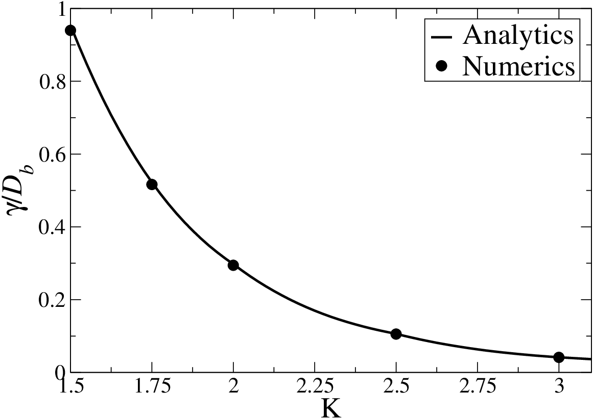
Fig. S4 compares the relaxation rate obtained numerically from the long time tail of the time-evolution and compares it with γth\gamma_{\rm th}. The agreement is very good and shows that the system thermalizes faster near the critical point.

Refer to caption
Figure S4: The thermalization rate γ\gamma obtained from the long time tail of the time-evolution is found to increase on approaching the critical point at K=3/2K=3/2. The solid line is γth\gamma_{\rm th}.

The kinetic equation is valid as long as the backscattering disorder is a weak perturbation. This is certainly the case when K>3/2K>3/2 where the backscattering disorder is RG irrelevant. For K<3/2K<3/2, the disorder is RG relevant, and the ground state is the localized Bose-glass phase. Thus our treatment cannot be generalized to the case of K=1K=1 which corresponds to the hard-core boson or free fermion limit. This is also apparent when we look at the expressions for the rates at K=1K=1. In particular γth\gamma_{\rm th} at zero temperature and K<1K<1 begins to show infrared divergences because

γth​(Teq=0)∼∫1∞d​τ​1τ2​K−1\displaystyle\gamma_{\rm th}(T_{\rm eq}=0)\sim\int_{1}^{\infty}d\tau\frac{1}{\tau^{2K-1}} (S67)

above, as KK is decreased, the first sign of a breakdown of perturbation theory occurs at K=1K=1 when the integral has a logarithmic singularity.

III Estimation of equilibrium temperature TeqT_{\rm eq} from energy conservation

To estimate the energy Δ​E\Delta E injected due to the quench from HiH_{i} to HfH_{f}, we need to evaluate

Δ​E=⟨ψi|Hf|ψi⟩−Egs,f\displaystyle\Delta E=\langle\psi_{i}|H_{f}|\psi_{i}\rangle-E_{{\rm gs},f} (S68)

where Egs,fE_{{\rm gs},f} is the ground-state energy of the final Hamiltonian, while the initial state |ψi⟩|\psi_{i}\rangle is the ground state of HiH_{i}.

Due to symmetry, the expectation value of the backward scattering potential in the initial state vanishes. The remaining part of the Hamiltonian (containing interactions and forward scattering disorder) may be diagonalized exactly as follows,

Hf​0+Vdis,f=∑p≠0u​|p|​Γp†​Γp\displaystyle H_{f0}+V_{{\rm dis},f}=\sum_{p\neq 0}u|p|\Gamma_{p}^{\dagger}\Gamma_{p} (S69)

where

Γp=ap+η~pu​|p|\displaystyle\Gamma_{p}=a_{p}+\frac{\tilde{\eta}_{p}}{u|p|} (S70)
Γp†=ap†+η~p∗u​|p|\displaystyle\Gamma_{p}^{\dagger}=a_{p}^{\dagger}+\frac{\tilde{\eta}_{p}^{*}}{u|p|} (S71)

with

η~p=KLL​|p|2​πe−α|p|/2∫dxη(x)e−i​p​x\displaystyle\tilde{\eta}_{p}=\frac{\sqrt{K}}{L}\sqrt{\frac{L|p|}{2\pi}}e^{-\alpha|p|/2}\int dx\eta(x)e^{-ipx} (S72)

Thus,

⟨ψi|Hf|ψi⟩=∑pu​|p|​⟨ψi|Γp†​Γp|ψi⟩\displaystyle\langle\psi_{i}|H_{f}|\psi_{i}\rangle=\sum_{p}u|p|\langle\psi_{i}|\Gamma_{p}^{\dagger}\Gamma_{p}|\psi_{i}\rangle
=∑pu​|p|​⟨ψi|​(ap†+η~p∗u​|p|)​(ap+η~pu​|p|)​|ψi⟩\displaystyle=\sum_{p}u|p|\langle\psi_{i}|\left(a_{p}^{\dagger}+\frac{\tilde{\eta}^{*}_{p}}{u|p|}\right)\left(a_{p}+\frac{\tilde{\eta}_{p}}{u|p|}\right)|\psi_{i}\rangle
=K​Df2​π​u​∑pe−α​|p|\displaystyle=\frac{KD_{f}}{2\pi u}\sum_{p}e^{-\alpha|p|} (S73)

where we have performed a disorder averaging in the last step. Thus,

⟨ψi|Hf|ψi⟩/L=(1π​α)​K​Df2​π​u\displaystyle\langle\psi_{i}|H_{f}|\psi_{i}\rangle/L=\left(\frac{1}{\pi\alpha}\right)\frac{KD_{f}}{2\pi u} (S74)

Now we estimate the ground state energy of the final Hamiltonian perturbatively in the backward scattering disorder. Using,

e−β​Ω=Tr⁡[e−β​Hf]\displaystyle e^{-\beta\Omega}={\rm Tr}\left[e^{-\beta H_{f}}\right] (S75)

at zero temperature (β−1=0\beta^{-1}=0),

Egs,f=⟨Hf⟩=Ω=−1β​ln⁡[Tr​e−β​Hf]\displaystyle E_{{\rm gs},f}=\langle H_{f}\rangle=\Omega=-\frac{1}{\beta}\ln\left[{\rm Tr}e^{-\beta H_{f}}\right]
=−1βln[Tre−β​H0Tτe−∫0βdτ1V(τ1)]\displaystyle=-\frac{1}{\beta}\ln\left[{\rm Tr}e^{-\beta H_{0}}T_{\tau}e^{-\int_{0}^{\beta}d\tau_{1}V(\tau_{1})}\right]
≃−1β​ln⁡(Tr⁡[e−β​H0])\displaystyle\simeq-\frac{1}{\beta}\ln\left({\rm Tr}\left[e^{-\beta H_{0}}\right]\right)
−1β​ln⁡(1+12​∫0βd​τ1​∫0βd​τ2​T​⟨V⁡(τ1)​V​(τ2)⟩conn)\displaystyle-\frac{1}{\beta}\ln\left(1+\frac{1}{2}\int_{0}^{\beta}d\tau_{1}\int_{0}^{\beta}d\tau_{2}T\langle V(\tau_{1})V(\tau_{2})\rangle_{\rm conn}\right)
=Ω0−12​β​∫0βd​τ1​∫0βd​τ2​T​⟨V⁡(τ1)​V​(τ2)⟩conn\displaystyle=\Omega_{0}-\frac{1}{2\beta}\int_{0}^{\beta}d\tau_{1}\int_{0}^{\beta}d\tau_{2}T\langle V(\tau_{1})V(\tau_{2})\rangle_{\rm conn} (S76)

Since Ω0=0\Omega_{0}=0, after disorder averaging one obtains,

Egs,f=−2LDb∫0∞dτT⟨e2​i​ϕ​(0,τ)e−2​i​ϕ​(0,0)⟩\displaystyle E_{{\rm gs},f}=-2LD_{b}\int_{0}^{\infty}d\tau T\langle e^{2i\phi(0,\tau)}e^{-2i\phi(0,0)}\rangle
=−2LDb∫0∞dτ(11+τ2)K\displaystyle=-2LD_{b}\int_{0}^{\infty}d\tau\left(\frac{1}{1+\tau^{2}}\right)^{K}
=−2​L​Db​π2​Γ⁡(K−12)Γ⁡(K)\displaystyle=-2LD_{b}\frac{\sqrt{\pi}}{2}\frac{\Gamma(K-\frac{1}{2})}{\Gamma(K)} (S77)

Thus the energy per unit length injected due to the quench is

Δ​EL=(1π​α)​K​Df2​π​u+Db​π​Γ⁡(K−12)Γ⁡(K)\displaystyle\frac{\Delta E}{L}=\left(\frac{1}{\pi\alpha}\right)\frac{KD_{f}}{2\pi u}+D_{b}\sqrt{\pi}\frac{\Gamma(K-\frac{1}{2})}{\Gamma(K)} (S78)

The equilibrium temperature TeqT_{\rm eq} is defined by

Δ​EL=1L​∑pe−α​|p|​u​|p|​1eu​|p|/Teq−1\displaystyle\frac{\Delta E}{L}=\frac{1}{L}\sum_{p}e^{-\alpha|p|}u|p|\frac{1}{e^{u|p|/T_{\rm eq}}-1}
=uπ​α2​(Teq​αu)2​ζ​[2,1+Teq​αu]\displaystyle=\frac{u}{\pi\alpha^{2}}\left(\frac{T_{\rm eq}\alpha}{u}\right)^{2}\zeta\left[2,1+\frac{T_{\rm eq}\alpha}{u}\right]
→T¯eq≪1(u​πα2)​T¯eq26\displaystyle\xrightarrow{\bar{T}_{\rm eq}\ll 1}\left(\frac{u\pi}{\alpha^{2}}\right)\frac{\bar{T}_{\rm eq}^{2}}{6} (S79)
→T¯eq≫1(uπ​α2)​T¯eq\displaystyle\xrightarrow{\bar{T}_{\rm eq}\gg 1}\left(\frac{u}{\pi\alpha^{2}}\right)\bar{T}_{\rm eq} (S80)

where T¯eq\bar{T}_{\rm eq} is in units of the cut-off Λ=u/α\Lambda=u/\alpha and ζ\zeta is the Hurwitz Zeta function.

IV Perturbative time-evolution of the density at short times

Note that the kinetic equation is not valid at very short times after the quench due to the leading order gradient expansion which neglects some initial quantum memory effects. The kinetic equation is accurate only at sufficiently long times. In order to smoothly match the short time quantum dynamics with the long time dynamics of the kinetic equation, we use perturbation theory to evolve the density forward for a short time, and use this density as the initial condition for the kinetic equation. Here we outline the results of this perturbation theory.

We plan to study perturbatively the following quantity,

np​(t)=⟨ψi|ei​Hf​t​Γp†​Γp​e−i​Hf​t|ψi⟩\displaystyle n_{p}(t)=\langle\psi_{i}|e^{iH_{f}t}\Gamma_{p}^{\dagger}\Gamma_{p}e^{-iH_{f}t}|\psi_{i}\rangle (S81)

Writing Hf=H0​ff+Vdis,bH_{f}=H_{0f}^{f}+V_{{\rm dis},b} where H0​ff=∑pu​|p|​Γp†​ΓpH_{0f}^{f}=\sum_{p}u|p|\Gamma_{p}^{\dagger}\Gamma_{p} is the Luttinger model with forward scattering disorder, and Vdis,bV_{{\rm dis},b} contains the backward scattering disorder,

np​(t)=⟨ψi|​T~​ei​∫0td​t′​Vdis,b​(t′)​ei​Hf​0f​t​Γp†​Γp​e−i​Hf​0f​t\displaystyle n_{p}(t)=\langle\psi_{i}|\tilde{T}e^{i\int_{0}^{t}dt^{\prime}V_{{\rm dis},b}(t^{\prime})}e^{iH_{f0}^{f}t}\Gamma_{p}^{\dagger}\Gamma_{p}e^{-iH_{f0}^{f}t}
×Te−i∫0tdt′Vdis,b(t′)|ψi⟩\displaystyle\times Te^{-i\int_{0}^{t}dt^{\prime}V_{{\rm dis},b}(t^{\prime})}|\psi_{i}\rangle
=⟨ψi|T~ei​∫0td​t′​Vdis,b​(t′)Γp†ΓpTe−i∫0tdt′Vdis,b(t′)|ψi⟩\displaystyle=\langle\psi_{i}|\tilde{T}e^{i\int_{0}^{t}dt^{\prime}V_{{\rm dis},b}(t^{\prime})}\Gamma_{p}^{\dagger}\Gamma_{p}Te^{-i\int_{0}^{t}dt^{\prime}V_{{\rm dis},b}(t^{\prime})}|\psi_{i}\rangle
=⟨ψi|T~ei​∫0td​t′​Vdis,b​(t′)ap†apTe−i∫0tdt′Vdis,b(t′)|ψi⟩\displaystyle=\langle\psi_{i}|\tilde{T}e^{i\int_{0}^{t}dt^{\prime}V_{\rm dis,b}(t^{\prime})}a_{p}^{\dagger}a_{p}Te^{-i\int_{0}^{t}dt^{\prime}V_{\rm dis,b}(t^{\prime})}|\psi_{i}\rangle
+|η~p|2u2​p2\displaystyle+\frac{|\tilde{\eta}_{p}|^{2}}{u^{2}p^{2}}
+[η~pu​|p|⟨ψi|T~ei​∫0td​t′​Vdis,b​(t′)ap†Te−i∫0tdt′Vdis,b(t′)|ψi⟩+c.c.]\displaystyle+\left[\frac{\tilde{\eta}_{p}}{u|p|}\langle\psi_{i}|\tilde{T}e^{i\int_{0}^{t}dt^{\prime}V_{\rm dis,b}(t^{\prime})}a_{p}^{\dagger}Te^{-i\int_{0}^{t}dt^{\prime}V_{\rm dis,b}(t^{\prime})}|\psi_{i}\rangle+c.c.\right]

Recall that the ap†,apa_{p}^{\dagger},a_{p} fields diagonalize the clean Luttinger model (Df=Db=0D_{f}=D_{b}=0). In perturbation theory we Taylor expand Te−i∫0tdt′Vdis,b(t′)Te^{-i\int_{0}^{t}dt^{\prime}V_{{\rm dis},b}(t^{\prime})} to second order and perform a disorder average. The last term above does not survive disorder averaging, and to 𝒪⁡(Db){\cal O}(D_{b}), we obtain

np​(t)=npf+⟨ψi|ap†​ap|ψi⟩+npb​(t)\displaystyle n_{p}(t)=n_{p}^{f}+\langle\psi_{i}|a_{p}^{\dagger}a_{p}|\psi_{i}\rangle+n_{p}^{b}(t) (S83)

where

npf=|η~p|2u2​p2¯=K​Df/(2​π​u)u​|p|=Tefffu​|p|\displaystyle n_{p}^{f}=\overline{\frac{|\tilde{\eta}_{p}|^{2}}{u^{2}p^{2}}}=\frac{KD_{f}/(2\pi u)}{u|p|}=\frac{T_{\rm eff}^{f}}{u|p|} (S84)

Since the initial state is the ground state of the clean system ⟨ψi|ap†​ap|ψi⟩=0\langle\psi_{i}|a_{p}^{\dagger}a_{p}|\psi_{i}\rangle=0, and

npb​(t)=∫0td​t1​∫0td​t2​⟨ψi|Vdis,b​(t1)​ap†​ap​Vdis,b​(t2)|ψi⟩¯\displaystyle n_{p}^{b}(t)=\!\!\int_{0}^{t}dt_{1}\int_{0}^{t}dt_{2}\overline{\langle\psi_{i}|V_{\rm dis,b}(t_{1})a_{p}^{\dagger}a_{p}V_{\rm dis,b}(t_{2})|\psi_{i}\rangle}

Since ⟨ψi|Vdis,b​(t1)​ap†​ap​Vdis,b​(t2)|ψi⟩¯\overline{\langle\psi_{i}|V_{\rm dis,b}(t_{1})a_{p}^{\dagger}a_{p}V_{\rm dis,b}(t_{2})|\psi_{i}\rangle} depends only on t1−t2t_{1}-t_{2}, we may Fourier transform it as ⟨ψi|Vdis,b​(t1−t2)​ap†​ap​Vdis,b​(0)|ψi⟩=∫−∞∞d​ω​e−i​ω​(t1−t2)​Jp​(ω)\langle\psi_{i}|V_{\rm dis,b}(t_{1}-t_{2})a_{p}^{\dagger}a_{p}V_{\rm dis,b}(0)|\psi_{i}\rangle=\int_{-\infty}^{\infty}d\omega e^{-i\omega(t_{1}-t_{2})}J_{p}(\omega). Then defining T=(t1+t2)/2,τ=t1−t2T=(t_{1}+t_{2})/2,\tau=t_{1}-t_{2}

npb​(t)=∫0t/2d​T​∫−2​T2​Td​τ​e−i​ω​τ​∫−∞∞d​ω​Jp​(ω)\displaystyle n_{p}^{b}(t)=\int_{0}^{t/2}dT\int_{-2T}^{2T}d\tau e^{-i\omega\tau}\int_{-\infty}^{\infty}d\omega J_{p}(\omega)
+∫t/2tdT∫−2​(t−T)2​(t−T)dτe−i​ω​τ∫−∞∞dωJp(ω)\displaystyle+\int_{t/2}^{t}dT\int_{-2(t-T)}^{2(t-T)}d\tau e^{-i\omega\tau}\int_{-\infty}^{\infty}d\omega J_{p}(\omega) (S86)

The integration over T,τT,\tau may be performed in a straightforward manner to give,

npb​(t)=4​∫−∞∞d​ωω​Jp​(ω)​∫0t/2d​T​sin⁡(2​ω​T)\displaystyle n_{p}^{b}(t)=4\int_{-\infty}^{\infty}\frac{d\omega}{\omega}J_{p}(\omega)\int_{0}^{t/2}dT\sin\left(2\omega T\right)
=4​∫−∞∞d​ωω2​sin2⁡(ω​t2)​Jp​(ω)\displaystyle=4\int_{-\infty}^{\infty}\frac{d\omega}{\omega^{2}}\sin^{2}\left(\frac{\omega t}{2}\right)J_{p}(\omega) (S87)

where,

Jp​(ω)=Db​(2​π​K)​e−α​|p||p|​∫−∞∞d​τ​e−K2​Dfu​|τ|\displaystyle J_{p}(\omega)=D_{b}\left(2\pi K\right)\frac{e^{-\alpha|p|}}{|p|}\int_{-\infty}^{\infty}d\tau e^{-\frac{K^{2}D_{f}}{u}|\tau|}
×[ei​ω​τ−i​u​|p|​τ(11+i​τ)2​K+c.c.]\displaystyle\times\left[e^{i\omega\tau-iu|p|\tau}\left(\frac{1}{1+i\tau}\right)^{2K}+c.c.\right] (S88)

The above gives,

Jp​(ω)≃Db​(4​π​KΛ​|p|)​π⁡(1+s​g​n​(ω−u​|p|))Γ⁡(2​K)\displaystyle J_{p}(\omega)\simeq D_{b}\left(\frac{4\pi K}{\Lambda|p|}\right)\frac{\pi\left(1+sgn(\omega-u|p|)\right)}{\Gamma(2K)}
×e−|ω−u|p||/Λ[|ω−u​|p||Λ]−1+2​K+𝒪(DbDf)\displaystyle\times e^{-|\omega-u|p||/\Lambda}\left[\frac{|\omega-u|p||}{\Lambda}\right]^{-1+2K}+{\cal O}\left(D_{b}D_{f}\right) (S89)

Next we take the limit of p→0p\rightarrow 0 in Jp​(ω)J_{p}(\omega), and also the limit of long times so that sin2⁡(ω​t/2)≃1/2\sin^{2}\left(\omega t/2\right)\simeq 1/2. Then

npb​(t→∞)=Teffbu​|p|\displaystyle n_{p}^{b}(t\rightarrow\infty)=\frac{T_{\rm eff}^{b}}{u|p|} (S90)

where

Teffb=Λ​8​π​K​𝒟b​[Γ⁡(2​K−2)Γ⁡(2​K)]\displaystyle T_{\rm eff}^{b}=\Lambda 8\pi K{\cal D}_{b}\left[\frac{\Gamma(2K-2)}{\Gamma(2K)}\right] (S91)

Thus the density of excited quasiparticles obtained from perturbatively time-evolving the system is

np=Tefff+Teffbu​|p|=Teff,0u​|p|\displaystyle n_{p}=\frac{T_{\rm eff}^{f}+T_{\rm eff}^{b}}{u|p|}=\frac{T_{\rm eff,0}}{u|p|} (S92)

The above will act as the initial condition for our kinetic equation.

Our results here hold as long as perturbation theory in DbD_{b} is valid. This is certainly the case when K>3/2K>3/2, but breaks down when KK becomes too small. In particular it is not valid for K=1K=1 which is apparent in the expression for TeffbT_{\rm eff}^{b} in Eq. (S91) which diverges at this point.