A cautionary note on robust covariance plug-in methods

For a $p$-variate random vector $x=(x_{1},\ldots,x_{p})^{T}$ the covariance matrix, or variance-covariance matrix,

is a fundamental descriptive measure and is one of the cornerstones in the development of multivariate methods. The covariance matrix has a number of important basic properties, for example:

Furthermore, for a random sample $X_{n}=(x_{1},\ldots,x_{n})^{T}$ coming from a $p$-variate normal distribution $N_{p}(\mu,\Sigma)$, the finite sample version of $\mathrm{cov}(x)$, i.e. the sample covariance matrix

is the maximum likelihood estimator for the scatter parameter $\Sigma=\mathrm{cov}(x)$. Also, together with the sample mean vector $\bar{x}$, the sample covariance matrix gives a sufficient summary of the data under the assumption of multivariate normality. Hence any method derived assuming multivariate normality will be based solely on the the sample mean vector and sample covariance matrix.

It is well known though that multivariate methods based on the sample mean and sample covariance matrix are highly non-robust to departures from multivariate normality. Such methods are extremely sensitive to just a single outlier and are highly inefficient at longer tailed distributions. Consequently, a substantial amount of research has been undertaken in an effort to develop robust multivariate methods which are not based on the mean vector and covariance matrix. A common approach for “robustifying” classical multivariate methods based on the sample mean vector and covariance matrix is the “plug-in” method, which means to simply modify the method by replacing the mean vector and covariance matrix with robust estimates of multivariate location and scatter. However, sometimes crucial properties of the covariance matrix are needed in order for a particular multivariate method to be valid, and investigating whether these properties hold for the robust scatter replacement is often not addressed. Typically, scatter matrices are defined so that they satisfy the first two properties in Lemma 1, but not necessarily the other properties.

In this paper, we focus on the third property above and its central role in certain multivariate procedures, in particular in independent components analysis (section 4), in observational regression (section 5) and in graphical modeling (section 6). These cases illustrate why the use of plug-in methods should be done with some caution since not all scatter matrices necessarily satisfy this property. Some counterexamples are given in section 3, where it is it also noted that using symmetrized versions of common robust scatter matrices can make the corresponding plug-in method more meaningful. Some comments on the computational aspects of symmetrization are made in section 7. All computations reported in this paper were done using R 2.15.0 (R Development Core Team, 2012), and relied heavily on the R-packages ICS (Nordhausen et al., 2008), ICSNP (Nordhausen et al., 2012) MASS (Venables & Ripley, 2002) and SpatialNP (Sirkiä et al., 2012). Proofs are reserved for the appendix. To begin, the next section briefly reviews that concepts of scatter matrices, affine equivariance and elliptical distributions, and sets up the notation used in the paper.

Many robust variants of the covariance matrix have been proposed within the statistics literature, with the vast majority of these variants satisfying the following definition of a scatter, or pseudo-covariance, matrix.

A scatter statistic $\hat{V}$ is then one that satisfies the above definition when $F_{x}$ is replaced by the empirical cdf. Scatter statistics which satisfy this definition include M-estimators (Huber, 1981; Maronna, 1976), minimum volume ellipsoids (MVE) and minimum covariance determinant (MCD) estimators (Rousseeuw, 1986), S-estimators (Davies, 1987; Lopuhaä, 1989), $\tau$-estimators (Lopuhaä, 1991), projection based scatter estimators (Donoho & Gasko, 1992; Maronna et al., 1992; Tyler, 1994), re-weighted estimators (Ruiz-Gazen, 1993; Lopuhaä, 1999) and MM-estimates (Tatsuoka & Tyler, 2000; Tyler, 2002).

Definition 1 emphasizes only the first two properties of the covariance matrix noted in Lemma 1, with the other stated properties not necessarily holding for a scatter functional in general. In addition, a scatter statistic cannot be viewed as an estimate of the population covariance matrix, but rather as an estimate of the corresponding scatter functional. For some important distributions, though, a scatter functional and the covariance matrix have a simple relationship. For example, elliptically symmetric distributions are often used to evaluate how well a multivariate statistical method performs outside of the normal family. For such distributions, it is known that if $x$ possesses second moments then $V(F_{x})\propto\mathrm{cov}(x)$. This relationship also holds for a broader class of distributions discussed below. We first recall the definition of elliptical distributions (Bilodeau & Brenner, 1999, see e.g.).

If the density of an elliptical distribution exists, then it can be expressed as

where $\rho(\cdot)$ is a function independent of $\mu$ and $\Gamma$ and $\Gamma=\Omega\Omega^{T}$. We then say that $x\sim E(\rho,\mu,\Gamma)$. (For a symmetric positive definite matrix $S$, the notation $S^{1/2}$ refers to its unique symmetric positive semi-definite square root.) A generalization of the spherical distributions and of the elliptical distributions can be constructed as follows (Oja, 2010, see).

The density $f$ (if it exists) of an exchangeable sign-symmetric $y$ must satisfy the property that $f(y)=f(PJy)$ for any $P$ and $J$. We then denote $x\sim ESS(f,\mu,\Omega)$ if and only if it admits the representation $x\sim\Omega y+\mu$ where $y$ has a exchangeable sign-symmetric distribution with density $f$, $\Omega$ is a full rank $p\times p$ matrix and $\mu$ is a $p$-vector. Note that in this model $\Omega$ is not completely identifiable since $ESS(f,\mu,\Omega)\sim ESS(f,\mu,\Omega^{*}=\Omega PJ)$ for any $P$ and $J$. However, $\Gamma=\Omega\Omega^{T}$ is identifiable since $\Omega^{*}{\Omega^{*}}^{T}=\Omega PJJP^{T}\Omega^{T}=\Omega\Omega^{T}=\Gamma$. On the other hand, unlike the elliptical distributions, the distribution $ESS(f,\mu,\Omega)$ can not be completely determined from $f,\mu$ and $\Gamma$.

Clearly the multivariate normal distributions are special cases of the family of elliptical distributions and the elliptical distributions in turn belong to the family of $ESS$ distributions. In particular, $E(\rho,\mu,\Gamma)\sim ESS(f,\mu,\Gamma^{1/2})$ with $f(y)=\exp\{-\rho(y^{T}y)\}$. The $ESS$ distributions also contain other well studied distributions such as the family of $L_{p}$-norm distributions (Gupta & Song, 1997, see for example). For $x\sim ESS(f,\mu,\Omega)$ in general, or $x\sim E(\rho,\mu,\Gamma)$ in particular, the parameter $\Gamma\propto\mathrm{cov}(x)$ provided $\mathrm{cov}(x)$ exist, with the constant of proportionality being dependent on the function $f$ or the function $\rho$ respectively. To simplify notation, it is hereafter assumed that these functions are standardize so that $\Gamma=\mathrm{cov}(x)$ whenever $x$ which has finite second moments. If the second moments do not exist, then $\Gamma$ still contains information regarding the linear relationship between the components of $x$. The following lemma notes that the relationship between $\Gamma$ and $\mathrm{cov}(x)$ extends to any scatter functional.

For these models, all scatter functionals are proportional and so any consistent scatter statistic is consistent for $\Gamma$ up to a scalar multiple. Consequently, and especially when the function $f$ is not specified for the $ESS(f,\mu,\Omega)$ distribution, the parameter $\Gamma$ is usually only of interest up to proportionality. This motivates considering the broader class of shape functionals as defined below. Lemma 2 also holds when $V$ is taken to be a shape functional.

An example of a shape functional which is not a scatter functional is the distribution-free M-estimate of scatter (Tyler, 1987).

It is worth noting that Tyler et al. (2009) conjecture in their Remark 1 that the $ESS$ distributions are perhaps the largest class of distributions which all scatter or shape matrices are proportional to each other. Outside of this class, different scatter or shape statistics estimate different population quantities. This is not necessarily a bad feature, since as noted by several authors (Tyler et al., 2009; Nordhausen et al., 2011) the comparison of different scatter/shape matrices can be useful in model selection, outlier detection and clustering.

Note that due to Lemma 2, any scatter functional satisfies Lemma 1 under an $ESS$ distribution (although properties 3, 4 and 5 are vacuous for any non-normal elliptical distribution since such distributions do not have any independent components). For general distributions, however, one must check that the scatter functional used in a plug-in method has the properties of the regular covariance matrix needed for the method at hand.

Although a zero covariance between two variable does not imply the variables are independent, the property that independence implies a zero covariance (when the second moments exist) is of fundamental importance when one wishes to view the covariance or correlation as a measure of dependency between variables. It has been pointed out by Oja et al. (2006) that many of the popular robust scatter matrices do not posses the property, but they do not present any concrete counterexample. This somewhat surprising observation is not well known and so in this section we explore it in more detail. Some simple counterexamples are given which not only verify this observation but also demonstrates how large a pseudo-correlation,

can be even when the corresponding variables are independent.

Independent components analysis (ICA) has become increasingly popular in signal processing and biomedical applications, where it is viewed as a practical replacement for principal components analysis (PCA). ICA, in its most basic form, presumes that an observable random $p$-vector $x$ is a linear mixture of a latent random $p$-vector $s$, with the components of $s$ being mutually independent. Hence, the ICA model is commonly given as

where $A$ is a full rank mixing matrix. In order for the model to be identifiable, the signal $s$ can have at most one normally distributed component. Even then, the mixing matrix $A$ and signal $s$ are not completely identifiable, since $x$ can also be represented as $x=A_{o}s_{o}$ where $s_{o}=PDs$ and $A_{o}=AD^{-1}P^{T}$, with $P$ being a permutation matrix and $D$ being a full rank diagonal matrix. This, though, is the only indeterminacy in the model. The primary goal in independent components analysis (ICA) is to then find an unmixing matrix $W$ such that $Wx$ has independent components. Consequently, for some permutation matrix $P$ and full rank diagonal matrix D, $W=A_{o}^{-1}$ and $Wx=s_{o}$. A general overview of ICA can be found, for example, in the often cited ICA book by Hyvärinen et al. (2001).

Most approaches to ICA typically begin by first whitening the data using the sample covariance matrix. This is based on the observation that

where $O$ is an orthogonal matrix whenever $s$ is viewed as a standardized signal, i.e. $\mathrm{cov}(s)=I_{p}$. After whitening the data, attention can then be focused on methods for rotating the uncorrelated components of $y$ to obtain independent components. The approach of course presumes that $x$ possesses second moments. An obvious, though naive, way to make this approach more robust would be to simply replace $\mathrm{cov}(x)$ with some robust scatter matrix $V(x)$. This is proposed, for example, by (Hyvärinen et al., 2001, Section 14.3.2), and by Baloch et al. (2005), who recommend using the minimum covariance determinant (MCD) estimator. However, in neither case is it noted that for such an approach to be valid either the signal $s$ must have a symmetric distribution, or more exactly to have at most one skewed component, or the robust covariance must satisfy the independence property (5), which e.g. is not satisfied by the MCD. Problems in practice, when simply replacing the regular covariance matrix with the MCD in the context of the popular fastICA method, have been noted by Brys et al. (2005). The reason such problems can arise is that if $V(x)$ does not satisfy (5), then $V(s)$ is not necessarily diagonal and hence the signal may not correspond to any rotation of $y=V(x)^{-1/2}x$.

To quantitatively demonstrate the relevance of the independence property, we consider the bivariate case where $s$ has two skew independent components, the first component having a $\chi_{1}^{2}$ distribution and the second component having a $\chi_{2}^{2}$ distribution, with both components being standardized to have mean zero and unit variance. For this example, we use the ICA method proposed by Oja et al. (2006). This ICA method requires two scatter (or shape) matrices, say $V_{1}$ and $V_{2}$, with both satisfying the independence property. The method consists of using $V_{1}(x)$ to first whiten the data, giving $y=V_{1}(x)^{-1/2}x$, and then performing a principal component analysis on $V_{2}(y)$. The resulting principal components of $y$ then correspond to the independent components. The results are also the same when the roles of $V_{1}$ and $V_{2}$ are interchanged. For more details, see Oja et al. (2006).

A small simulation study was conducted using samples of size 1000 and with 1000 replications. Since this ICA method is affine invariant, the choice of the mixing matrix $A$ has no effect on the performance of the method, and so without loss of generality we take $A=I$. Using the terminology established in the earlier sections, we consider the following pairs of scatter matrices (i) $\mathrm{cov}$-$\mathrm{cov}4$ (ii) $V_{CAU}$-$\mathrm{cov}$, (iii) $V_{sCAU}$-$\mathrm{cov}$, (iv) $V_{TYL}$-$V_{HUB}$, and (v) $V_{sTYL}$-$V_{sHUB}$. Case (iii) and (v) are the symmetrized version of (ii) and (iv) respectively. Case (i) is already the same as its symmetrized version, and it corresponds to the classical FOBI method (Cardoso, 1989). Note that only for the cases (i), (iii) and (v) do both scatter matrices satisfy the independence property. To measure the performance of the methods, we use the minimum distance index MD, proposed in (Ilmonen et al., 2010), which is defined to be

where $P$ is a permutation matrix and $D$ a diagonal matrix with non-zero entries. The range of the index is $[0,1]$, with 0 corresponding to an optimal recovery of the independent components. Box-plots for the simulations are shown in Figure 3. The plots clearly show the relevance of the independence property here when there is more than one asymmetric component, even in case (ii) which consists on only one scatter matrix without the independence property.

In this section we consider observation multivariate linear regression, that is linear regression for the case when the explanatory variables, as well as the responses, are randomly observed rather than controlled. The classical multivariate linear regression model is then

where $y$ is a $q$-dimensional response, $x$ is a $p$-vector of explanatory variables with distribution $F_{x}$, and $\epsilon\in\Re^{q}$ is a random error term, independent of $x$, with distribution $F_{\epsilon}$. In this setting, interest usually is focused still on estimating the intercept vector $\alpha\in\Re^{p}$, the $p\times q$ slope matrix $\mathcal{B}$ and perhaps the error variance-covariance matrix $\mathrm{cov}(\epsilon)=\Sigma_{\epsilon\epsilon}$ if it exists.

The standard least squares approach is well known to be highly non-robust, and so there have been numerous proposed robust regression methods. One such method is based on the observation that if both $x$ and $\epsilon$ possess second moments, and if $\mathrm{E}(\epsilon)=0$, then

which corresponds to the population or functional version of the estimates arising from the least squares method. One can then generate a robust functional version by again simply replacing the first two moments with robust versions of scatter and location. That is, let $z=(x^{T},y^{T})^{T}$, which concatenates $x$ and $y$, and consider the corresponding partitions of an affine equivariant location functional $\mu(z)$ and a scatter functional $V(z)$,

If the distribution of $\epsilon$ is symmetric, then it has been observed in Croux et al. (2003) that the parameters $\alpha$ and $\mathcal{B}$ can also be identified, even if no moments exist, through the equations

and so using the finite sample versions of $\mu(z)$ and $V(z)$ in the above relationship gives, under general regularity conditions, consistent estimates of $\mathcal{B}$ and $\alpha$.

This approach was first proposed for univariate multiple regression by Maronna & Morgenthaler (1986) using $M$-estimators of multivariate location an scatter. They note that this approach, unlike $M$-estimates of regression, yields bounded influence regression estimates. This approach has also been studied for the Oja sign covariance matrix in Ollila et al. (2002), for the Lift Rank Covariance Matrix in Ollila et al. (2003), for S-estimators in Croux et al. (2003) and for the MCD in Rousseeuw et al. (2004).

The error variance $\Sigma_{\epsilon\epsilon}$ is not a robust functional itself, and is not identifiable when the error term does not have second moments. Consequently, it is usually replaced by a robust scatter matrix for the residual term. Also, if $\epsilon$ does not have a symmetric distribution, then the intercept term $\alpha$ is confounded with the location of the error term (Hettmansperger & McKean, 2011, Chapter 3 of). It has not been previously noted, though, how the relationship $\mathcal{B}=V_{xx}^{-1}V_{xy}$ is affected by asymmetric error distributions. We first note that, due to the affine equivariance property of a scatter (or shape) functional $V(z)$, this relationship always yields the proper equivariance properties for the slope parameters.

Despite these equivariance properties, in order to obtain $B(x,y)=\mathcal{B}$, additional conditions on $V(z)$ are needed, which as shown by corollary 1, holds for symmetrized scatter/shape matrices.

In order to demonstrate the necessity of symmetrization here whenever skewness is present in both $x$ and $\epsilon$, we conducted a simulation study for the model

where $x$ has a log-normal distribution with shape parameter $\sigma=1$ standardized such that $E(x)=0$ and $\mathrm{var}(x)=1$ and $\epsilon$ has an exponential distribution standardized to have $E(\epsilon)=0$ and $\mathrm{var}(\epsilon)=1$. For samples of size 2000, $\beta$ is estimated using (i) the regular covariance matrix $\mathrm{cov}$, (ii) M-estimator derived from as the maximum likelihood estimator of an elliptical Cauchy distribution $V_{CAU}$, (iii) the symmetrized version of $V_{sCAU}$ , (iv) the M-estimator using Huber’s weights $V_{HUB}$, (v) the symmetrized version of $V_{sHUB}$, (vi) Tyler’s shape matrix $V_{TYL}$, (vii) the symmetrized version of $V_{sTYL}$, (viii) the minimum volume estimator $V_{MVE}$ and (ix) the minimum determinant estimator $V_{MCD}$. The results, based on 1000 replications and presented in Figure 4, shows the severe bias when non-symmetrized scatter matrices are used.

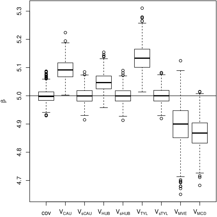
which clearly shows that in this case the estimate for $\beta$ is severely biased when non-symmetrized scatter matrices are used.

The last method considered in this paper is graphical modeling for quantitative variables based on undirected graphs. In graphical models, one is usually interested in those pairs of variables which are independent conditional on all the other variables, or, in graphical modeling terminology, one is interested in those vertices (variables) which have no edges between them. In general, finding conditionally independent variables is challenging and so finding variables with zero partial correlations often serves as a proxy. In this section, we investigate the relationship between conditional independence and robust versions of the partial correlation.

For $p\geq 3$ random variables, consider the relationship between the variables $u$ and $v$ given $x$, with $x$ containing the remaining $p-2$ variables. Denoting $y=(u,v)^{T}$, the partial variance-covariance matrix of $y$ given $x$ is given by

where $\Sigma_{yy\cdot x}=\mathrm{cov}(y)-\mathrm{cov}(y,x)\mathrm{cov}(x)^{-1}\mathrm{cov}(x,y)$, which corresponds to the covariance matrix of the residuals between the orthogonal projections of $u$ and $v$ onto the $p-2$-dimensional subspace spanned by $x$. The corresponding partial correlation between $u$ and $v$ given $x$ is then simply

The partial correlation can also be expressed in terms of the precision or concentration matrix of the combined vector $z=(y^{T},x^{T})^{T}$. Specifically, expressing the precision or concentration matrix of $z$ as $\Sigma_{z}^{-1}=\{\sigma^{ij}_{z}\}$, for $i,j=1,\ldots,p$, where $\Sigma_{z}=\mathrm{cov}(z)$, one obtains

and hence $\rho_{12\cdot x}=0$ if and only if $\sigma_{z}^{12}=0$.

For Gaussian graphical models, for which $z$ is presumed to be multivariate normal, conditional independence between $u$ and $v$ given $x$, i.e. $u\perp v\mid x$, is equivalent to the partial correlation $\rho_{12\cdot x}=0$. In general, conditional independence implies a conditional correlation of zero, presuming the second moments exist, although the converse does not hold in general. However, a perhaps lesser known result is that conditional independence does not imply a zero partial correlation in general. Some additional conditions are needed. In particular, if the regression of $y$ on $x$ is linear, then conditional independence implies a zero partial correlation, see Theorem 1 in Baba et al. (2004). Under such conditions, variables having zero partial correlations then serve as candidates for conditionally independent variables. When used in place of conditional independence, zero partial correlations help provide a parsimonious understanding of the relationship between variables.

Robustness issues have been considered for graphical models, see for example Finegold & Drton (2011) and Vogel & Fried (2011). In both papers, the emphasis is on finding pairs of variables for which a robust version of the partial correlations are zero. The approach used in Finegold & Drton (2011) is a robust graphical lasso. The method uses a penalized maximum likelihood approach based on an elliptical $t$-distribution. The approach advocated in Vogel & Fried (2011) is a plug-in method based on using robust scatter matrices. They also study the asymptotic properties of the plug-in method under elliptical distributions. Consequently, neither paper addresses conditional independence since conditional independence can never hold for variables following a joint elliptical distribution other than the multivariate normal.

Outside the elliptical family, an important question worth addressing is under what conditions does conditional independence imply that the the plug-in version of the partial correlation equals zero? Since regression, i.e. the conditional mean of $y$ given $x$, is itself not a robust concept and also is naturally related to covariances, the condition that regression be linear is not helpful here. We leave general conditions under which conditional independence implies a zero robust partial correlation as an open question. We can, though, obtain results for the following model

where $A$ is a non-random $2\times(p-2)$ matrix, $\epsilon=(\epsilon_{u},\epsilon_{v})^{T}$, and $x$, $\epsilon_{u}$ and $\epsilon_{v}$ are mutually independent. For this model, it readily follows that $u\perp v\mid x$. Also, if the first moments exist then the regression of $y$ on $x$ is linear. Again, if one uses symmetrized scatter matrices than one obtains a plug-in version of the partial correlation which is equal to zero under this model.

As an example for illustrating Theorem 4, consider the simple graphical model given in Figure 5, where $u=4x+\epsilon_{1}$ and $v=5x+\epsilon_{2}$, with $x$ having a standard normal distribution, $\epsilon_{1}$ a log-normal distribution with shape parameter $\sigma=1$ standardized such that $E(\epsilon_{1})=0$ and $\mathrm{var}(\epsilon_{1})=1$ and $\epsilon_{2}$ a $\chi^{2}_{1}$ distribution standardized to have $E(\epsilon_{2})=0$ and $\mathrm{var}(\epsilon_{2})=1$. Using the same nine scatter matrices (i)-(ix) as in the previous section, box plots for the plug-in partial correlation of $u$ and $v$ given $x$ for sample of size 2000 based on 1000 replications are presented in Figure 6. Again, the advantage to using symmetrized scatter/shape matrices is clearly shown.

For various robust multivariate plug-in methods, we recommend symmetrized scatter matrices since they help protect against severe bias whenever skew components are present. A drawback to using symmetrized scatter matrices, though, is that they are more computationally intensive than their non-symmetrized counterparts. For a sample of size $n$, a symmetrized scatter matrix involves $n^{2}$ pairs. On the other hand, it does not require an estimate of location since the difference is centered at the origin. Consequently, only those pairwise differences $x_{i}-x_{j}$ for which $i>j$ are required for its computation and so the number of pairwise differences needed reduces somewhat to $n(n-1)/2$. Modern computers, though, have become so powerful that computational cost should not deter the use of symmetrized scatter matrices when appropriate. Unfortunately, most robust scatter matrices implemented in packages such as R do not allow the option of specifying the location vector, and so cannot be applied readily in computing symmetrized scatter matrices. We hope the discussion in this paper will motivate future implementations of scatter matrices to include a fixed location option, as is the case in the R packages ICS and ICSNP.

It may be difficult in general to develop algorithms which spread the computation of a scatter matrix over several cores. For $M$-estimates of scatter, though, parallelization is possible. To see this, we note that when computing a symmetrized $M$-estimate of scatter $V_{sym}$ via the simple iteratively weighted least squares algorithm, the update step is given by

where $V_{sym,k}$ is the current value of the scatter matrix and $w(\cdot)$ is the weight function associated with the $M$-estimate. A simple way to compute the symmetrized scatter matrix $V_{sym}$ which allows parallelization is to then set

and so the iteration update for the symmetrized version becomes

To illustrate computation times, we considered the symmetrized version of Tyler’s shape matrix $V_{sTYL}$, i.e. Dümbgen’s shape matrix, implemented as duembgen.shape in the R-package ICSNP and the symmetrized $M$-estimator of scatter using Huber’s weights $V_{sHUB}$ implemented as symm.huber in the R-package SpatialNP. The average computing times out of 5 runs for $N_{p}(0,\Sigma)$ data, where $\Sigma$ was randomly chosen, computed on a Intel(R) Xeon(R) CPU X5650 with 2.67GHz and 24GB of memory running a 64-bit RedHat Linux are presented in Figure 7. The figure shows that the computation time as of function of sample size is close to linear when plotted on a log-log scale with a slope of approximately 2. Hence, the computation times are approximately of the order $n^{2}$. Also, for samples of size $n=500$ the computation times tend to be around one second, and that the symmetrized $M$-estimates are computationally feasible for even fairly large sample sizes. As a comparison, for $p=10$, computation times for the non-symmetrized version of the M-estimators are also shown in the figure.

The goal of this paper has been to stress that some important or “good” properties of the covariance matrix do not necessarily carry over to affine equivariant scatter matrices. Consequently, it is necessary to exercise some caution when implementing robust multivariate procedures based on the plug-in method, i.e. when substituting a robust scatter matrix for the covariance matrix in classical multivariate procedures. In particular, the validity of some important multivariate methods require that the scatter matrix satisfy certain independence properties, which do not necessarily hold whenever the components arise from a skewed distribution. Thus, we recommended the use of symmetrized scatter matrices in such situations, since they are the only known scatter matrices which satisfy the independence property, Definition 5, or the block independence property, Definition 7. We further conjecture that the only scatter matrices that satisfy these independence properties are those which can be expressed in terms of the pairwise differences of the observation.

This paper has focused on the independence properties of scatter matrices. It would also be worth considering which scatter matrices, if any, possess the additivity property of the covariance matrix, Lemma 1.4. This property is relevant in factor analysis, in structural equation modeling, and in other multivariate methods. For example, the factor analysis model is given by

where $f$ corresponds to $k<p$ latent factors and $\epsilon$ corresponds to a $p$-variate error term. $\epsilon$. The parameter $\mu$ represents a $p$-variate location and $\Lambda$ corresponds to the $p\times k$ matrix of factor loadings (defined up to an orthogonal transformation). The standard factor analysis assumptions are that the components of both $f$ are $\epsilon$ are mutually independent, and that $f$ and $\epsilon$ are also independent of each other. Furthermore, if the first two moments exist, then is further assumed without loss of generality that $E(f)=0$, $\mathrm{cov}(f)=I_{k}$, $E(\epsilon)=0$ and $\mathrm{cov}(\epsilon)=D$, where $D$ is a diagonal matrix with positive entries. Consequently, one can view such as factor analysis model as a reduced rank covariance model with an additive diagonal term, i.e. as

This decomposition is central to the classical statistical methods in factor analysis. It is not clear though if one can define other scatter matrices so that

with both $V(f)$ and $V(\epsilon)$ being diagonal. Some robust plug-in methods for factor analysis and structural equation models have been considered by Pison et al. (2003) and Yuan & Bentler (1998).

Let $J$ again represents a sign-change matrix, that is a diagonal matrix with diagonal elements of either $\pm 1$. Also, let $P$ represent a permutation matrix obtained by permuting the rows and or columns of $I_{p}$.

References

- Baba et al. (2004) Baba, K., Shibata, R. & Sibuya, M. (2004). Partial correlation and conditional correlation as measures of conditional independence. Australian & New Zealand Journal of Statistics 46, 657–664.
- Baloch et al. (2005) Baloch, S. H., Krim, H. & Genton, M. G. (2005). Robust independent component analysis. In Proceedings of the 2005 IEEE/SP 13th Workshop on Statistical Signal Processing.
- Bilodeau & Brenner (1999) Bilodeau, M. & Brenner, D. (1999). Theory of Multivariate Statistics. New York: Springer-Verag.
- Brys et al. (2005) Brys, G., Hubert, M. & Rousseeuw, J. (2005). A robustification of independent component analysis. Journal of Chemometrics 19, 364–375.
- Cardoso (1989) Cardoso, J.-F. (1989). Sources separation using higher moments. In Proceedings of the 2000 IEEE International conference on Acoustics, Speech and Signal Processing.
- Croux et al. (2003) Croux, C., Van Aelst, S. & Dehon, C. (2003). Bounded influence regression using high breakdown scatter matrices. Annals of the Institute of Mathematical Statistics 55, 265–285.
- Davies (1987) Davies, P. L. (1987). Asymptotic behavior of S-estimates of multivariate location parameters and dispersion matrices. Annals of Statistics 15, 1269–1292.
- Donoho & Gasko (1992) Donoho, D. L. & Gasko, M. (1992). Breakdown properties of location estimates based on halfspace depth and projected outlyingness. Annals of Statistics 20, 1803–1827.
- Dümbgen (1998) Dümbgen, L. (1998). On Tyler’s -functional of scatter in high dimension. Annals of the Institute of Statistical Mathematics 50, 471–491.
- Finegold & Drton (2011) Finegold, M. & Drton, M. (2011). Robust graphical modeling of gene networks using classical and alternative t-distributions. The Annals of Applied Statistics 5, 1057–1080.
- Gupta & Song (1997) Gupta, A. K. & Song, D. (1997). Lp-norm spherical distribution. Journal of Statistical Planning and Inference 60, 241–260.
- Hettmansperger & McKean (2011) Hettmansperger, T. & McKean, J. (2011). Robust Nonparametric Statistical Methods. Boca Raton: CRC Press, 2nd ed.
- Huber (1981) Huber, P. J. (1981). Robust Statistics. New York: Wiley.
- Hyvärinen et al. (2001) Hyvärinen, A., Karhunen, J. & Oja, E. (2001). Independent component analysis. New York: Wiley & Sons.
- Ilmonen et al. (2010) Ilmonen, P., Nordhausen, K., Oja, H. & Ollila, E. (2010). A new performance index for ICA: Properties, computation and asymptotic analysis. In Latent Variable Analysis and Signal Separation, V. Vigneron, V. Zarzoso, E. Moreau, R. Gribonval & E. Vincent, eds. Heidelberg: Springer, pp. 229–236.
- Kent & Tyler (1991) Kent, J. T. & Tyler, D. E. (1991). Redescending -estimates of multivariate location and scatter. The Annals of Statistics 19, 2102–2119.
- Lopuhaä (1989) Lopuhaä, H. P. (1989). On the relation between S-estimators and M-estimators of multivariate location and covariance. Annals of Statistics 17, 1662–1683.
- Lopuhaä (1991) Lopuhaä, H. P. (1991). Multivariate -estimators for location and scatter. Canadian Journal of Statistics 19, 307–321.
- Lopuhaä (1999) Lopuhaä, H. P. (1999). Asymptotics of reweighted estimators of multivariate location and scatter. Annals of Statistics 27, 1638––1665.
- Maronna & Morgenthaler (1986) Maronna, R. & Morgenthaler, S. (1986). Robust regression through robust covariances. Communications in Statistics, Theory and Methods 15, 1347–1365.
- Maronna (1976) Maronna, R. A. (1976). Robust M-estimators of multivariate location and scatter. Annals of Statistics 4, 51–67.
- Maronna et al. (2006) Maronna, R. A., Martin, R. D. & Yohai, V. J. (2006). Robust Statistics - Theory and Methods. Chichester, UK: John Wiley & Sons.
- Maronna et al. (1992) Maronna, R. A., Stahel, W. A. & Yohai, V. J. (1992). Bias-robust estimators of multivariate scatter based on projections. Journal of Multivariate Analysis 42, 141–161.
- Nordhausen & Oja (2011) Nordhausen, K. & Oja, H. (2011). Scatter matrices with independent block property and ISA. In Proceedings of the 19th European Signal Processing Conference 2011 (EUSIPCO 2011).
- Nordhausen et al. (2011) Nordhausen, K., Oja, H. & Ollila, E. (2011). Multivariate models and the first four moments. In Nonparametric Statistics and Mixture Models: A Festschrift in Honor of Thomas P. Hettmansperger, D. Hunter, D. Richards & J. Rosenberger, eds. Singapore: World Scientific, pp. 267–287.
- Nordhausen et al. (2008) Nordhausen, K., Oja, H. & Tyler, D. E. (2008). Tools for exploring multivariate data: The package ICS. Journal of Statistical Software 28, 1–31.
- Nordhausen et al. (2012) Nordhausen, K., Sirkia, S., Oja, H. & Tyler, D. E. (2012). ICSNP: Tools for Multivariate Nonparametrics. R package version 1.0-9.
- Oja (2010) Oja, H. (2010). Multivariate Nonparametric Methods with R: An Approach Based on Spatial Signs and Ranks. New York: Springer.
- Oja et al. (2006) Oja, H., Sirkiä, S. & Eriksson, J. (2006). Scatter matrices and independent component analysis. Austrian Journal of Statistics 35, 175–189.
- Ollila et al. (2002) Ollila, E., Oja, H. & Hettmansperger, T. P. (2002). Estimates of regression coefficients based on the sign covariance matrix. Journal of the Royal Statistical Society: Series B (Statistical Methodology) 64, 447–466.
- Ollila et al. (2003) Ollila, E., Oja, H. & Koivunen, V. (2003). Estimates of regression coefficients based on lift rank covariance matrix. Journal of the American Statistical Association 98, 90–98.
- Pison et al. (2003) Pison, G., Rousseeuw, P. J., Filzmoser, P. & Croux, C. (2003). Robust factor analysis. Journal of Multivariate Analysis 84, 145–172.
- R Development Core Team (2012) R Development Core Team (2012). R: A Language and Environment for Statistical Computing. R Foundation for Statistical Computing, Vienna, Austria. ISBN 3-900051-07-0.
- Roelant et al. (2009) Roelant, E., Van Aelst, S. & Croux, C. (2009). Multivariate generalized S-estimators. Journal of Multivariate Analysis 100, 876–887.
- Rousseeuw (1986) Rousseeuw, P. J. (1986). Multivariate estimation with high breakdown point. In Mathematical Statistics and Applications, W. Grossman, G. Pflug, I. Vincze & W. Wertz, eds. Dordrecht: Reidel, pp. 283–297.
- Rousseeuw et al. (2004) Rousseeuw, P. J., Van Aelst, S., Van Driessen, K. & Gullo, J. A. (2004). Robust multivariate regression. Technometrics 46, 293–305.
- Ruiz-Gazen (1993) Ruiz-Gazen, A. (1993). Estimation robuste d’une matrice de dispersion et projections révélatrices. Ph.d. dissertation, Université Paul Sabatier, Toulouse.
- Sirkiä et al. (2012) Sirkiä, S., Miettinen, J., Nordhausen, K., Oja, H. & Taskinen, S. (2012). SpatialNP: Multivariate nonparametric methods based on spatial signs and ranks. R package version 1.1-0.
- Sirkiä et al. (2007) Sirkiä, S., Taskinen, S. & Oja, H. (2007). Symmetrised M-estimators of scatter. Journal of Multivariate Analysis 98, 1611–1629.
- Tatsuoka & Tyler (2000) Tatsuoka, K. S. & Tyler, D. E. (2000). On the uniqueness of S-functionals and M-functionals under nonelliptical distributions. Annals of Statistics 28, 1219–1243.
- Tyler (1987) Tyler, D. E. (1987). A distribution-free -estimator of multivariate scatter. The Annals of Statistics 15, 234–251.
- Tyler (1994) Tyler, D. E. (1994). Finite sample breakdown points of projection based multivariate location and scatter statistics. Annals of Statistics 22, 1024–1044.
- Tyler (2002) Tyler, D. E. (2002). High breakdown point multivariate M-estimation. Estadistica 54, 213–247.
- Tyler et al. (2009) Tyler, D. E., Critchley, F., Dümbgen, L. & Oja, H. (2009). Invariant co-ordinate selection. Journal of the Royal Statistical Society B 71, 549–592.
- Venables & Ripley (2002) Venables, W. N. & Ripley, B. D. (2002). Modern Applied Statistics with S. New York: Springer, 4th ed. ISBN 0-387-95457-0.
- Vogel & Fried (2011) Vogel, D. & Fried, R. (2011). Elliptical graphical modelling. Biometrika 98, 935–951.
- Yuan & Bentler (1998) Yuan, K.-H. & Bentler, P. M. (1998). Structural equation modeling with robust covariances. Sociological Methodology 28, 363–396.