Component Substitution through Dynamic ReconfigurationsThanks: This work has been partially funded by the Labex ACTION, ANR-11-LABX-0001-01.

Dynamic reconfigurations [12, 3, 24] increase the availability and the reliability of component-based systems by allowing their architecture to evolve at runtime. In this paper, in addition to dynamic evolution reconfigurations, possibly guided by temporal patterns [13, 22, 14], we consider reconfigurations bringing into play by component substitutions. These reconfigurations by substitution may change the model’s behaviour. The questions we are interested in are: How are such model transformations represented? What aspects of the model’s behaviour can be changed? Can new behaviour be added, can existing behaviours be replaced or combined with new behaviours?

More precisely, in our previous works [13, 22, 14], a component-based framework has been developed: a component-based model with dynamic reconfigurations has been defined and shown consistent, a linear temporal pattern logic allowing expressing properties over sequences of dynamic reconfigurations has been defined. In our work we suppose an interface preservation that encompasses the internal behaviour of the manipulated components. The approaches in [11, 23] allow to deal with such an interface preservation.

Component substitution reconfigurations being motivated by numerous practical applications, this paper proposes to enrich the existing component-based framework with a notion of component substitutability. Figure 1 displays two kinds of reconfigurations: Horizontal reconfigurations represent the dynamic architecture’s evolution whereas vertical substitutions lead to different implementations. As the model and its implementations must remain consistent through evolution, in this paper we study the impact of reconfigurations by substitution (vertical substitutions) on sequences of dynamic reconfigurations (horizontal reconfigurations).

Since our component-based model is formulated as a theory in first order logic (FOL), this is achieved by introducing a new relation over components, and a set of logical constraints. Then, the paper presents a notion of simulation between dynamic reconfigurable systems wrt. a given component substitution relation, and addresses the checking of this relation, which is known to be, in general, undecidable.

Layout of the paper. In Sect. 2 we recall the main features of the architectural reconfiguration model introduced in [13, 22] and illustrate them on an example of the HTTP server. In Sect. 3, a new reconfiguration operation by component substitution is introduced and substitutability constraints are defined to ensure component encapsulation. In Sect. 4 component substitutability is integrated into a substitutability-based simulation relation. This relation being undecidable in general, a semi-algorithm is proposed to evaluate on the fly dynamic reconfiguration sequences and, consequently, the component substitutability-based simulation. Section 5 explains how to use the B tools for dealing with component substitutability through dynamic reconfigurations, and describes experiments on the HTTP server example. Finally, we conclude in Sect. 6.

The (dynamic) reconfigurations we consider here make the component-based architecture evolve dynamically. They are combinations of primitive operations such as instantiation/destruction of components; addition/removal of subcomponents to/from composite ones; binding/unbinding of component interfaces; starting/stopping components; setting parameter values of components. In the remaining of the paper, these primitive operations are not considered, we only focus on their combinations providing example-specific reconfigurations.

In general, system configuration is the specific definition of the elements that define or prescribe what a system is composed of. We define a configuration to be a set of architectural elements (components, required or provided interfaces and parameters) together with relations to structure and to link them, as depicted in Fig. 2 ¹¹ 1 See Definition 5 in Appendix A.

Given a set of configurations $\mathcal{C}=\{c,c_{1},c_{2},\ldots\}$, we introduce a set $CP$ of configuration properties on the architectural elements and the relations between them. These properties are specified using first-order logic formulas. The interpretation of functions, relations, and predicates is done according to basic definitions in [19] and in [14]¹. We now define a configuration interpretation function $l:\mathcal{C}\rightarrow CP$ which gives the largest conjunction of $cp\in CP$ evaluated to true on $c\in\mathcal{C}$ ²² 2 By definition in [19], this conjunction is in $CP$..

Among all the configuration properties, we consider the architectural consistency constraints $CC$ which express requirements on component assembly common to all the component architectures. They allow defining consistent configurations which notably respect the following rules. Their intuition is as follows, together with a formal description for several constraints³³ 3 The whole definition is available at http://www.lina.sciences.univ-nantes.fr/aelos/publications/fesca14.:

• •

  a component supplies one provided interface, at least;

• •

  the composite components do not have any parameters;

• •

  a sub-component must not be a composite including its own parent component;

• •

  two bound interfaces must have the same interface type; they are not supplied by the same component, but their containers are sub-components of the same composite;

  $$\begin{array}[]{l}\forall ip\in ProvInterfaces,\\ \forall ir\in ReqInterfaces\end{array}.\left(Binding(ip)=ir\Rightarrow\begin{array}[]{l}InterfaceType(ip)=InterfaceType(ir)\\ \wedge\ Container(ip)\neq Container(ir)\\ \wedge\ \exists\penalty\ c\in Components.\left(\begin{array}[]{l}(Container(ip),c)\in Parent\\ \wedge(Container(ir),c)\in Parent\\ \end{array}\right)\end{array}\right)$$

• •

  when binding two interfaces, there is a need to ensure that they have not been involved in a delegation yet; similarly, when establishing a delegation link between two interfaces, the specifier must ensure that they have not been involved in a binding yet;

• •

  a provided (resp. required) interface of a sub-component is delegated to at most one provided (resp. required) interface of its parent component; the interfaces involved in the delegation must have the same interface type;

• •

  a component is $started$ only if its mandatory required interfaces are bound or delegated.

Let $\mathcal{R}$ be a finite set of reconfiguration operations. The possible evolutions of the component architecture via the reconfiguration operations are defined as a transition system over $\mathcal{R}$.

Let us write $c\stackrel{{\scriptstyle ope}}{{\rightarrow}}c^{\prime}$ when a target configuration $c^{\prime}$ is reached from a configuration $c$ by a reconfiguration operation $ope\in\mathcal{R}$. Given the model $S=\langle\mathcal{C},\mathcal{C}^{0},\mathcal{R},\rightarrow\rangle$, an evolution path $\sigma$ (or a path for short) in $S$ is a (possibly infinite) sequence of configurations $c_{0},c_{1},c_{2},\ldots$ such that $\forall i\geq\penalty\ 0\penalty\ .\penalty\ (\exists\ ope_{i}\in\mathcal{R}.(c_{i}\stackrel{{\scriptstyle ope_{i}}}{{\rightarrow}}c_{i+1}\in\rightarrow))$. We write $\sigma(i)$ to denote the $i$-th configuration of a path $\sigma$. Let $\Sigma$ denote the set of paths, and $\Sigma^{f}$ ($\subseteq\Sigma$) the set of finite paths.

To illustrate our model, let us consider an example of a HTTP server ⁴⁴ 4 The example specification is available at http://fractal.ow2.org/tutorial.. The architecture of this server is depicted in Fig. 3. The RequestReceiver component reads HTTP requests from the network and transmits them to the RequestHandler component. In order to keep the response time as short as possible, RequestHandler can either use a cache (with the component CacheHandler) or directly transmit the request to the RequestDispatcher component. The number of requests (load) and the percentage of similar requests (deviation) are two parameters defined for the RequestHandler component. The CacheHandler component is used only if the number of similar HTTP requests is high. The memorySize for the CacheHandler component depends on the overall load of the server.

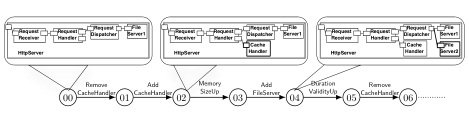
The validityDuration of data in the cache also depends on the overall load of the server. The number of used file servers (like the FileServer1 and FileServer2 components) used by RequestDispatcher depends on the overall load of the server. On this example, the considered reconfiguration operations are:

• •

  AddCacheHandler and RemoveCacheHandler which are used to add and remove CacheHandler;

• •

  AddFileServer and removeFileServer which are used to add and remove FileServer2;

• •

  MemorySizeUp and MemorySizeDown which are used to increase and to decrease the MemorySize value;

• •

  DurationValidityUp and DurationValidityDown which are used to increase and to decrease the ValidityDuration value.

A possible evolution path of the HTTP server architecture is given in Fig. 4.

In this section we enrich our component-based framework with a new kind of reconfigurations allowing a structural substitution of the components with respect to the component encapsulation. We suppose an interface preservation encompassing the internal behaviour of the considering components, i.e. using the same interface implies the same internal component behaviour [11, 23]. We want the substituted component to supply the same interfaces of the same types as before. This way the other components do not see the difference between the component and its new “substituted” version, and thus there is no need to adapt them. As the substitution of a component should not cause any changes outside of this component, only the two following kinds of component substitutions are allowed:

• •

  either a component can be replaced by a new version of itself, or

• •

  a component can be replaced by a composite component which encapsulates new sub-components providing at least the same functionalities as before substitution.

For the allowed substitution cases, Figure 5 displays how the architectural elements and relations are defined at two pre- and post-substitution levels. Let $c_{A}$ and $c_{R}$ be two architectural configurations at respectively a pre-substitution and a post-substitution levels. The substitute reconfiguration is then expressed by a partial function $Subst\,:\,Components_{A}\rightarrow Components_{R}$ that gives how the components are substituted in $c_{A}$ to obtain $c_{R}$.

Let us illustrate our proposal on the example of the HTTP server. For the configuration in Fig. 6, we apply the following substitute reconfiguration:

• •

  CacheHandler is replaced by a new version of itself, named CacheHandler_R;

• •

  RequestHandler becomes a composite component, called RequestHandler_R, which encapsulates two new components: RequestAnalyzer and Logger. RequestAnalyzer handles requests to determine the values of the deviation and load parameters. Logger allows RequestAnalyzer to memorise requests to choose either RequestDispatcher or CacheHandler, if it is available, to answer requests.

We have $\left(\begin{array}[]{l}Subst(\text{{{CacheHandler}}})=\text{{{CacheHandler\_R}}}\\ Subst(\text{{{RequestHandler}}})=\text{{{RequestHandler\_R}}}\end{array}\right)$ as substitute reconfiguration function.

In order to ensure that proposed substitutions respect the requirements on components and their assembly, we now introduce architectural constraints on both replaced (or old) and substituted (or new) components. These architectural constraints, named $SC_{Subst}$, describe which changes are allowed or prescribed by a substitute reconfiguration. Their intuition is as follows, together with a formal description for several constraints⁵⁵ 5 The whole definition is available at http://www.lina.sciences.univ-nantes.fr/aelos/publications/fesca14.:

• •

  In the system parts not concerned by the component substitution, all the core entities and all the relations between them remain unchanged through the substitution process:

  • –

    the old parameters and the associated types remain unchanged in the substitutes;

  • –

    the old components remain unchanged;

    $$\begin{array}[]{r}\forall c\in Components_{A}\cap Components_{R},\\ \forall x\in Interfaces_{A}\uplus Parameters_{A}\end{array}.\left(Container_{A}(x)=c\Rightarrow Container_{R}(x)=c\right)$$

  • –

    the old interfaces and their types are not changed;

  • –

    the old connections between component’s interfaces are kept as well.

• •

  For the old components impacted by the components substitution, the constraints are as follows:

  • –

    an old component completely disappears only if it is substituted by a new version for itself;

    $$\forall c_{A}.\left(\begin{array}[]{r}c_{A}\in Components_{A}\\ \setminus Components_{R}\end{array}\Rightarrow\left(\begin{array}[]{r}\exists c_{R}\in Components_{R}\\ \setminus Components_{A}\end{array}.\left(Subst(c_{A})=c_{R}\right)\right)\right)$$

  • –

    the substituted components are in the same state as the old ones, and either they have the same parent component as before substitution, or the old parent component has been substituted as well;

  • –

    the interfaces of the replaced components are supplied by the substituted components;

  • –

    the parameters of the replaced components are defined either on the substituted components, or on their subcomponents.

• •

  The new elements introduced during the substitution process cannot impact the old conserved architecture:

  • –

    the newly introduced components must be subcomponents of some substituted components;

    $$\begin{array}[]{r}\forall c_{R}\in Components_{R}\setminus Components_{A},\\ \forall c_{A}\in Components_{A}\setminus Components_{R}\end{array}.\left(Subst(c_{A})\neq c_{R}\Rightarrow\begin{array}[]{l}\exists c^{\prime}_{R}\in Components_{R}\setminus Components_{A}.\\ \phantom{aaa}\left((c_{R},c_{R}^{\prime})\in Parent_{R}\right)\end{array}\right)$$

  • –

    the newly introduced interfaces must be associated with the new components;

    $$\forall i.\left(i\in\begin{array}[]{l}ProvInterfaces_{R}\\ \setminus ProvInterfaces_{A}\end{array}\Rightarrow Container_{R}(i)\in\begin{array}[]{l}Components_{R}\\ \setminus Components_{A}\end{array}\right)$$

  • –

    the newly introduced parameters are associated with the new components;

  • –

    the new connections are used to connect the new components.

The new reconfigurations by component substitution defined in Sect. 3 must be taken into account in evolutions of component-based architectures. Indeed, as the substituted or the newly introduced components may introduce new dynamic reconfigurations, the architectures with substituted components may evolve by the old (i.e., existing before component substitution) reconfigurations as well as by new reconfigurations. We want these (horizontal in Fig. 1) reconfigurations to be consistent with the reconfigurations by substitution (vertical in Fig. 1). To this end, we integrate the architectural substitutability constraints from Sect. 3 into a simulation relation linking dynamic reconfigurations of a system after component’s substitutions with their old counterparts that were possible before the component substitution.

Let us illustrate our purpose on the example displayed in Fig. 7. As new dynamic reconfigurations introduced by the component substitution, we consider AddLogger and RemoveLogger which consist respectively in adding or removing the newly introduced Logger component (see Fig. 6). These new dynamic reconfigurations must preserve the old configurations sequences.

We then define a substitution relation $\rho$ in the style of Milner-Park [28] as a simulation having the following properties, which are common to other formalisms like action systems [9] or LTL refinement [21]:

1. 1.

   Adding the new dynamic reconfiguration actions should not introduce deadlocks⁶⁶ 6 We write $c_{R}\not\rightarrow$ to mean that $\forall ope,c^{\prime}.\ c\stackrel{{\scriptstyle ope}}{{\rightarrow}}c^{\prime}\not\in\rightarrow$..

2. 2.

   Moreover, the new dynamic reconfiguration actions should not take control forever: the livelocks formed by these actions are forbidden.

The substitutability-based simulation defined above can be viewed as a divergence sensitive stability respecting completed simulation in van Glabbeek’s spectrum [17]. Since the models are infinite state, the problem to know whether the substitutability-based simulation holds or not is undecidable in general. Actually, as the clauses of the substitutability relation $\sqsubseteq_{\textnormal{{subst}}}$ depend not only on the current configurations but also on the target configurations, and even more on sequences of future configurations as in (4), in general they cannot be evaluated to true or false on the current pair of configurations. But, on the other hand, if one of the clauses of Def. 4 is evaluated to false on finite parts of the reconfiguration sequences, then obviously the whole relation does not hold. So, instead of considering the whole transition systems, let us consider a sequence of reconfigurations before substitutions and its counterpart obtained by applying reconfigurations by substitution.

We propose a semi-algorithm displayed in Fig. 8 to evaluate on the fly the substitutability-based simulation starting from the initial configurations $c_{R}^{0}\in\mathcal{C}_{R}^{0}$, $c_{A}^{0}\in\mathcal{C}_{A}^{0}$. This semi-algorithm uses the following auxiliary functions:

• •

  consistent($c\in\mathcal{C}$) $\in\{\bot,\top\}$ – to determine whether the configuration $c$ is consistent (cf. Def. 1);

• •

  subst($c_{R}\in\mathcal{C}_{R}$,$c_{A}\in\mathcal{C}_{A}$) $\in\{\bot,\top\}$ – to determine whether the configuration $c_{R}$ is substitutable to $c_{A}$ (cf. Def 3) ;

• •

  enabled($c\in\mathcal{C}$, $R\subseteq\mathcal{R}$) $\subseteq\mathcal{R}$ – to determine the subset of reconfigurations in $R$ which can be enabled from $c$;

• •

  pick-up($\mathcal{E}\subseteq\mathcal{R}$) $\in\mathcal{R}$ – to choose an operation among reconfigurations in $\mathcal{E}$;

• •

  apply($c\in\mathcal{C}$,$ope\in\mathcal{R}$) $\in\mathcal{C}$ – to compute the target configuration when applying $ope$ to $c$.

Let us have a close look at the semi-algorithm. It returns $\bot$ in the following three cases:

• •

  Either Line indicates that clause (i) of Def. 4 concerning the structural substitutability from Def. 3 is broken.

• •

  Or Line indicates that there is a deadlock at the level after substitutions but not at the level before components substitutions. In this case clause (vii)—the non-introduction of deadlocks—of Def. 4 is broken.

• •

  Or Line indicates that clause (ii)—the strict simulation—of Def. 4 is broken.

Finally, when the semi-algorithm terminates and returns $\top^{p}$ (line ), it indicates that finite paths have been considered and no more reconfigurations can be fired at both pre- and post-substitution levels. It means that until this point all clauses of Def. 4 are satisfied. This information can be exploited for semi-deciding the substitutability on other reconfigurations sequences.

The idea behind Proposition 1 is as follows: if there are two sequences of dynamic reconfigurations on which one of the substitutability relation clauses is violated then it does imply the substitutability-based simulation violation.

Figure 7 illustrates the application of the substitutability semi-algorithm. When a new reconfiguration is executed (leading for example to $14$ linked to $02$), the evaluation gives $\bot^{p}$, although the structural substitutability holds. It is due to the fact that the new reconfigurations may take control forever, depending of course on future reconfigurations. In contrast, when an old reconfiguration is executed (leading for example to $15$ which is linked to $03$), the evaluation becomes $\top^{p}$: the structural substitutability holds and the potential livelock has been avoided. Consequently, when considering finite parts of paths in Fig. 7 until the current pair $(c_{R},c_{A})$, the reconfigurations of the HTTP server combine well with reconfigurations due to component substitutions.

This section provides a proof of concept by reporting on experiments using the B tools to express and to check the consistency and substitutability constraints, and to implement the substitutability semi-algorithm.

Related work. For distributed components like Fractal, GCM and ProActive components, the role of automata-based analysis providing a formal basis for automatic tool support is emphasised in [6]. In the context of dynamic reconfigurations, ArchJava [4] gives means to reconfigure Java architectures, and to guarantee communication integrity at run-time. In [5] a temporal logic based framework to deal with systems evolution is proposed.

To compare processes or components, the bisimulation equivalence by Milner [27] and Park [29] is widely used: It preserves branching behaviours and, consequently, most of the dynamic properties; there is a link between the strong bisimulation and modal logics [20]; this is a congruence for a number of composition operators. There are numerous works dealing with component substitutability or interoperability [30, 10, 8]. Our work is close to that in [10], where a component substitutability is defined using equivalences between component-interaction automata wrt. a given set of observable labels. In the present work, in addition to a set of labels, divergency, livelocks are taken into account when comparing execution paths. As KLAPER [18], Palladio [7] and RoboCop [16] component models do not define any refinement/substitution notion, they are clearly distinguishable from our work.

Let us remark that the substitutability-based simulation in this paper is close to the refinement relation in [15]. However, as [15] focuses on a linear temporal logic property preservation, no method is given in [15] to verify the structural refinement.

Conclusion. This paper extends the previous work on the consistency verification of the component-based architectures by introducing a new reconfiguration operation based on components substitutions, and by integrating it into a simulation relation handling dynamic reconfigurations. A semi-algorithm is proposed to evaluate on the fly the substitutability relation and its partial correctness is established. As a proof of concept, the B tools are used for dealing with the substitutability constraints through dynamic reconfigurations. As the ProB tool can deal with a dialect of linear temporal logic, we intend to accompany the present work on component substitutability with a runtime (bounded) model-checking of linear temporal logic patterns. Further, we plan to combine our results with adaptation policies: the partial evaluations $\bot^{p}$ and $\top^{p}$ could be taken into account within the adaption policies framework, to choose the most appropriate reconfiguration to be applied to the system under scrutiny.

References

- [2] J.-R. Abrial (1996): The B Book - Assigning Programs to Meanings. Cambridge University Press, 10.1017/CBO9780511624162.
- [3] N. Aguirre & T. Maibaum (2002): A Temporal Logic Approach to the Specification of Reconfigurable Component-Based Systems. Automated Software Engineering, 10.1109/ASE.2002.1115028.
- [4] J. Aldric (2008): Using Types to Enforce Architectural Structure. In: WICSA’08, pp. 23–34, 10.1109/WICSA.2008.48.
- [5] H. Barringer, D. M. Gabbay & D. E. Rydeheard (2007): From Runtime Verification to Evolvable Systems. In: RV, LNCS 4839, Springer, pp. 97–110, 10.1007/978-3-540-77395-5_9.
- [6] T. Barros, R. Ameur-Boulifa, A. Cansado, L. Henrio & E. Madelaine (2009): Behavioural models for distributed Fractal components. Annales des Télécommunications 64(1-2), pp. 25–43, 10.1007/s12243-008-0069-7.
- [7] S. Becker, H. Koziolek & R. Reussner (2007): Model-Based performance prediction with the palladio component model. In: Proceedings of the 6th International Workshop on Software and Performance, WOSP 2007, ACM, pp. 54–65, 10.1145/1216993.1217006.
- [8] P. Brada & L. Valenta (2006): Practical Verification of Component Substitutability Using Subtype Relation. In: 32nd EUROMICRO Conference on Software Engineering and Advanced Applications, EUROMICRO-SEAA 2006, IEEE, pp. 38–45, 10.1109/EUROMICRO.2006.50.
- [9] M. J. Butler (1996): Stepwise Refinement of Communicating Systems. Sci. Comput. Program. 27(2), pp. 139–173, 10.1016/0167-6423(96)81173-7.
- [10] I. Cerná, P. Vareková & B. Zimmerova (2007): Component Substitutability via Equivalencies of Component-Interaction Automata. Electr. Notes Theor. Comput. Sci. 182, pp. 39–55, 10.1016/j.entcs.2006.09.030.
- [11] S. Colin, A. Lanoix & J. Souquières (2009): Trustworthy interface compliancy: data model adaptation. Electronic Notes in Theoretical Computer Science 203(7), pp. 23–35, 10.1016/j.entcs.2009.03.024.
- [12] M. Aguilar Cornejo, H. Garavel, R. Mateescu & N. De Palma (2001): Specification and Verification of a Dynamic Reconfiguration Protocol for Agent-Based Applications. In: DAIS, pp. 229–244.
- [13] J. Dormoy, O. Kouchnarenko & A. Lanoix (2010): Using Temporal Logic for Dynamic Reconfigurations of Components. In: FACS 2010, 7th Int. Ws. on Formal Aspects of Component Software, LNCS 6921, Springer, pp. 200–217, 10.1007/978-3-642-27269-1_12.
- [14] J. Dormoy, O. Kouchnarenko & A. Lanoix (2011): Runtime Verification of Temporal Patterns for Dynamic Reconfigurations of Components. In: FACS 2011, LNCS 7253, Springer, pp. 115–132, 10.1007/978-3-642-35743-5_8.
- [15] J. Dormoy, O. Kouchnarenko & A. Lanoix (2012): When Structural Refinement of Components Keeps Temporal Properties Over Reconfigurations. In: 18th International Symposium on Formal Methods (FM 2012), LNCS 7436, Springer-Verlag, 10.1007/978-3-642-32759-9_16.
- [16] A. V. Fioukov, E.M. Eskenazi, D. K. Hammer & M. R. V. Chaudron (2002): Evaluation of Static Properties for Component-Based Architectures. In: 28th EUROMICRO Conference 2002, IEEE Computer Society, pp. 33–39. Available at http://computer.org/proceedings/euromicro/1787/17870033abs.ht%m.
- [17] R. J. van Glabbeek (1993): The Linear Time - Branching Time Spectrum II. In: CONCUR ’93, 4th International Conference on Concurrency Theory, LNCS 715, Springer, pp. 66–81, 10.1007/3-540-57208-2_6.
- [18] V. Grassi, R. Mirandola, E. Randazzo & A. Sabetta (2007): KLAPER: An Intermediate Language for Model-Driven Predictive Analysis of Performance and Reliability. In: The Common Component Modeling Example: Comparing Software Component Models, LNCS 5153, Springer, pp. 327–356, 10.1007/978-3-540-85289-6_13.
- [19] A. G. Hamilton (1978): Logic for mathematicians. Cambridge University Press, Cambridge.
- [20] M. Hennessy & R. Milner (1985): Algebraic Laws for Nondeterminism and Concurrency. Journal of the ACM 32(1), pp. 137–161, 10.1145/2455.2460.
- [21] Y. Kesten, Z. Manna & A. Pnueli (1994): Temporal Verification of Simulation and Refinement. In: A Decade of Concurrency, Reflections and Perspectives, REX School/Symposium, LNCS 803, Springer, pp. 273–346, 10.1007/3-540-58043-3_22.
- [22] A. Lanoix, J. Dormoy & O. Kouchnarenko (2011): Combining Proof and Model-checking to Validate Reconfigurable Architectures. In: FESCA 2011, ENTCS, 10.1016/j.entcs.2011.11.011.
- [23] A. Lanoix & J. Souquières (2008): A Trustworthy Assembly of Components using the B Refinement. e-Informatica Software Engineering Journal (ISEJ) 2(1), pp. 9–28. Available at http://www.e-informatyka.pl/attach/e-Informatica_-_Volume_2%/Vol2Iss1Art1eInformatica.pdf.
- [24] M. Léger, Th. Ledoux & Th. Coupaye (2010): Reliable Dynamic Reconfigurations in a Reflective Component Model. In: CBSE 2010, LNCS 6092, pp. 74–92, 10.1007/978-3-642-13238-4_5.
- [25] M. Leuschel & M. J. Butler (2003): ProB: A Model Checker for B. In: Int. Symp. of Formal Methods Europe FME’03, LNCS 2805, Springer, pp. 855–874, 10.1007/978-3-540-45236-2_46.
- [26] M. Leuschel & D. Plagge (2007): Seven at one stroke: LTL model checking for High-level Specifications in B, Z, CSP, and more. In: ISoLA’07, Revue des Nouvelles Technologies de l’Information RNTI-SM-1, pp. 73–84.
- [27] R. Milner (1980): A Calculus of Communicating Systems. Lecture Notes in Computer Science 92, Springer Verlag, 10.1007/3-540-10235-3.
- [28] R. Milner (1989): Communication and Concurrency. Prentice-Hall, Inc.
- [29] D. Park (1981): Concurrency and Automata on Infinite Sequences. In: Lecture Notes in Computer Science, 104, Springer Verlag, pp. 167–183, 10.1007/BFb0017309.
- [30] H. W. Schmidt, I. Crnkovic, G. T. Heineman & J. A. Stafford, editors (2007): Component-Based Software Engineering, 10th International Symposium, CBSE 2007, Medford, MA, USA, July 9-11, 2007, Proceedings. LNCS 4608, Springer, 10.1007/978-3-540-73551-9.
Appendix A Architectural Configuration Definition [14]
Definition 5 (Configuration)
A configuration is a tuple where
- •
is a set of architectural elements, such that
- –
is a non-empty set of the core entities, i.e components;
is a finite set of the (required and provided) interfaces;
is a finite set of component parameters;
is a finite set of the interface types and the parameter data types;
is a set of architectural relations which link architectural elements, such that
is a total function giving the component which supplies the considered interface or the component of a considered parameter;
is a total function that associates a type with each required/provided interface, or with a parameter;
is a relation linking a sub-component to the corresponding composite component99 9 For any , we say that has a sub-component , i.e. is a child of .;
is a partial function which binds together a provided interface and a required one;
is a partial function which expresses delegation links;
is a total function giving the status of instantiated components;
is a total function to characterise the required interfaces;
is a total function which gives the current value of each parameter.