EPR = ER and Scattering Amplitude as Entanglement Entropy Change

Quantum entanglement is one of the most subtle and intriguing property of the nature in the entire physics history. When two pair-created particles fly away from each other, their states are entangled even after their separation is beyond causal contact. That is the Einstein-Podolsky-Rosen (EPR) pair [1]. On the other hand, Einstein-Rosen bridge [2] connects far separated regions by short wormholes. Both of them shares the common nature such that causally disconnected objects or region are tied although no information can be transmitted through them. Recently Maldacena and Susskind [3] conjectured that any EPR pair might be connected through a wormhole of some kind. It was dubbed as ‘EPR = ER’. If true, it would be a fascinating connection between quantum mechanics and space-time geometry giving an enlightenment on this long standing mystery of modern physics.

Soon after this suggestion, Jensen and Karch [4] and Sonner [5] discussed the entanglement of a pair of accelerating quark and antiquark in the context of the AdS/CFT correspondence, using the corresponding minimal surface obtained by Ref. [6]. It allows one to consider only a classical world-sheet configuration where causal structure makes sense. It was shown that the trajectories of quark and antiquark are connected by a line that has to pass through the world-sheet wormhole zone, thereby supporting the EPR = ER with the space-time wormhole replaced by the world-sheet one. Ref. [7] suggested that the gluonic radiation between the quark and antiquark induces their entanglement. It is very interesting to see what happens to other exactly known world-sheet configuration [8, 9, 10, 11].

In this paper we shall consider the four-gluon scattering, whose minimal surface was well studied by Alday and Maldacena [12]. We shall study its causal structure in its T-dual space-time picture and conclude that EPR = ER is also supported in this case.

Another related question is how to quantify the degree of entanglement. Notice that without interaction, unentangled state can not be entangled and vice versa. For example, in a scattering process of two particles starting with unentangled initial state, the final state is entangled if and only if there is an interaction, because the time evolution operator $U=\exp[-it(H_{1}+H_{2}+H_{\rm int})]$ factorizes iff $H_{\rm int}=0$. The entanglement entropy (EE) of the final state is the change of EE, $\Delta S_{E}$, created by the interaction during the scattering process. So the change of EE must be related to the interaction, hence we expect that the EE change is related to the scattering amplitude itself. In the AdS/CFT correspondence, the scattering amplitude can be related to the area of the minimal surface of the Wilson loop of trajectories of scattering particles [13, 14], one way is to extend the EE derived from the minimal surface by Ryu and Takayanagi [15]. The relations between the EE and Wilson loop have been pointed out [16, 17, 18] for simple shape of the Wilson loop. We assume that the relation hold to more general cases. The gluon scattering amplitude was given from a polygonal Wilson loop in Ref. [12]. Using all such data, we shall write down how these are connected.

Alday and Maldacena have considered the $AdS_{5}$ of momentum space, of which metric is denoted by

and have found the minimal surface solution corresponding to the gluon scattering [12],

where $\mathop{\operator@font sh}\nolimits\equiv\sinh$ and $\mathop{\operator@font ch}\nolimits\equiv\cosh$. $u_{1}$ and $u_{2}$ are the world-sheet coordinates. The boundary of this surface is a closed sequence of four light-like segments due to momentum conservation of gluons. $\alpha$ and $\beta$ are associated with Mandelstam variables ¹¹ 1 the Mandelstam variables are defined by $-s=(k_{1}+k_{2})^{2}=2k_{1\mu}k_{2}{}^{\mu}$, $-t=(k_{1}+k_{4})^{2}=2k_{1\mu}k_{4}{}^{\mu}$ and $-u=(k_{1}+k_{3})^{2}=2k_{1\mu}k_{3}{}^{\mu}=s+t$. as

($0\leq\beta\leq 1$). In this paper we assume $s,t<0$, that is to say, the $u$-channel. $\beta\to 1$ corresponds to the Regge limit, namely, $-s\to\infty$ with $-t$ fixed. Note that changing the sign of $\beta$ (i.e., $-1\leq\beta\leq 0$) is equivalent to exchanging $s$ and $t$.

We calculate the world-sheet induced metric on the surface (2),

and this induced metric is flat and Euclidean.

In order to obtain the surface for gluon scattering in the position space $(x^{\mu},z)$, we use the “T-dual” transformation [19] (Fig. 1),

so that the metric (1) is interpreted as an anti-de Sitter space again, $ds^{2}=(R^{2}/z^{2})(\eta_{\mu\nu}dx^{\mu}dx^{\nu}+dz^{2})$.

The transformation leads the solution (2) to

where we employed the space-time coordinates $x_{\pm}\equiv(x_{1}\pm x_{2})/\sqrt{2}$ and the world-sheet coordinates $u_{\pm}\equiv u_{1}\pm u_{2}$ for convenience of calculation [20]. Note that $x_{\pm}$ and $u_{\pm}$ are not light-cone coordinates and that $dx_{1}^{2}+dx_{2}^{2}$ is equal to $dx_{+}^{2}+dx_{-}^{2}$.

The induced metric on the world-sheet (6) in the position space is written down as

with

On this world-sheet there are two kinds of horizons: one is given by $g_{--}=0$, i.e.,

and the other is given by $g_{++}=0$, i.e.,

Note that the causal structure is induced in the world-sheet in position space by the “T-dual” transformation (5), although the world-sheet in momentum space (4) is Euclidean. We introduce the rescaled coordinates, $X_{\mu}\equiv(\alpha/R^{2})x_{\mu}$ ($\mu=0,+,-,3$), and $Z\equiv(\alpha/R^{2})z$. Furthermore, in order to explicitly visualize the structure around infinity of $X_{\pm}$, we also use the coordinates, ${\hat{X}}_{\pm}\equiv(2/\pi)\arctan X_{\pm}\in[-1,1]$.

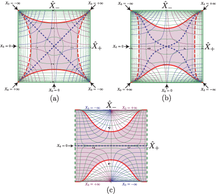
We depict the projection of minimal surfaces (6) onto the $(X_{+},X_{-})$-plane in Fig. 2(a) and the $({\hat{X}}_{+},{\hat{X}}_{-})$-plane in Fig. 3.

Firstly we consider the case $0\leq\beta<1$. Especially $\beta=0$ implies that the scattering is symmetric with respect to $s$ and $t$ (see Eqs. (3)). The causal structure on world-sheet is drawn in Fig. 3(a,b). The red solid lines are the horizons by $g_{--}=0$, i.e., Eq. (9), and the red dashed lines are the horizons by $g_{++}=0$, i.e., Eq. (10). In the red shaded regions, both of $g_{++}$ and $g_{--}$ are positive. In every figure, $g_{++}>0$ and $g_{--}<0$ in the upper and lower white regions, while $g_{++}<0$ and $g_{--}>0$ in the left and right white regions. Therefore these white regions are Lorentzian, and are separated by the (red) Euclidean region, that is, a wormhole.

Note that $g_{--}$ is negative in the upper and lower Lorentzian regions, while $g_{++}$ is negative in the left and right Lorentzian regions, and that $g_{++}$ is equal to $g_{--}$ on the blue dotted lines given by $(1+\beta)\mathop{\operator@font sh}\nolimits u_{+}=\pm(1-\beta)\mathop{\operator@font sh}\nolimits u_{-}$. It means that we can define world-sheet time as an appropriate coordinate depending on the region. Since the vertex operators can be inserted anywhere on the boundary of disk, this is completely natural. Consider a static gauge, $(\tau,\sigma)=(X_{0},Z)$. The time $\tau\,(=X_{0})$ begins at the upper-left and lower-right corners and ends up at the upper-right and lower-left ones. The thin blue (red) lines are negative (positive) constant $\tau$ lines. On the axes, $X_{\pm}=0$, $\tau$ is equal to zero. The thin green lines are constant $Z$ lines. The surface (6) implies $Z\geq 1$. $Z$ has a minimum, $Z=1$, at the origin in Fig. 1(b) and Fig. 3(a,b). $Z$ becomes infinity on the square bounding boxes, which are the AdS boundary ²² 2 The minimal surface (6) at $Z=\infty$ is laid on the AdS boundary, because simultaneously $X_{\pm}$ also goes to infinity (see Appendix A in Ref. [12])., in Fig. 3(a,b). Therefore we can recognize the thin blue and red lines as the time evolution of open strings whose endpoints are located on the AdS boundary.

The horizons (9) and (10) are at least the stationary limit curves but might be different from a horizon of usual black hole. So let us check whether there is a singularity. The Kretschmann scalar on the world-sheet (7), $R_{ijkl}R^{ijkl}$ ($i,j,k,l=\pm$), diverges on $(1-\beta)\mathop{\operator@font ch}\nolimits u_{-}-(1+\beta)\mathop{\operator@font ch}\nolimits u_{+}=\pm 2\sqrt{1+\beta^{2}}$, in other words, these curves are singularity. From Fig. 2(b), we can see that the singularity is in the interior of horizons, hence the horizons themselves are not singularity.

Next we focus on the case $\beta=1$. It is so-called the Regge limit, namely, $-s\to\infty$ with $-t$ fixed. The world-sheet metric (7) is reduced to

While $g_{++}$ is positive definite, $g_{--}$ is negative when $\mathop{\operator@font ch}\nolimits u_{+}>\sqrt{2}$, i.e., $|u_{+}|>\log(\sqrt{2}+1)$. Therefore the world-sheet horizons appear at $u_{+}=\pm\log(\sqrt{2}+1)$. The causal structure on world-sheet is depicted in Fig. 3(c), in which the red thick lines are the horizons given by $g_{--}=0$. In this case different from those in $0\leq\beta<1$, two Lorentzian regions, where $g_{++}>0$ and $g_{--}<0$, exist, and are separated by a Euclidean wormhole (red shaded).

Since a gluon is described by an open string itself, we can see two kinds of entanglement: one is the entanglement of string endpoints in a gluon, and the other is the entanglement of gluons.

In Fig. 4, $A_{L,R}$ and $B_{L,R}$ denote the endpoints of open strings describing gluons on the boundary. Since the upper-left and lower-right corners are at $X_{0}=-\infty$ and the lower-left and upper-right corners are at $X_{0}=\infty$, in the static gauge we can regard $g_{1}$ and $g_{2}$ as the incoming gluons and $g_{3}$ and $g_{4}$ as the outgoing gluons. The gluons, $g_{1}$ and $g_{2}$ at $X_{0}=t_{1}\,(<0)$ and $g_{3}$ and $g_{4}$ at $X_{0}=t_{2}\,(>0)$, can be described as the entangled states of open string endpoints, namely,

Each entanglement in the states (12) is interpreted to the fact that each open string crosses over the wormhole (see Fig. 4). Let us focus on the vicinities of the corners of (green) bounding box. The causal structure on the world-sheet which describes the entanglement of string endpoints in each gluon (e.g. $A_{R}\to B_{L}$) is similar to that of accelerating quark and antiquark in Ref. [4] .

At $X_{0}=0$ the open strings, $g_{1}$ and $g_{2}$, join and split to $g_{3}$ and $g_{4}$, in other words, the color exchange of gluonic interaction happens at the mid-point $M$ of open strings (Fig. 4). Therefore $X_{0}=0$ is the moment that the entanglement between gluons is gained. Even if the initial state of gluons is not entangled, the final state of gluons is entangled due to the interaction. From a geometric viewpoint, any paths connecting the open string gluons (e.g. $A_{R}(t_{2})B_{L}(t_{2})$ and $A_{L}(t_{2})B_{R}(t_{2})$) must cross the wormhole region (see the blue ribbon in Fig. 4).

How can we quantify entanglement of two interacting particles? In Refs. [16, 17, 18], the EE is associated with a Wilson loop by $S_{E}=(1-c\lambda\partial_{\lambda})\log\langle W\rangle$.³³ 3 The undetermined constant $c$ depends on the shape of scattering Wilson loop and is not relevant to our purpose here. (cf. $c=4/3$ for a circular Wilson loop Ref. [18].) Note that the EE itself is associated with a quantum state at a time while the Wilson loop $\langle W\rangle$ depends on the entire time dependent process. Therefore we should consider the left hand side of above mentioned equation as the change of the EE, $\Delta S_{E}$. So the gluon scattering amplitude [12] is related to the change of the EE in leading order of large $\lambda$ by

where we neglected the IR divergent pieces.

We introduce another characteristic quantity concerning about the entanglement of gluons. Let us consider the proper lengths of lines, $A_{R}(0)B_{R}(0)$ and $A_{L}(0)B_{L}(0)$, at the contacting instance $X_{0}=0$;

where we introduced the cutoff, $z_{\infty}\,(\gg 1)$, such that $(2\alpha/R^{2})z_{\infty}=(1\pm\beta)\mathop{\operator@font ch}\nolimits u_{\pm\infty}+1\mp\beta$.

$\ell_{+}$ and $\ell_{-}$ correspond to the two channels of gluon interaction. In one channel (Fig. 5(a)), the gluons $g_{1}$ and $g_{2}$ flow to $g_{3}$ and $g_{4}$ respectively. Then, the region $\Sigma$ on the boundary corresponding to the gluon $g_{1}\to g_{3}$ is drawn by the thick green line segments and the region ${\overline{\Sigma}}$ corresponding to the gluon $g_{2}\to g_{4}$ is drawn by the dotted green line segments. Since the blue line $A_{R}(0)B_{R}(0)$ in the bulk connects the boundary $\partial\Sigma$, $\ell_{+}$ is related with the entanglement of gluons in the sense of Ref. [15]. In the same way, we can consider the other channel, i.e., $g_{1}\to g_{4}$ and $g_{2}\to g_{3}$, in which $\ell_{-}$ characterizes a part of the entanglement of gluons (Fig. 5(b)).

Eq. (14) is computed as $\ell_{\pm}(\beta)=-\sqrt{6}R\log(1\pm\beta)$, where we subtracted the divergent piece, $\sqrt{6}R\log(2\alpha z_{\infty}/R^{2})$, for $z_{\infty}\to\infty$. Then the EE change (13) is also described as

where we used $R^{2}=\sqrt{4\pi\lambda}\ell_{s}^{2}$.

We comment on the Regge limit, $\beta=\pm 1$. Since the finite part of $\Delta S_{E}$ becomes minimum at $\beta=0$ and diverges at $\beta=\pm 1$, the Regge limit is the case with maximal $\Delta S_{E}$. Actually Fig. 3(c) shows that, at $\beta=1$, one of the endpoints of $g_{1}$ ($g_{2}$) always coincides with that of $g_{4}$ ($g_{3}$), and $\ell_{-}(1)$ diverges.

Can we generalize above result to more general scattering particles? We believe this is the case. To show this we give a construction by which $\Delta S_{E}$ can be identified as the scattering amplitude. First we can extend the Ryu-Takayanagi formulation of EE by allowing the subspace A and B to be the space-time regions (rather than spatial regions) whose minimal surface in AdS generates the change in the EE. In case of world-line of scattering quark-antiquark pair, it is nothing but the minimal surface calculating the Wilson lines. That is, for any two scattering particles A and B, there is an infinite line $l(t)$ connecting them at each time $t$.

As time evolves, $l(t)$ generates a two-dimensional surface in the entire space-time of boundary field theory, which we call a scattering surface (Fig. 6(a)). Then the world-lines of the two particles will divide the scattering surface into two, $\Sigma$ and ${\overline{\Sigma}}$. Considering the constantly accelerating particles whose minimal surfaces is found in Ref. [6], we can exemplify these idea. The trajectory of two particles forms a circle in Eudlideanized space-time. The minimal surface of circle is well studied, and its area is given by $-\sqrt{\lambda}/(2\pi)$ independent of the acceleration [21].

This construction shows a way to identify the scattering amplitude as a change of EE. Notice that the change of EE between initial and final states is a function of the whole scattering process. Therefore this change should be related to S-matrix.

The term, $\lambda\partial_{\lambda}\log\langle W\rangle$, in $\Delta S_{E}$ comes from the replica trick in the derivation of EE. On the other hand, in the language of scattering, that term corresponds to Bremsstralung of radiative correction. Actually in the case of accelerating quark-antiquark, $\lambda\partial_{\lambda}\log\langle W\rangle$ is proportional to the Bremsstralung function [22]. Therefore the change of EE, $\Delta S_{E}$, is related with S-matrix, which gives a scattering amplitude in principle including a radiative correction.

We studied the causal structure on the open string world-sheet of gluon scattering minimal surface in position space. On this world-sheet there exists the wormhole which separates the Lorentzian regions including the boundary. Gluons are given by the open strings. We have shown that any paths connecting such two open string gluons at any time slices pass through the wormhole. Therefore a wormhole can always be associated with the entanglement of interacting gluons. This result supports the EPR = ER conjecture.

Below, we discuss a few points which needs clarification:

• •

  One may ask why entanglement should be related to the interaction, because entanglement is property of the state not the hamiltonian. Consider scattering of two particles which are initially (at $t=-\infty$) far separated and un-entangled. We can construct the basis of in- and out- states by tensor product of free particle states. Let the initial state $|i\rangle$ to be a tensor product state $|i\rangle=|i_{1}\rangle\otimes|i_{2}\rangle$ They approach each other and interact and then go force-free region after long time $t=+\infty$. Such time evolution is given by the evolution operator $U=\exp[-iT(H_{1}+H_{2}+H_{\rm int})]$ or S-matrix:

  $$|\psi\rangle=\lim_{T\to\infty}U|i\rangle=\sum_{f}|f\rangle\langle f|S|i\rangle=\sum_{f}|f\rangle S_{fi}$$

  (16)

  which is entangled in general unless interaction $H_{\rm int}=0$ so that $U$ is factorized. So the final state of two free particles are entangled and its EE can be identified as the ‘change’ of EE of the two particle system. Our question is that how to relate the latter to the S-matrix itself, which seems to be non-trivial task in field theory setting.

• •

  If the final state involves sum over all possible quantum states, why one can consider only one world-sheet? In classical mechanics, final configuration is completely determined if initial one is given. Now in the AdS/CFT, due to the large $N$ nature, classical discussion can be made. That is, when we consider a minimal surface whose boundary is the trajectories of two scattering particles, we implicitly assumed that such classical picture is valid in describing the gluon-gluon or heavy quark-antiquark scatterings. Therefore we do not sum over trajectories and hence not sum over the world-sheets. This is the reason why we can consider the causal structure of a single world sheet of the gluon scattering instead of summing over such world-sheets. The same philosophy was implicitly assumed in the discussions of causal structure of world-sheet in recent literature. With these understanding, we observed the EE change (13), following the holographic calculations by Ref. [18]. This EE change becomes minimum at $\beta=0$ and diverges at the Regge limit $\beta=\pm 1$. The relation shows that the change of EE is a function of dynamical process, which is natural. Here it was shown by holographic argument and mostly likely it is true only in the holographic context where semi-classical nature holds. It would be interesting to see how this relation in the general quantum field theory can be written.

• •

  Another point that should be discussed further in the future is the conjecture we used: the EE of Wilson loop can be calculated by the minimal surface associated with the Wilson loop expectation value. Which was proven only simplest cases. Even providing more examples will be interesting.