An Efficient Search Strategy for Aggregation and Discretization of Attributes of Bayesian Networks Using Minimum Description Length
Abstract
Bayesian networks are convenient graphical expressions for high dimensional probability distributions representing complex relationships between a large number of random variables. They have been employed extensively in areas such as bioinformatics, artificial intelligence, diagnosis, and risk management. The recovery of the structure of a network from data is of prime importance for the purposes of modeling, analysis, and prediction. Most recovery algorithms in the literature assume either discrete of continuous but Gaussian data. For general continuous data, discretization is usually employed but often destroys the very structure one is out to recover. Friedman and Goldszmidt [11] suggest an approach based on the minimum description length principle that chooses a discretization which preserves the information in the original data set, however it is one which is difficult, if not impossible, to implement for even moderately sized networks. In this paper we provide an extremely efficient search strategy which allows one to use the Friedman and Goldszmidt discretization in practice.
AMS Subject classification: 62-09, 68P30, 62C99
1 Introduction
Bayesian networks are convenient graphical expressions for high dimensional probability distributions representing complex relationships between a large number of random variables. They have been employed extensively in areas such as bioinformatics ([4], [12], [17], [16]), artificial intelligence ([15], [13], [21]), diagnosis ([8], [18], [23]), and risk management ([7], [10], [22]) for the purposes of general modeling, prediction, and diagnosis.
A Bayesian network consists of a directed acyclic graph (DAG), in which nodes represent random variables, and a set of conditional probability distributions. For example, the graph in Figure 1 represents a network for 5 variables, , , , , and with a joint probability density which is assumed to factor as

In general, for a Bayesian network on nodes, the joint density for the corresponding random variables may be written as
| (1) |
where is used to denote the set of random variables corresponding to “parent” nodes for node . For the example in Figure 1, we have , , , , and .
Given observations of , our ultimate goal is to infer the connecting arrows for a corresponding -node graph. There are many ways to do this rather successfully for discrete data or for Gaussian data. In the case of non-Gaussian continuous data, discretization is usually employed, however care must be taken not to destroy the very structure one wishes to retrieve. Since the problem involves mapping entire intervals of values to discrete values, it is closely related to the “aggregation problem” where one reduces the number of possible values taken on by a node by mapping collections of values in already discrete data to single points. (We will think of this as a “discretization of discrete data” and will still refer to it as discretization.)
For an example of a discretization masking important attributes of the underlying network structure, consider the three node DAG show in Figure 2 where the corresponding random variables , , and each take on values in .

Consider the discretization to random variables , , and defined as if and if .
The original network structure implies that the variables represented by nodes and are conditionally independent given the value of the variable at node 1, yet it is easy to verify that we have, after discretization,
for example. Thus, there is little hope of recovering the correct network structure after this discretization with data that have been discretized in this way.
Friedman and Goldszmidt [11] suggest an approach based on the minimum description length principle that chooses a discretization which preserves the information in the original data set. However, their approach, which we describe in Section 3, requires that we compute and compare scores for every different possible discretization of the data. The number of possibilities is often prohibitively large.
In this paper we give a search strategy in which only a very small subset of minimum description length scores must be computed. Under certain simplifying assumptions, we prove that the procedure will identify the optimal score. Furthermore, in the case where there is a “correct” discretization in the sense that distributions of nodes are unchanged over entire intervals of values for children, we show that the optimal scoring network does in fact correspond to the data generating network.
2 Likelihood-Based Recovery of Bayesian Networks for Discrete Data
We will use this section to establish some notation that will be used throughout this paper and to briefly review commonly used likelihood-based methods for recovering the structure of Bayesian networks.
Consider a Bayesian network on nodes. For , let denote the random variable associated with node . We will refer to node and the associated random variable , interchangeably. Suppose that can take on values in . Let denote the set of parent node indices for node , let denote the number of parents for node , and let denote the number of possible parent configurations. For example, for the network in in Figure 1,
For , , and , define parameters
Here, “” refers to a specific set of values for the parent variables, configurations of which have been enumerated and are now indexed by .
Now, from the joint density (1), the likelihood for the entire dimensional data set may be written as
where is the total number of times in the sample that is observed to have value when its parents take on configuration . (To keep this concise expression for the likelihood, we define, for a parentless node , and .)
There are many ways to recover networks from data. Indeed, we may not even want to think in terms of “one best network” and instead use a model averaging approach or one that constructs a best network by combining best “features” (for example edges) from several networks. In this paper, we will restrict our attention to simple methods for recovering a single “best” network as measured by various standard likelihood and information criterion indices. We will assume a manageable number of networks to score. Of course, the number of possible networks increases superexponentially in the number of nodes– the results of this paper might then be applied using Monte Carlo search strategies.
- 1.
Log-Likelihood (LL)
Given -tuples of data points, we compute the log-likelihood for every possible graph. For each DAG, we have a different set of relevant parameters. Given a particular DAG, we estimate each with its maximum likelihood estimator
and then we report the log-likelihood
As we can always increase the log-likelihood by including additional parameters, we expect the greatest log-likelihoods (“most likely models”) to coincide with DAGs with a maximal number of edges. Therefore, it is important include a penalty for overparameterized models. The two most common penalized log-likelihood statistics are given by the following information criteria.
- 2.
Akaike’s Information Criterion (AIC)
Akaike’s Information Criterion (AIC) is, in its most general form, defined by
Clearly, the goal is to minimize the AIC to ensure a good fitting model in the sense of maximizing the log-likelihood while penalizing for having too many parameters.
- 3.
Bayesian Information Criterion (BIC)
The Bayesian Information Criterion (BIC) is defined by
where is, as before, the sample size. As with the AIC, the goal is to minimize the BIC.
Both the AIC and BIC have rigorous justifications, from both Bayesian and frequentist points of view. AIC was derived from information theory though it can be though of as Bayesian if one uses a clever choice of prior. On the other hand BIC, originally derived through Bayesian statistics as a measure of the Bayes factor, can also be derived as a non-Bayesian result. For more information on these widely used scoring criteria, we refer the interested reader to [1],[2], [3], and [5] (AIC), and [14] and [20] (BIC). To make some broad generalizations, AIC, it can often overfit the model in terms of number of parameters. BIC, on the other hand, tends to overpenalize, or underfit the model.That being said, we have been most successful in recovering the correct structure of simulated Bayesian networks using AIC. Incidentally, the use of Bayesian networks does not necessarily imply a Bayesian approach to modeling where parameters are considered as random variables. In this paper, we are taking the frequentist approach.
3 Minimum Description Length
Arguably, the point of statistical modeling is to find regularities in an observed data set. Discovered regularities allow the modeler to be able to describe the data more succinctly. The minimum description length (MDL) principle, introduced in 1978 by Jorma Rissanen [19], is a model selection technique that chooses, as the best model, the one that permits the shortest encoding of both the model and the observed data.
In this section, we describe how Friedman and Goldszmidt [11] define a description length that can be used for network recovery from discrete data. It is the approximate length of storage space, measured in bits, for the binary representation of the DAG (network structure), the parameters (the ) that, together with the DAG, define a Bayesian network, and the data itself. We will see, in the end, that it is simply another penalized likelihood approach.
In what follows, we repeatedly use the fact that an integer can be encoded in approximately bits. For example, the decimal value becomes, in binary, the bit number 1001. Throughout this paper, we will use to denote the base logarithm, though, in the end the base is unimportant for the comparisons we will make.
Encoding the DAG
As in Section 2, we assume that , can take on possible values, and that they are integers ranging from to . (For example, if can take on values in , we would relabel the values as , , and .)
The approximate number of bits needed to encode the number of nodes/variables , and the number of possible values taken on by each of those variables is
| (2) |
In order to completely describe the network structure, we must also include the number of parents for each node and the actual list of parents for each node. As a simplification, since the number of parents of node , which is denote by , is always less than , we can, conservatively, reserve bits to encode . Doing this for each node, we add
| (3) |
to our network description length.
For the actual list of parents, since the maximum value in the list of indices is , we will use the conservative value of bits to encode each index. For node , we must encode different indices, each using a length of bits of space. So, in total, to encode all parent lists, we will use
| (4) |
bits.
In total, we use
| (5) |
bits to encode the DAG structure.
Encoding the Parameters
The Bayesian network consists of a DAG together with a collection of parameters . Since , we only need to encode parameters for node . However, the parameters are not integer valued. In our case, for network recovery, we will actually be storing/encoding parameters that have been estimated from our -dimensional data points. Friedman and Goldszmidt [11] indicate that the “usual choice in the literature” is to use bits per parameter. Thus, we will use
| (6) |
bits to encode the estimated network parameters.
We add (5) and (6) in order to define description length for the Bayesian network. Since we are trying to infer the best connecting arrows for a graph on nodes, we presumably already know the number of nodes and would not be encoding it. Thus, we drop the term and define the network description length as
| (7) |
Encoding the Data
Consider the string of digits stored, in binary as . (The binary representations of , , and are , , and , respectively.) Without separators, the binary string can not be decoded near the end. The maybe be, in decimal, three ’s, a followed by a , or a followed by a . “Prefix codes” avoid this problem by encoding the digits with zeros and ones in a way so that no encoded digit is a prefix of any other encoded digit. Further consideration can be made to ensure the code is not only a prefix code, but one that results in the maximum compression of the data by assigning, to the original decimal digits, binary codes of lengths inversely proportional to the frequencies with which they appear in the original data.
In the context of Bayesian networks, we wish to encode the values in the -dimensional data set with code lengths that are inversely proportional to the frequencies (equivalently, estimated probabilities) with which they appear in the data. Friedman and Goldszmidt [11] use Shannon coding [6] which is not optimal in terms of compression, but which encodes each -dimensional data point using approximately bits where is the joint density for evaluated at . Thus, the entire data set, consisting of such vectors is encoded in approximately
| (8) |
bits. This is desirable from a modeling standpoint since it corresponds to the familiar log-likelihood commonly used in statistical inference.
Summing (7) and (8), we define the description length for a Bayesian network and the observed data as
| (9) |
Given discrete data and a collection of possible Bayesian networks, the network chosen by the MDL principle is the one that minimizes (9). In light of the form of , we see that this is simply a penalized log-likelihood scoring metric, similar to the AIC and BIC discussed in Section 2. We now illustrate the performance of all three for a three node network. The list of all 25 DAGs corresponding to 3 node networks can be found in Table 1 and we will refer to these DAGs as they are numbered here.
| 1 | 2 | 3 | 4 | 5 |
|---|---|---|---|---|
![[Uncaptioned image]](1404.0752v1/3nodes1.png) |
![[Uncaptioned image]](1404.0752v1/3nodes2.png) |
![[Uncaptioned image]](1404.0752v1/3nodes4.png) |
![[Uncaptioned image]](1404.0752v1/3nodes3.png) |
![[Uncaptioned image]](1404.0752v1/3nodes6.png) |
| 6 | 7 | 8 | 9 | 10 |
![[Uncaptioned image]](1404.0752v1/3nodes5.png) |
![[Uncaptioned image]](1404.0752v1/3nodes7.png) |
![[Uncaptioned image]](1404.0752v1/x1.png) |
![[Uncaptioned image]](1404.0752v1/3nodes10.png) |
![[Uncaptioned image]](1404.0752v1/3nodes12.png) |
| 11 | 12 | 13 | 14 | 15 |
![[Uncaptioned image]](1404.0752v1/3nodes9.png) |
![[Uncaptioned image]](1404.0752v1/3nodes15.png) |
![[Uncaptioned image]](1404.0752v1/3nodes17.png) |
![[Uncaptioned image]](1404.0752v1/3nodes11.png) |
![[Uncaptioned image]](1404.0752v1/3nodes13.png) |
| 16 | 17 | 18 | 19 | 20 |
![[Uncaptioned image]](1404.0752v1/3nodes14.png) |
![[Uncaptioned image]](1404.0752v1/3nodes18.png) |
![[Uncaptioned image]](1404.0752v1/3nodes19.png) |
![[Uncaptioned image]](1404.0752v1/3nodes16.png) |
![[Uncaptioned image]](1404.0752v1/3nodes20.png) |
| 21 | 22 | 23 | 24 | 25 |
![[Uncaptioned image]](1404.0752v1/3nodes21.png) |
![[Uncaptioned image]](1404.0752v1/3nodes22.png) |
![[Uncaptioned image]](1404.0752v1/3nodes23.png) |
![[Uncaptioned image]](1404.0752v1/3nodes24.png) |
![[Uncaptioned image]](1404.0752v1/3nodes25.png) |
We fixed arbitrary parameters for DAG 8 in Table 1 and simulated values of . (Each was assumed to take on values in .)
Results are shown in Table 2 along with the previously computed values of AIC and BIC. The AIC, BIC, and MDL scores all recovered the correct network ‘‘up to Markov equivalence’’.†† A set of DAGs with the same set of edges are said to be Markov equivalent if they share the same set of conditional independence relations among variables. Recovering the specific graph within a Markov equivalence class (a causality problem) requires experimental as opposed to simply observed data and is not the subject of this paper.
| Graph | AIC | BIC | MDL |
|---|---|---|---|
| Number | |||
| 1 | 1040886.085 | 1041057.317 | 520443.714 |
| 2 | 1001501.922 | 1001958.543 | 500885.425 |
| 3 | 1001501.961 | 1001958.543 | 500885.425 |
| 4 | 991255.256 | 991711.879 | 495762.093 |
| 5 | 991255.259 | 991711.879 | 495762.093 |
| 6 | 1036182.434 | 1036639.054 | 518225.681 |
| 7 | 1036182.434 | 1036639.054 | 518225.681 |
| \CT@next | |||
| 8 | 951871.096 | 952613.104 | 476213.804 |
| 9 | 951871.096 | 952613.104 | 476213.804 |
| 10 | 951871.096 | 952613.104 | 476213.804 |
| 11 | 996798.271 | 997540.279 | 498677.392 |
| 12 | 996798.271 | 997540.279 | 498677.392 |
| 13 | 996798.271 | 997540.279 | 498677.392 |
| 14 | 991435.745 | 936604.692 | 496536.904 |
| 15 | 986551.608 | 987293.616 | 493554.060 |
| 16 | 986551.608 | 987293.616 | 493554.060 |
| 17 | 986551.608 | 987293.616 | 493554.060 |
| 18 | 956755.233 | 958924.180 | 479196.648 |
| 19 | 952051.582 | 954505.917 | 476988.615 |
| 20 | 952051.582 | 954505.917 | 476988.615 |
| 21 | 952051.582 | 954505.917 | 476988.615 |
| 22 | 952051.582 | 954505.917 | 476988.615 |
| 23 | 952051.582 | 954505.917 | 476988.615 |
| 24 | 952051.582 | 954505.917 | 476988.615 |
| 25 | 952051.582 | 954505.917 | 476988.615 |
4 Minimum Description Length for Discretization
A discretization of data for the random variable , represented by node , is a mapping from the range of values in the data set to the set for some . It can be described by ordering the distinct values observed for and inserting up to “thresholds”. For example
| (10) |
In this paper, we will assume that only node needs to be discretized and that the remaining nodes are discrete or have already been discretized. We refer the reader to Friedman and Goldszmidt [11] for a discussion of multiple node discretization which essentially involves fixing discretizations for all but one node, discretizing that node, and repeating the process by cycling through all nodes repeatedly.
As before, we assume that we have observations of the -dimensional . Let be the number of distinct values taken on by in the data set. Note that , with equality possible only for truly continuous data. Define as the discretized version of . To discretize to values, we need to choose thresholds to put in spaces between ordered values. There are threshold configurations to consider. Since we will not know in advance how many values we should have in the discretized data set, we need to consider everything from , which corresponds to mapping all values for in the data set to the single value of 1, to , which corresponds to no discretization at all. In total, there are
discretizations to consider.
Friedman and Goldszmidt [11] define a description length score for a network with discretized into a particular configuration of thresholds using essentially four terms. These terms include and , previously described in (7) and (8), computed now after discretization– we will call these terms and . Also included are terms that encode the index denoting a particular discretization policy and description length for information needed to recover the original data from the discretized data.
Encoding the Discretization Policy
For fixed and , there are different possible configurations for thresholds. Assume we have labeled them from to . Storing the index for a particular policy will take at most bits. Friedman and Goldszmidt use a conservative upper bound based on the inequality
where
and conservatively reserve
| (11) |
to encode the discretization policy. (In practice, we define .)
Encoding Recovery of Original Data
Consider again the example of 9 () distinct values for given by (10) from a data set with values. Every time we assign a discretized value to an original value, we should store the original value for recovery. Instead, however, we will store the Shannon binary code for the original value using estimated conditional probabilities based on the entire data set. For example, the value might appear in the entire data set one-fourth of the time. That is, . Among the instances of , , and , it might appear half of the time. That is, . Given a discretized value of , we will encode the original value, , using approximately bits. In total, for recovering original data from discretized data, we add
| (12) |
to the description length.
In summary, Friedman and Goldszmidt [11] define the description length discretization score as
| (13) |
Given a data set and a particular network structure, one scores various discretization mappings for and chooses the discretization that minimizes (13). For a given network, the score in (13) will change over discretizations only in terms directly linked to the th node. Thus, as Friedman and Goldszmidt point out, we only need to consider the “local description length score” defined, by picking out relevant terms, as
| (14) |
Here, is a the set of parents for node , denoted with an asterisk since it includes the discretized , and,
| (15) |
is the estimated mutual information between random vectors and . ( is defined to be zero.)
5 Minimizing the Local Description Length Score
Computation of a single value of (14), which is based on network structure through the information terms, can be quite time consuming. For even moderately sized , computation of (14) repeatedly to check all discretization policies can be prohibitive, and when multiple/all nodes need to be discretized (a procedure that involves several passes through each node as discussed in [11]), computation of (14) becomes almost impossible. Friedman and Goldszmidt [11] give some further computational simplifications and suggest a greedy search routine.
The purpose of this paper is to provide an alternative efficient search strategy for the smallest score. We assert that, for a single node discretization, one need only check values of as opposed to . Multiple continuous nodes can then be cycled for discretization just as Friedman and Goldszmidt have suggested.
For notational simplicity, we assume, for the remainder of this paper, that the node to be discretized is labeled as node . Also, as we are comparing values of for various discretizations of , we will drop all asterisk superscript notation, as it is understood that we are considering discretized values.
Single Threshold Top-Down Search Strategy
Let be (14) with all thresholds in place. For , let be (14) with all thresholds except for the th threshold.
In order to minimize over all discretization policies for , make comparisons of with for . If , remove the th threshold.
We first consider the effectiveness of this search strategy in the very ideal situation where we augment given discrete data by introducing superfluous values for node 1 in a larger discrete set. For example, we might replace values of in the original data set with values in with some arbitrary probabilities, whereupon we hope that our search strategy will minimize and that the configuration of thresholds that does such will correctly map values in back to the original value of . We will prove, in this case, that the “single threshold top-down” search strategy will find the discretization policy that minimizes among all discretizations for a large enough sample size .
Indeed, , , , and are constant, and . Note that
| (16) |
will be constant over any discretization policy for with a fixed number of thresholds. In particular, when comparing all possible single threshold removals, starting with any fixed number of thresholds, we can restrict our attention to maximizing
| (17) |
In the next Section, we consider what our search strategy does to (17) in the absence of (16) in an ideal situation where there is a “correct” discretization. We will see that it maximizes (17) and that it does so while leaving a minimal number of thresholds. In Section 5.2, we will consider (16) and conclude that we are indeed minimizing . We will also see that it finds the correct discretization.
5.1 A Closer look at Information Terms in an Ideal Situation
As the notation to follow gets a bit cumbersome in the general case, we illustrate the proof of most claims in this Section and the next with a concrete example. Consider a two-node network where node is a parent to node , and assume that that both nodes take on values in . From data points, we can produce estimates
for .
In general, for this two node network, we would assume that node 1 takes on values in , node 2 takes on values in , and one would work with the estimates , , and for and .
We now “explode” the data for our specific example at node into values in by replacing instances of with values in with probabilities and , respectively, replacing original instances of with values in with probabilities , , and , respectively, and replacing original instances of with the value . Thus, in our “exploded data set”, node is taking on values in with probabilities denoted as for , where, for example, and . Joint probabilities for and are denoted by where we have, for example,
In the more general case, we could “explode” the data at node more generally by replacing instances of with values in some probabilities , summing to 1, replacing original instances of with values in with respective probabilities , summing to 1, and so forth.
By “exploding” the data at node one, we have introduced superfluous values for in terms of probabilities for . For example, for all . Any proper discretization process should aggregate the values and for back into one value. Here, is used to denote the probability . Similarly, may be denoted as .
For this two-node network, (17) is simply , which we will denote by . Define this estimated information as
| (18) |
where
| (19) |
and the sums run over and .
Define the corresponding information and information terms using in place of with sums running over and .
It is easy to verify information term relationships such as
and consequently that
That is, we did not change the information between and by exploding the data at .
We now show that our single threshold top-down search strategy will correctly recover the original values for . We call this the “correct discretization”, denoted as , which means that we will remove three thresholds from the “full discretization”, denoted as , and that the values and will map back to , the values in will map back to , and the value , will map back to . We will assume that the original values in are all distinct in the sense that for some , for some , and for some , so that they should not be aggregated further.
Removing a Threshold: The Impact on Information
Starting with the exploded data, with values for represented as , we consider the information term after removing the threshold between the values and for some . Note that removal of this th threshold will leave all values below the threshold unchanged, while all values above will be decreased by 1. For example, if we remove the third threshold, we denote the new configuration as , but it represents a mapping
Define, for and , the joint and marginal probabilities for and after the th threshold is removed as , , and . We have, for , the relationships
and
Defining and analogous to (18) and (19), using , we have, for ,
The inequality is is due to the log-sum inequality,
which holds for any nonnegative and . The log-sum inequality can be shown to be an equality if and only if the are equal for all . Thus, we have that
| (20) |
for , with equality if and only if
This happens if and only if
| (21) |
for , which is precisely when the values and in the exploded version of should be aggregated or discretized into one value. If we do not have (21), aggregating the values will result in a loss of information.
Note that denotes the value of the information between and with the th threshold in the explosion for removed. In our example,
and
Thus, we have (21), when , and consequently
On the other hand, considering the second threshold removal from the full discretization , similar calculations show that
which is not, in general, equal to
so we have the strict inequality and therefore
In all, we can show in this way that
| (22) |
So, our search strategy will produce the correct discretization . The question remains though as to whether this is actually the discretization that minimizes . Due to (20), we will always have . In fact, due to the log-sum inequality, any removal of a threshold from any configuration with any number of thresholds can never increase information. Thus, the full discretization will always have maximal information. From (22), we see that the discretizations , , and have the same, and thus also maximal, information. Note that each of these three configurations corresponds to a different explosion of the original data. This is illustrated for in Figure 3.
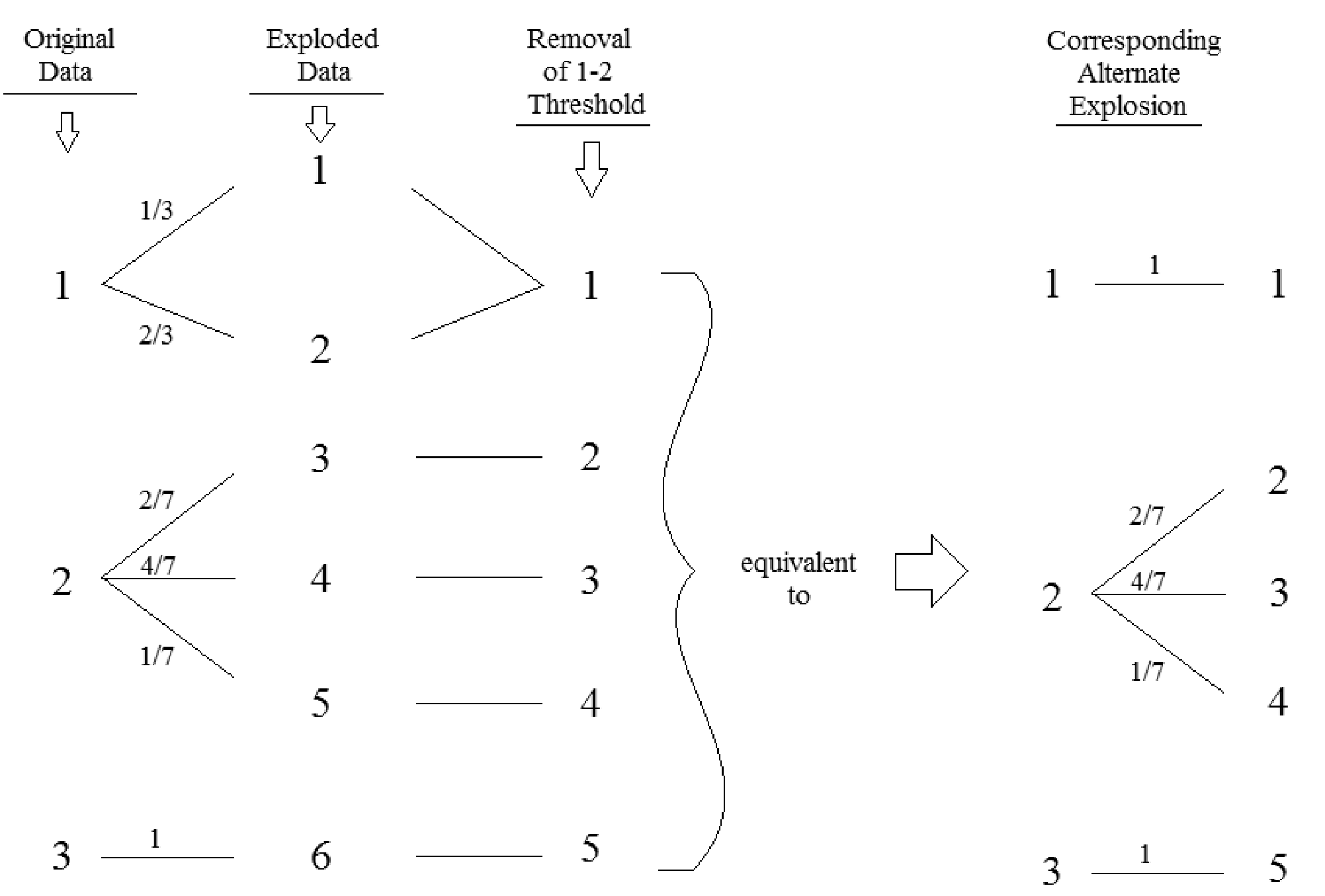
Thus, by the same information arguments above, “correct removal” (removal of one of the superfluous thresholds) of a threshold from will result in another configuration with the same maximal information. Since this is true starting with any one of the three correct single threshold removal configurations, we see that we can remove two of the superfluous thresholds from the full explosion and still maintain the maximal information. Continuing this argument, we can remove all superfluous thresholds from the full discretization and the resulting configurations of thresholds, which in this example is , will have the maximal information.
5.2 A Closer look at the Leading Terms in
For a general DAG, the leading terms in , given in (16) can be rewritten as
for some where if and only if node is not connected to any other nodes.
The second and third terms here are clearly increasing in . The first term, as a function of , is symmetric about , increasing to the left of this value and decreasing to the right. However, since
we can, when choose (the sample size) large enough to ensure that is increasing in . In this case, this first part of acts as a penalty term and is minimized by choosing the discretization that maximizes the information terms with the minimum number of thresholds. By design, the single threshold top-down search strategy will do exactly this. Thus, when employing the strategy for large samples, we can ignore these leading terms.
5.3 More Complicated Networks
The observations in Section 5.2 were not dependent on the specific network, however, our analysis of the information terms was for a two-node network where was a parent to . Since , our search strategy will also find the “optimal discretization” for , i.e. the one that that maximizes (17) with a minimum number of thresholds, for the two-node network where is a child of .
We will now check that the strategy will find the optimal discretization for for general networks. To this end, we begin by independently considering the two types of terms in (17).
- •
Since replacing with a vector of random variables has no effect on any of the computations in Section 5.1, we see that our search strategy will find the discretization for that maximizes with a minimum number of thresholds.
- •
where
Suppose, for ease of exposition, that and, that all nodes originally take values in , and that has been exploded to take values in just as in, and using the same probabilities as, Section 5.1. If consists only of , we have already seen that our search strategy will maximize the information term with a minimum number of thresholds. Assuming now that consists of and some vector whose components are the other parents of , we have
where
Here, , , and . Using to denote probabilities after the explosion of , it is easy to see expected relationships such as
Therefore, we can verify, for example, that , and that the overall information terms and are equal. We can also verify, using the log-sum inequality, that after removal of the th threshold we have
with equality if and only if
(23) Summing over all appropriate values for indices, we get that , the information term between and its parents after removal of the th threshold for , is less than or equal to , with equality if and only if (23) holds for all and . When , for example, both sides of (23) are equal to , indicating that the first threshold should be removed. When , the left side is equal to and the right side is equal to , so we do not have (23) and hence a decrease in information. Thus, we would not remove the second threshold.
, the information with all thresholds in place, is the maximal information among all possible discretizations. If we remove each threshold that leaves the information unchanged, we will still have the maximal information with a minimum number of thresholds. Thus, the top-down search strategy will give the optimal discretization.
Considering all terms in (17) independently may result in different discretizations. For example, consider graph 8 from Table 1. In this case, (17) becomes . If for all but for some , removing the threshold between and for the discretization of would leave the information between and unchanged but would decrease he information between and . However, as both information terms, and hence their sum, are maximized with the full discretization for , the top down-search strategy will not allow us to remove the threshold between and . That is, it will only remove thresholds between values of that are indistinguishable in terms of the conditional distributions involving all nodes to connected to .
6 Conclusions
We have seen, in the case of ideal “exploded” data where there is a “correct” discretization, that the minimum description length scoring mechanism of Friedman and Goldszmidt will in fact recover the discretization. Just as importantly, we have seen that we can find it from among possibilities by making only comparisons.
In the case of discrete data where superfluous values were not manufactured, for example the two-node network where is a parent to that originally takes values in and , respectively, we should aggregate and for node into a single value if for all . From the data, we will only get to see that . Even with a large sample size, because of the approximation, we would still see some decrease in overall information when correctly removing the threshold, so it remains to determine when such a decrease is significant. We have much empirical evidence that we will still be able to recover the correct discretization by comparing for only single threshold removals to for the full discretization. As an example, we simulated values for and in the two-node network by simulating in directly (as opposed to first simulating them in and then exploding the data). We chose parameters such that and for all . In Table 3, we show the full discretization score, all single threshold removal scores, and the true discretization score. The two incorrect threshold removals (between 1 and 2 and between 5 and 6) stand out as having different scores than the rest. The quantification of this difference is still ongoing work.
| Discretization | DL local |
|---|---|
| -29841.52 | |
| -29870.53 | |
| -24456.07 | |
| -29866.02 | |
| -29896.74 | |
| -24585.90 | |
| -29929.17 |
Computation of the score requires that one have a graph under consideration. Indeed, all or our arguments in this paper have been made using the correct generating graph. In practice, it seems that we can still recover the correct discretization using any graph as long as the node to be discretized is connected to at least one other node which, incidentally, is precisely when we can ignore the leading terms in as discussed in Section 5.2. We recommend running the search for the discretization that minimized on several networks. Fortunately, our proposed fast search strategy makes this feasible.
The case of truly continuous data is still problematic. For the approach of this paper, it is incorrect to use estimates of densities and information terms for continuous random variables, as the procedures discussed all involve comparisons of scores computed after proposed discretizations. Consider again the two node network where is a parent of and node is the one to be discretized. (Recall that the MDL discretization process is for one node at a time. It is assumed that other nodes have already been discretized and that they will be “re-discretized” pending discretization of the current node in a cyclic fashion.) Relabel the distinct values observed for as through . We should aggregate and for node into a single value if for all , however approximations of such probabilities will can only be or ! Perhaps then, a bottom-up approach to minimizing would be better though we have not, as yet, had great success with simulated results. This too is ongoing work.
References
- [1] H. Akaike. Information theory and an extension of the maximum likelihood principle. In B.N. Petrov and F. Csaki, editors, Second international symposium on information theory, pages 267–281. Budapest: Academiai Kiado, 1973.
- [2] H. Akaike. A new look at the statistical model identification. IEEE Transactions on Automatic Control, 19(6):716–723, 1974.
- [3] H. Akaike. Likelihood of a model and information criteria. Journal of Econometrics, 16:3–14, 1981.
- [4] J. Bockhorst, M. Craven, D. Page, J. Shavlik, and J. Glasner. A Bayesian network approach to operon prediction. Bioinformatics, 19:1227–1235, 2003.
- [5] H. Bozdogan. Akaike’s information criterion and recent developments in information complexity. Journal of Mathematical Psychology, 44:62–91, 2000.
- [6] T.M. Cover and J.A. Thomas. Elements of Information Theory. John Wiley & Sons, Hoboken, New Jersey, 2006.
- [7] R.G. Cowell, R.J. Verall, and Y.K. Yoon. Modeling operational risk with Bayesian networks. Journal of Risk and Insurance, 74:795–827, 2007.
- [8] D.I. Curiac, G. Vasile, O. Banias, C Volosencu, , and A. Albu. Bayesian network model for diagnosis of psychiatric diseases. In Proceedings of the ITI 2009 31st International Conference on Information Technology Interfaces, pages 61–66. 2009.
- [9] C.O. Daub, R. Steur, J. Selbig, and S. Kloska. Estimating mutual information using B-spline functions – an improved similarity measure for analysing gene expression data. BMC Bioinformatics, 5:118:1471–2105, 2004.
- [10] N. Fenton and M. Neil. Risk Assessment and Decision Analysis with Bayesian Networks. CRC Press, Taylor & Francis Group, Boca Raton, FL, 2013.
- [11] N. Friedman and M. Goldszmidt. Discretizing continuous attributes while learning Bayesian networks. In Proceedings of ICML-1996, pages 157–165.
- [12] N. Friedman, M. Linial, I. Nachman, and D. Pe‘er. Using Bayesian networks to analyze expression data. Journal of Computational Biology, 7:601–620, 2000.
- [13] T.L. Griffiths, C. Kemp, and J.B. Tenenbaum. Bayesian models of cognition. In R. Son, editor, Cambridge Handbook of Computational Cognitive Modeling, pages 59–100. Cambridge University Press, 2008.
- [14] R.L. Kashvap. A Bayesian comparison of different classes of dynamic models using empirical data. IEEE Transactions on Automatic Control, 22(5):715–727, 1977.
- [15] K. Korb and A. Nicholson. Bayesian Artificial Intelligence. Chapman and Hall/CRC, Boca Raton, FL, 2003.
- [16] P. Larrañaga, B. Calvo, R. Santana, C. Bielza, J. Galdiano, I. Inza, J. Lozano, G.Santafè R. Armañanzas, A. Pèrez, and V. Robles. Machine learning in bioinformatics. Briefings in Bioinformatics, 7(1):86–112, 2005.
- [17] R. Mourad, C. Sinoquet, and P. Leray. A hierarchical bayesian network approach for linkage disequilibrium modeling and data-dimensionality reduction prior to genome-wide association studies. BMC Bioinformatics, 12(1):16, 2011.
- [18] A. Onisko, M.J. Druzdzel, and H. Wasyluk. A Bayesian network model for diagnosis of liver disorders. Proceedings of the Eleventh Conferenceon Biocybernetics and Biomedical Engineering, 2:842–846, 1999.
- [19] J. Rissanen. Modeling by shortest data description. Automatica, 14(5):465–658, 1978.
- [20] G. Schwartz. Estimating the dimension of a model. The Annals of Statistics, 5(2):461–464, 1978.
- [21] J.B. Tenenbaum, T.L. Griffiths, and C. Kemp. Theory-based Bayesian models of inductive learning and reasoning. Trends in Cognitive Sciences, 10(7):309–318, 2006.
- [22] P. Weber, G. Medina-Oliva, C. Simon, and B. Iung. Overview on Bayesian networks applications for dependability, risk analysis and maintenance areas. Engineering Applications of Artificial Intelligence, 25(4):671–682, 2012.
- [23] Y. Xiang, B. Pant, A. Eisen, M.P. Beddoes, and D. Pool. Multiply sectioned Bayesian networks for neuromuscular diagnosis. Artificial Intelligence in Medicine, 5:293–314, 1993.