Fluctuation and dissipation in de Sitter space

In 1827, Robert Brown noticed that pollen particles suspended in a fluid undergo an erratic motion [96], which is known nowadays as Brownian motion. Mathematically, this process is described in terms of a Langevin equation which takes into account the random kicks received by the constituents of the fluid [97, 98, 99]. In its simplest version, the Langevin equation describing the motion of a massive particle in one spatial dimension can be written as

$$\dot{p}(t)=-\gamma_{0}\,p(t)+R(t)\ ,$$

(11)

where $p(t)=m\,v(t)$ is the momentum of the particle, $m$ its mass and $v(t)=\dot{x}(t)$ its velocity. In equation (11), we assumed that the particle is much heavier than the fluid constituents and, therefore, its motion is non-relativisitic. The terms appearing in the right-hand side of this equation are the friction and random forces, respectively, and the constant $\gamma_{0}$ is known as the friction coefficient. In this description, the particle loses energy to the thermal bath because of the friction term and, at the same time, receives random kicks as prescribed by the random force.

As a first approximation, we can model the random force as white noise, with the following statistical averages:

$$\langle R(t)\rangle=0,\qquad\langle R(t)R(t^{\prime})\rangle=\kappa_{0}\delta(t-t^{\prime})\ ,$$

(12)

where the constant $\kappa_{0}$ measures the strength of the random force. Due to the fluctuation-dissipation theorem, this constant is related to the friction coefficient through

$\displaystyle\gamma_{0}$

$\displaystyle={\kappa_{0}\over 2\,m\,T}\ .$

(13)

This results from the fact that friction and random forces originate from the same mechanism at the microscopic level, i.e. collisions with the particles of the thermal bath.

One can explore the physical consequences of equation (11). One important result concerns to the time evolution of the mean squared displacement [97]:

$\displaystyle{\langle{s(t)^{2}}\rangle}\equiv{\langle{[x(t)-x(0)]^{2}}\rangle}={2\,T\over\gamma_{0}^{2}\,m}\,\left(\gamma_{0}\,t-1+e^{-\gamma_{0}\,t}\right)\approx\begin{cases}\displaystyle{T\over m}\,t^{2}&\displaystyle\left(\gamma_{0}\,t\ll 1\right)\ ,\\[12.91663pt] \displaystyle\frac{2\,T}{\gamma_{0}\,m}\,t&\displaystyle\left(\gamma_{0}\,t\gg 1\right)\ .\end{cases}$

(14)

For $t\ll\gamma_{0}^{-1}$, the motion is inertial ($s\sim v\,t$) with a velocity given by the equipartition of energy, $m\,v^{2}\sim T$. On the other hand, for $t\gg\gamma_{0}^{-1}$, the particle behaves as in a random walk ($s\sim\sqrt{D\,t}$). This crossover between the ballistic and diffusive regimes takes place in a time scale of order

$$t_{\text{relax}}\sim\gamma_{0}^{-1},$$

(15)

in which the Brownian particle loses memory of its initial conditions and thermalizes.

In $n>1$ spatial dimensions we can write down an equation equivalent to (11), where $p$ and $R$ are replaced by $n$-component vectors, and $\gamma_{0}$ and $\kappa_{0}$ become rank-two tensors, $\Gamma$ and $\mathcal{K}$ respectively. If the plasma is isotropic, i.e. if $\Gamma_{ij}=\gamma_{0}\,\delta_{ij}$ and $\mathcal{K}_{ij}=\kappa_{0}\,\delta_{ij}$ for $i,j=1,\dots,n$, then the equations of motion along the different directions decouple. In such case, the displacement squared (14) at late times goes instead as ${\langle{s(t)^{2}}\rangle}\approx 2nTt/\gamma_{0}m$. The fluctuation-dissipation theorem (13), on the other hand, is unaffected by the number of dimensions.

Now let us focus on the de Sitter space. In this case, there are at least two new effects that cannot be accounted for in the usual Langevin equation (11). The first one is that, from the point of view of a static observer (sitting at $r=0$), any particle away from the origin will feel a gravitational force acting upon it. For non-relativistic motion this force is simply given by

$$\vec{F}_{\text{grav}}=-m\vec{\nabla}\Phi,$$

(16)

where $\Phi$ denotes the Newtonian gravitational potential. This can be directly read off from the 00-component of the metric tensor, which in the weak field limit can be written as $g_{00}=-(1+2\Phi)$.⁹⁹ 9 See for instance [100]. In particular, for the de Sitter metric (8) we obtain

$$\Phi(r)=-\frac{1}{2}H^{2}r^{2}\ ,$$

(17)

i.e. a quadratic inverted potential. This means that any massive particle away from the origin will feel a repulsive force, $\vec{F}_{\text{dS}}=mH^{2}r\hat{r}$, that pushes it towards the horizon.

The second effect is the redshift of energies induced by the gravitational field. More specifically, the way a static observer has access to other points of spacetime and in particular, to our Brownian particle, is by collecting ‘photons’ or ’gravitons’ that are radiated away (or reflected) by the particle itself. Due to the gravitational redshift, the wavelength or energy observed at the center is actually lower than the energy of the particle when it was created. This is ultimately a result of the gravitational time dilation— the fact that the rate at which time passes depends on a local clock at each point of spacetime.

These two effects, the gravitational force and the redshift of energies, are correctly encoded in the classical equation of motion for a test particle— see appendix A for details. In particular, radial time-like geodesics in de Sitter space satisfy

$$\ddot{r}(t)=H^{2}r(t)\left(1-H^{2}r(t)^{2}\right)-\frac{3H^{2}r(t)\dot{r}(t)^{2}}{1-H^{2}r(t)^{2}}\ ,$$

(18)

where $\dot{\,}\equiv d/dt$. In addition to this, the particle can interact quantum mechanically with the bath of Hawking radiation emitted by the cosmological horizon, effect that is not encoded in (18). Phenomenologically, this could be taken into account by putting this particle at finite temperature in a similar way to equation (11). However, given the structure of (18), one can see that this would lead to a nonlinear Langevin equation. The problem becomes analytically tractable by focusing on the regime $\dot{r}\ll 1$ and $Hr\ll 1$. In this case, (18) leads to

$$\ddot{r}(t)=H^{2}r(t)\ ,$$

(19)

which is linear in $r(t)$. Notice that this is exactly the equation of motion of a particle in an inverted quadratic potential of the form (17), and is valid for non-relativistic motion and small deviations from the origin. On the other hand, in de Sitter space the physics is isotropic as seen by a static observer. Therefore, we can focus on the case of Brownian motion along one of the spatial dimensions ($n=1$), say $x$. In the presence of a thermal bath, one could postulate the following generalization of the Langevin equation (11):¹⁰¹⁰ 10 In the non-relativistic limit $p(t)=m\dot{x}(t)$.

$$\dot{p}(t)=-\gamma_{0}\,p(t)+F_{\text{grav}}(t)+R(t)\ ,$$

(20)

with $F_{\text{grav}}(t)=mH^{2}x(t)$ and $R(t)$ satisfying (12). Equation (20) should capture the main properties of the physics, but it fails to give a physically consistent picture for sufficiently short times $t$, in which the particle suffers only a few or no impacts. It is a general feature of any dynamical system that the dynamical coherence becomes predominant in short time scales, or at high frequencies. In this regime, equation (20) is not realistic enough for the following reasons: first, it assumes that the friction acts instantaneously and, second, that the random force is uncorrelated at different times. In a general QFT, the interactions between the Brownian particle and the medium are nonlinear and these two assumptions will no longer hold; the friction will depend on the trajectory of the particle, and random forces at different times will be generally correlated. In de Sitter space, we expect these two effects to receive further corrections coming from the curvature of spacetime. In particular, it is known that for orbits of the killing field $\xi$ away from the origin, the temperature will experience a gravitational blueshift according to [1, 2]

$$T(r)={k_{h}\over 2\pi\sqrt{-\xi\cdot\xi}}=\frac{T_{\text{dS}}}{\sqrt{1-H^{2}r^{2}}}=T_{\text{dS}}\left(1+\frac{1}{2}H^{2}r^{2}+\mathcal{O}(H^{4}r^{4})\right)~.$$

(21)

This means that the Brownian particle will have to interact with more and more Hawking quanta as it moves away from the origin. This new feature in de Sitter space is expected to modify substantially the physics at late times, or equivalently, low frequencies. Nevertheless, we will assume that the combination of all these effects can be taken into account via a generalized Langevin equation [101, 102],

$$\displaystyle\dot{p}(t)=-\int_{-\infty}^{t}dt^{\prime}\,\gamma(t-t^{\prime})\,p(t^{\prime})-k\,x(t)+R(t)+F_{\text{ext}}(t)\,,\qquad k\equiv-m\,H^{2}\,,$$

(22)

where the friction is now nonlocal and depends on the entire history of the motion through the memory kernel $\gamma(t)$. The random force is also generalized to

$\displaystyle{\langle{R(t)}\rangle}=0,\qquad{\langle{R(t)R(t^{\prime})}\rangle}=\kappa(t-t^{\prime}),$

(23)

for some function $\kappa(t)$. Moreover, we have included an extra term $F_{\text{ext}}(t)$ which is an external force that can be applied to the particle.

We believe that some of these new effects in de Sitter space can be inferred from the theory of Brownian motion in an inhomogeneous medium, a topic that has been studied extensively in the condensed matter literature [103, 104, 105, 106, 107, 108, 109, 110, 111] and is known to have some peculiar properties. In the presence of a potential field, for instance, a hot zone drives the diffusing particles up the potential slope. This is the so-called blow-torch theorem [111]. Diffusion properties in inhomogeneous media have no universal generalization, and the behavior depends on the precise physical mechanism that causes the diffusion [109]. In general, the late time behaviour of the displacement squared is modified according to

$${\langle{s(t)^{2}}\rangle}\sim D\,t^{\alpha}\,,\qquad\gamma_{0}\,t\gg 1\ ,$$

(24)

where $D$ is the diffusion constant. If $\alpha>1$, the phenomenon is called super-diffusion. The case $0\leq\alpha<1$, on the other hand, is known as sub-diffusion. Recently, this kind of anomalous behavior was observed experimentally in several systems including ultra-cold atoms [112], and various biological systems [113, 114, 115].

One way to analyze the diffusion properties of an inhomogeneous system is by considering a phenomenological equation that takes into account an effective force due to the gradient of temperature [110]

$$F_{\text{eff}}=-\frac{d\Phi}{dx}+a(T)\frac{dT}{dx}\ ,$$

(25)

where $a(T)$ is a function that depends on the microscopic model of the host medium. If the force is confining (i.e. if it diverges for $x\to\infty$) equipartition does not generally hold and the stationary solution of the diffusion equation will not be a Maxwell-Boltzmann distribution. In such cases the particle is expected to undergo sub-diffusion $0\leq\alpha<1$. We argue that Brownian motion in de Sitter space corresponds to the critically damped case $\alpha=0$ for one simple reason: the classical equation of motion for a radial geodesic (18) predicts itself that $r(t)\to 1/H$ as $t\to\infty$ and the inclusion of temperature cannot make it better. We conclude that, in this case, it is reasonable to expect that ${\langle{s(t)^{2}}\rangle}\to D$ as $t\to\infty$, where $D<1/H^{2}$, i.e. that there is an equilibrium point at which the gravitational repulsion balances with the effects of the gradient of temperature. We will corroborate this by explicit computation in section 4.2. In addition, we will show in appendix D that the distribution of velocities does not follow a Maxwell-Boltzmann distribution.

Before closing this section, let us analyze some properties of the generalized Langevin equation (22). In frequency domain, this equation can be written as¹¹¹¹ 11 Causality imposes that $\gamma(t)=0$ for $t<0$ so $\gamma[\omega]$ in this expression denotes the Fourier-Laplace transform, $$\gamma[\omega]=\int_{0}^{\infty}dt\,\gamma(t)\,e^{i\omega t},$$ while $p(\omega)$, $R(\omega)$, and $F_{\text{ext}}(\omega)$ are Fourier transforms, e.g., $$p(\omega)=\int_{-\infty}^{\infty}dt\,p(t)\,e^{i\omega t}.$$

$$p(\omega)=\frac{R(\omega)+F_{\text{ext}}(\omega)}{\gamma[\omega]-i\omega+i\frac{k}{\omega m}}\,.$$

(26)

Taking the statistical average of the same, we get

$$\langle p(\omega)\rangle=\mu{(\omega)}F_{\text{ext}}{(\omega)}\,,$$

(27)

where the quantity

$$\mu(\omega)=\frac{1}{\gamma[\omega]-i\omega+i\frac{k}{\omega m}}$$

(28)

is known as the admittance. Thus, we can determine the admittance $\mu(\omega)$, and hence $\gamma[\omega]$, by applying an external force $F_{\text{ext}}{(\omega)}$ to the Brownian particle and then measuring the response $\left\langle p(\omega)\right\rangle$. In particular, if we take

$$F_{\text{ext}}(t)=F_{0}e^{-i\omega t}\,,$$

(29)

then $\left\langle p(t)\right\rangle$ evaluates to

$$\left\langle p(t)\right\rangle=\mu(\omega)F_{0}e^{-i\omega t}=\mu(\omega)F_{\text{ext}}(t)\,.$$

(30)

From the admittance $\mu(\omega)$ we can extract

$$\gamma[\omega]=\frac{1}{\mu{(\omega)}}+i\omega-i\frac{k}{\omega m}\,,$$

(31)

and, in the low frequency limit,

$$\gamma_{0}=\lim_{\omega\rightarrow 0}\mathbf{Re}{\left(\frac{1}{\mu{(\omega)}}\right)}\,,\qquad\frac{k}{m}=\lim_{\omega\rightarrow 0}\mathbf{Im}{\left(\frac{\omega}{\mu{(\omega)}}\right)}\,.$$

(32)

Finally, when the external force is set to zero in (26), it follows that

$$p(\omega)={R(\omega)\over\gamma[\omega]-i\omega+i\frac{k}{\omega m}}=\mu(\omega)R(\omega),$$

(33)

and then, the power spectrum reads¹²¹² 12 For a quantity ${\mathcal{O}}$, the power spectrum $I_{\mathcal{O}}(\omega)$ is defined as $$I_{\mathcal{O}}(\omega)\equiv\int_{-\infty}^{\infty}dt\left\langle{\mathcal{O}}(t){\mathcal{O}}(0)\right\rangle e^{i\omega t},$$ and it is related to the two-point function through the Wiener-Khintchine theorem $$\left\langle{\mathcal{O}}(\omega){\mathcal{O}}(\omega^{\prime})\right\rangle=2\pi\delta(\omega+\omega^{\prime})I_{\mathcal{O}}(\omega).$$

$$I_{p}(\omega)=\left|\mu(\omega)\right|^{2}I_{R}(\omega).$$

(34)

Therefore, the random force correlator appearing in (23) can be obtained from

$$\kappa(\omega)=I_{R}(\omega)=\frac{I_{p}(\omega)}{\left|\mu(\omega)\right|^{2}}\,,$$

(35)

and, in the low frequency limit,

$$\kappa_{0}=\lim_{\omega\rightarrow 0}\frac{I_{p}(\omega)}{\left|\mu(\omega)\right|^{2}}\,.$$

(36)

Recall that $\gamma_{0}$ and $\kappa_{0}$ must be related according to (13). Furthermore, away from the low frequency limit, there is a more general relation between these coefficients,

$$2\mathbf{Re}(\gamma[\omega])=\frac{\beta}{m}\kappa{(\omega)}\,,$$

(37)

which is known as the second fluctuation-dissipation theorem [102]. In appendix E, we will check the validity of (37) in our holographic setup.

In the context of AdS/CFT, the introduction of an open string sector associated with a stack of $N_{f}$ flavor branes in the geometry (10) is equivalent to the addition of $N_{f}$ hypermultiplets in the fundamental representation of the gauge group, and these are the degrees of freedom that we will refer to as quarks. For $N_{f}\ll N$, the backreaction on the geometry can be neglected and, from the gauge theory perspective, this corresponds to working in a “quenched approximation” which disregards quark loops.

More specifically, a heavy quark on the boundary theory corresponds to the endpoint of an open string that stretches between the boundary, $z=0$, and the bulk horizon located at $z_{h}=2/H$. The dynamics of this string follows as usual from the Nambu-Goto action:¹³¹³ 13 For a review of quark dynamics in the context of AdS/CFT see [116].

$$S_{\text{NG}}=-\frac{1}{2\pi\alpha^{\prime}}\int_{\Sigma}d\sigma d\tau\sqrt{-\mathrm{det}g_{\alpha\beta}}=\frac{1}{2\pi\alpha^{\prime}}\int_{\Sigma}d\sigma d\tau\,\mathcal{L}_{\text{NG}}\,,$$

(38)

where $g_{\alpha\beta}=G_{mn}\partial_{\alpha}X^{m}\partial_{\beta}X^{n}$ is the induced metric on the worldsheet $\Sigma$, and $X^{m}{(\tau,\sigma)}$ are the embedding functions of the string in the bulk spacetime. We will work in the static gauge $(\tau,\sigma)=(t,z)$.

One can easily verify that the embedding $X^{m}=(t,0,...,0,z)$ is a trivial solution and this correspond to a static quark that is placed at $r=0$. To obtain the rest-mass of the Brownian particle, we integrate the energy density of this static string. The canonical momentum densities are defined through

$$\Pi_{\mu}^{\alpha}\equiv-\frac{1}{2\pi\alpha^{\prime}}\frac{\partial\mathcal{L}_{\text{NG}}}{\partial(\partial_{\alpha}X^{\mu})}\,,$$

(39)

and, in the static gauge, the energy density $\mathcal{E}=\Pi_{t}^{t}$ reads

$$\mathcal{E}=\frac{L^{2}}{2\pi\alpha^{\prime}}\frac{f(z)}{z^{2}}\,,$$

(40)

where

$$f(z)=1-\frac{H^{2}z^{2}}{4}\,.$$

(41)

Note that if the string extends all the way to the boundary at $z=0$, it would mean that the external particle is infinitely heavy and therefore it would not undergo Brownian motion. Thus, we impose a radial cutoff $z_{m}$ to render the mass finite.¹⁴¹⁴ 14 This cutoff is fixed by the location of the flavor branes, which introduces finite mass (and hence dynamical) quarks into the boundary theory. Integrating along $z$ we obtain,

$$m=\frac{L^{2}}{2\pi\alpha^{\prime}}\int_{z_{m}}^{z_{h}}\frac{dz}{z^{2}}\left(1-\frac{H^{2}z^{2}}{4}\right)=-\frac{L^{2}}{2\pi\alpha^{\prime}}\left[\frac{1}{z}+\frac{H^{2}z}{4}\right]_{z_{m}}^{z_{h}}=\frac{\sqrt{\lambda}}{2\pi z_{m}}\left(1-\frac{Hz_{m}}{2}\right)^{2}\,,$$

(42)

where we have identified the ’t Hooft coupling as $\lambda=L^{4}/\alpha^{\prime\,2}$.¹⁵¹⁵ 15 This identification is correct only in the $d=4$ case. However, we will also use the same definition for other number of dimensions. Notice that this integral blows up as $z_{m}\to 0$, as anticipated. The $H$-dependent terms can be interpreted as the thermal correction to the mass. In terms of the temperature, $T_{\text{dS}}$, we have

$$m=\frac{\sqrt{\lambda}}{2\pi z_{m}}\left(1-\pi T_{\text{dS}}z_{m}\right)^{2}\,,$$

(43)

which can be inverted to obtain

$$z_{m}=\frac{\sqrt{\lambda}}{2\pi m}\left(1-\frac{\sqrt{\lambda}T_{\text{dS}}}{m}+\mathcal{O}\left(\frac{\lambda T_{\text{dS}}^{2}}{m^{2}}\right)\right)\,.$$

(44)

The introduction of finite mass has important consequences from the field theory perspective. In this case, the quark described by the string is not ‘bare’ but ‘composite’ or ‘dressed’, with a gluonic cloud of size $z_{m}$ [117, 118, 119]. This in turn leads to various phenomenological signatures like, for example, the modified dispersion relation found in [120, 121, 122], a lower rate of energy loss at early times [123], the photon peak predicted in [124] and the Cherenkov emission of mesons analyzed in [125, 126]. Note however that we are only allowed to treat the string semiclassically as long as it is sufficiently heavy. We are then restricted to work in the limit $z_{m}/z_{h}\ll 1$ or, equivalently, $m\gg\sqrt{\lambda}H$. In the boundary theory, this in turn implies that the energy transferred in each collision is much smaller than the rest energy the Brownian particle and therefore, the motion will always be non-relativistic.

Let us now consider fluctuations around the static solution (see Figure 3 for a schematic picture of the fluctuating string). For simplicity we will focus on fluctuations along one of the directions, say $x$, so the string embedding takes the form $X^{m}=(t,X(t,z),0,...,0,z)$. In this case the various components of the induced metric are found to be

	$\displaystyle g_{tt}=\frac{L^{2}}{z^{2}}\left[-f(z)^{2}\left(1-H^{2}X^{2}\right)+\frac{f(z)^{2}}{1-H^{2}X^{2}}\dot{X}^{2}\right]\,,$
	$\displaystyle g_{zz}=\frac{L^{2}}{z^{2}}\left[1+\frac{f(z)^{2}}{1-H^{2}X^{2}}X^{\prime 2}\right]\,,$		(45)
	$\displaystyle g_{tz}=\frac{L^{2}}{z^{2}}\frac{f(z)^{2}}{1-H^{2}X^{2}}\dot{X}X^{\prime}\,,$

where $\dot{X}\equiv\partial_{t}X$ and $X^{\prime}\equiv\partial_{z}X$. For general fluctuations, the action (38) contains higher order terms that would lead to nonlinear equations of motion. However, for small deviations from the origin, $XH\ll 1$, and up to quadratic order in the perturbations¹⁶¹⁶ 16 For fluctuations in $n\leq d-1$ spatial dimensions, $X^{m}=(t,X_{1}(t,z),...,X_{n}(t,z),0,...,0,z)$, the resulting action is just $n$ copies of (46) and the equations of motion for the various $X_{i}$ decouple. Therefore, without loss of generality we can focus in the $n=1$ case.

$$S_{\text{NG}}\approx-\frac{\sqrt{\lambda}}{4\pi}\int dzdt\,\frac{f(z)}{z^{2}}\left[f(z)^{2}X^{\prime 2}-\dot{X}^{2}-H^{2}X^{2}\right]\,.$$

(46)

Note that we have dropped the constant term that does not depend on $X$ and, therefore, will not contribute to the equations of motion.

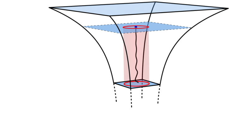
We can also imagine the situation in which one has forced motion from the boundary perspective due to an external force. This can be easily realized in from the bulk perspective by turning on a world-volume $U(1)$ gauge field on the flavor branes. Since the endpoint of the string is charged under this $U(1)$, this amounts to adding to the action the minimal coupling $S=S_{\text{NG}}+S_{\text{EM}}$, where

$$S_{\text{EM}}=\int_{\partial\Sigma}dt\left(A_{t}+A_{x}\dot{X}\right)\,.$$

(47)

This will exert the desired force on our Brownian particle. However, this is just a boundary term, so it will not play any role for the string dynamics in the bulk, other than modify the boundary condition. This will be important in section 4.3 for the computation of the admittance. For now we will pay no attention to this part of the action.

The equation of motion coming from action (46) is

$$\partial_{z}\left[\frac{f(z)^{3}}{z^{2}}X^{\prime}\right]-\partial_{t}\left[\frac{f(z)}{z^{2}}\dot{X}\right]+\frac{f(z)}{z^{2}}H^{2}X=0\,.$$

(48)

Now, given that the background (10) is invariant under time translations, we can perform a Fourier decomposition

$$X(t,z)\sim e^{-i\omega t}g_{\omega}(z)\,.$$

(49)

Plugging (49) in (48) we obtain the following equation for the modes

$$\partial_{z}\left[\frac{1}{z^{2}}\left(1-\frac{H^{2}z^{2}}{4}\right)^{3}g_{\omega}^{\prime}(z)\right]+\frac{\omega^{2}+H^{2}}{z^{2}}\left(1-\frac{H^{2}z^{2}}{4}\right)g_{\omega}(z)=0\,.$$

(50)

The two linearly independent solutions are

	$\displaystyle g^{(\text{in})}_{\omega}{(z)}=\frac{(4-4i\omega z+H^{2}z^{2})}{(4-H^{2}z^{2})}e^{i2\omega\,\mathrm{arctanh}(Hz/2)/H}\,,$		(51)
	$\displaystyle g^{(\text{out})}_{\omega}{(z)}=g^{(in)}_{\omega}{(z)}^{*}\,,$		(52)

where the superscripts $(\text{in})/(\text{out})$ refer to incoming and outgoing waves with respect to the bulk horizon. To see this notice that, around the unperturbed solution $X=0$, the worldsheet metric (45) can be written as

$$ds^{2}_{\text{ws}}=\frac{L^{2}}{z^{2}}f(z)\left[-f(z)dt^{2}+\frac{dz^{2}}{f(z)}\right]\,,$$

(53)

which is conformal to a metric of the “black hole form”. This suggests that we can define a tortoise coordinate as

$$z_{*}=-\int\frac{dz}{f(z)}=-\frac{2}{H}\mathrm{arctanh}{(Hz/2)}\,,$$

(54)

where the horizon lies now at $z_{*}\to-\infty$. In terms of this coordinate, the solutions above take the more familiar form

	$\displaystyle X^{(\text{in})}(t,z)\propto e^{-i\omega(t+z_{*})}\,,$		(55)
	$\displaystyle X^{(\text{out})}(t,z)\propto e^{-i\omega(t-z_{*})}\,.$		(56)

Note also that, in the near horizon limit, the action (46) can be written as

$$S_{\text{NG}}\propto\int dtdz_{*}\left[X^{\prime 2}-\dot{X}^{2}-H^{2}X^{2}\right]\,,$$

(57)

where now primes denote derivatives with respect to the tortoise coordinate $z_{*}$. This is precisely the form of the action of a Klein-Gordon scalar field in Minkowski space with an inverted harmonic potential.

Away from the near horizon regime, however, the action (46) describes the dynamics of a scalar field $X(t,z)$ in a curved background (53). Standard quantization in a curved space [1, 2] leads to a mode expansion of the form

$$X(t,z)=\int_{0}^{\infty}\frac{d\omega}{2\pi}[a_{\omega}u_{\omega}(t,z)+a_{\omega}^{\dagger}u_{\omega}(t,z)^{*}]\,,$$

(58)

where the functions $u_{\omega}$ correspond to a normalized basis of positive-frequency modes. These modes can be expressed as a linear combination of ingoing and outgoing waves with arbitrary coefficients,

$$u_{\omega}{(t,z)}=A_{\omega}[g^{(in)}_{\omega}{(z)}+B_{\omega}g^{(out)}_{\omega}{(z)}]e^{-i\omega t}\,.$$

(59)

The constant $B_{\omega}$ is fixed through the boundary condition at $z=z_{m}$. In particular, in the absence of external forces one imposes a Neumann boundary condition

$$\partial_{z}u_{\omega}(t,z)|_{z=z_{m}}=0\,,$$

(60)

which leads to

$$B_{\omega}=-e^{4i\omega\,\mathrm{arctanh}(Hz_{m}/2)/H}\,.$$

(61)

In particular, notice that this is a pure phase $\sim e^{i\theta}$. Then, outgoing and ingoing modes have the same amplitude and this implies that the black hole, which emits Hawking radiation, can be in thermal equilibrium [127]. On the other hand, the constant $A_{\omega}$ is obtained by requiring the normalization of the modes through the standard Klein-Gordon inner product. After some algebra (see Appendix B) we get

$$A_{\omega}=\left(\frac{\pi}{\sqrt{\lambda}\omega(H^{2}+\omega^{2})}\right)^{\!\!\frac{1}{2}}\,.$$

(62)

The rest of this section is organized as follows. In 4.2 we compute the two-point functions of position and momentum, and from these we extract the displacement squared $\left\langle s(t)^{2}\right\rangle$ and the random force strength $\kappa(\omega)$, respectively. In 4.3 we determine the admittance $\mu(\omega)$ and the friction kernel $\gamma(\omega)$ by measuring the response $\left\langle p(\omega)\right\rangle$ due to an external force. Finally, in 4.4 we comment on the proposed Langevin equation (22) and the time scales characterizing the evolution of the Brownian particle.

In the semi-classical treatment, string modes are thermally excited by Hawking radiation emitted by the worldsheet horizon. In particular, assuming that the state of the embedding fields is the usual Hartle-Hawking (or Euclidean) vacuum [128, 129], these modes follow the standard Bose-Einstein distribution:

$$\langle a_{\omega}^{\dagger}a_{\omega^{\prime}}\rangle=\frac{2\pi\delta(\omega-\omega^{\prime})}{e^{\beta\omega}-1}\,,\qquad\langle a_{\omega}a_{\omega^{\prime}}\rangle=\langle a^{\dagger}_{\omega}a^{\dagger}_{\omega^{\prime}}\rangle=0\,,$$

(63)

where

$$\beta=\frac{1}{T_{\text{dS}}}=\frac{2\pi}{H}\,.$$

(64)

The position of the particle is identified as the string endpoint at $z=z_{m}$:

$$x(t)=X(t,z_{m})=\int_{0}^{\infty}\frac{d\omega}{2\pi}[a_{\omega}u_{\omega}(t,z_{m})+a_{\omega}^{\dagger}u_{\omega}^{*}(t,z_{m})]\,.$$

(65)

Substituting our solution for the modes into the above expression, we find

$$x(t)=-2iz_{m}\int_{0}^{\infty}\frac{d\omega}{2\pi}\left[a_{\omega}\omega A_{\omega}\left(\frac{2+Hz_{m}}{2-Hz_{m}}\right)^{i\frac{\omega}{H}}e^{-i\omega t}+\mathrm{h.c.}\right]\,,$$

(66)

where $A_{\omega}$ is the normalization constant given in (62). Next, we compute the 2-point function $\langle x(t)x(0)\rangle$. This has the usual IR divergence that comes from the zero-point energy, which exists even in the zero temperature limit $\beta\to\infty$. To avoid this, we regularize the correlator by implementing the normal ordering ${:\!a_{\omega}a_{\omega}^{\dagger}\!:}\equiv{:\!a_{\omega}^{\dagger}a_{\omega}\!:}=a_{\omega}^{\dagger}a_{\omega}$. This yields¹⁷¹⁷ 17 We have to keep in mind that normal-ordering does not respect the KMS conditions except in the classical limit. A different way to treat this divergence is by means of the canonical correlator— see appendix E for details.

$$\langle:\!x(t)x(0)\!:\rangle=\frac{\sqrt{\lambda}}{\pi^{2}m^{2}}\int_{0}^{\infty}d\omega\frac{\cos{(\omega t)}}{e^{\beta\omega}-1}\frac{\omega}{H^{2}+\omega^{2}}\,.$$

(67)

From this correlator, we can compute the displacement squared. After some straightforward algebra, we obtain

$$\langle:\!s^{2}(t)\!:\rangle=\frac{4\sqrt{\lambda}}{\pi^{2}m^{2}}\int_{0}^{\infty}d\omega\frac{\sin^{2}{(\omega t/2)}}{e^{\beta\omega}-1}\frac{\omega}{H^{2}+\omega^{2}}\,,$$

(68)

where in the process we used the identity $1-\cos{(x)}=2\sin^{2}{(x/2)}$. Expression (68) can be written in terms of a dimensionless integral as follows:

$$\langle:\!s^{2}{(t)}\!:\rangle=\frac{\sqrt{\lambda}}{\pi^{4}m^{2}}\int_{0}^{\infty}dx\frac{\sin^{2}{(\frac{Ht}{4\pi}x)}}{e^{x}-1}\frac{x}{1+\frac{x^{2}}{4\pi^{2}}}\,.$$

(69)

Notice that the displacement squared vanishes in two limits: $m\rightarrow\infty$ and $H\rightarrow 0$. In the first case, the particle is infinitely heavy and, therefore, we do not expect it to undergo Brownian motion; in the second case, the temperature vanishes and the particle is not expected to undergo Brownian motion either.

We explicitly evaluate the integral in (69) in appendix C. The final result is

	$\displaystyle\langle:\!s^{2}{(t)}\!:\rangle=\frac{\sqrt{\lambda}}{2\pi^{2}m^{2}}\big[2\gamma_{E}-e^{Ht}\mathrm{Ei}{(-Ht)}-e^{-Ht}\mathrm{Ei}{(Ht)}$
	$\displaystyle\qquad\qquad\qquad\qquad\qquad+(e^{Ht}+e^{-Ht})\log{(1-e^{-Ht})}+Hte^{-Ht}\big]\,,$		(70)

where $\gamma_{E}$ is the Euler-Mascheroni constant and ${\rm Ei}(z)$ is the exponential integral. At early times, we recover the anticipated ballistic regime,

$$\langle:\!s^{2}{(t)}\!:\rangle\approx v_{0}^{2}t^{2}+\mathcal{O}((Ht)^{4})\,,$$

(71)

where the constant $v_{0}$ is given by

$$v_{0}^{2}=\left(\frac{\sqrt{\lambda}H^{2}}{4\pi^{2}m^{2}}\right)\left(\frac{7}{6}-2\gamma_{E}\right)\,.$$

(72)

However, in the scaling of (72), there is an extra factor of order $\sim\mathcal{O}(\sqrt{\lambda}T_{dS}/m)$ in comparison to the expected behavior in thermal field theories. This peculiar behavior implies that the energy transferred in a single collision is $\sim\sqrt{\lambda}T_{\text{dS}}^{2}/m$, instead of instead of the standard $\sim T_{\text{dS}}$ predicted by the equipartition theorem. We will comment more on this point in appendix D, where we explicitly compute the distribution of velocities of the Brownian particle.

In terms of $v_{0}$, the displacement squared takes the form

	$\displaystyle\langle:\!s^{2}{(t)}\!:\rangle=\frac{v_{0}^{2}}{H^{2}\left(\frac{7}{12}-\gamma_{E}\right)}\big[2\gamma_{E}-e^{Ht}\mathrm{Ei}{(-Ht)}-e^{-Ht}\mathrm{Ei}{(Ht)}$
	$\displaystyle\qquad\qquad\qquad\qquad\qquad\qquad\quad+(e^{Ht}+e^{-Ht})\log{(1-e^{-Ht})}+Hte^{-Ht}\big]\,.$		(73)

In the late time regime, we find that the displacement squared does, indeed, approach a constant value:

$$\langle:\!s^{2}{(t)}\!:\rangle=\frac{v_{0}^{2}}{H^{2}}\frac{(2\gamma_{E}-1)}{(\frac{7}{12}-\gamma_{E})}+\mathcal{O}((Ht)^{-2})\,.$$

(74)

Since the Brownian particle is very massive, its motion is non-relativistic ($v_{0}\ll 1$) and, in the limit above, $\langle:\!s^{2}{(t)}\!:\rangle$ is in general smaller than $1/H^{2}$. If we take $v_{0}$ to be at most one order of magnitude smaller than the speed of light then, according to (74), the furthest the particle can go is approximately halfway to the horizon. Notice that this is what the observer at $r=0$ sees, as the coordinate $t$ measures the time according to such an observer. Intuitively, the fact that the particle does not actually reach the horizon is due to the fact that it interacts with more and more Hawking quanta as it approaches the horizon. At the equilibrium position then, the random kicks counteract the gravitational repulsion due to the de Sitter metric.

References

- (1) N. D. Birrell and P. C. W. Davies, “Quantum Fields In Curved Space,” Cambridge Univ. Pr., UK (1982) 340p.
- (2) R. M. Wald, “Quantum field theory in curved space-time and black hole thermodynamics,” Chicago Univ. Pr., USA (1994) 205p.
- (3) S. B. Giddings, “Black hole information, unitarity, and nonlocality,” Phys. Rev. D 74, 106005 (2006) [hep-th/0605196].
- (4) S. D. Mathur, “The Information paradox: A Pedagogical introduction,” Class. Quant. Grav. 26, 224001 (2009) [arXiv:0909.1038 [hep-th]].
- (5) T. Banks, “TASI Lectures on Holographic Space-Time, SUSY and Gravitational Effective Field Theory,” arXiv:1007.4001 [hep-th].
- (6) A. Almheiri, D. Marolf, J. Polchinski and J. Sully, “Black Holes: Complementarity or Firewalls?,” JHEP 1302, 062 (2013) [arXiv:1207.3123 [hep-th]].
- (7) S. L. Braunstein, “Black hole entropy as entropy of entanglement, or it’s curtains for the equivalence principle,” arXiv:0907.1190v1 [quant-ph], published as S. L. Braunstein, S. Pirandola and K. Życzkowski, “Better Late than Never: Information Retrieval from Black Holes,” Physical Review Letters 110, 101301 (2013) [arXiv:0907.1190v3 [quant-ph]].
- (8) A. Strominger, “The dS / CFT correspondence,” JHEP 0110, 034 (2001) [hep-th/0106113].
- (9) B. McInnes, “The dS / CFT correspondence and the big smash,” JHEP 0208, 029 (2002) [hep-th/0112066].
- (10) A. Strominger, “Inflation and the dS / CFT correspondence,” JHEP 0111, 049 (2001) [hep-th/0110087].
- (11) J. M. Maldacena, “The Large N limit of superconformal field theories and supergravity,” Adv. Theor. Math. Phys. 2, 231 (1998), Int. J. Theor. Phys. 38, 1113 (1999), [hep-th/9711200].
- (12) S. S. Gubser, I. R. Klebanov and A. M. Polyakov, “Gauge theory correlators from non-critical string theory,” Phys. Lett. B 428, 105 (1998) [arXiv:hep-th/9802109].
- (13) E. Witten, “Anti-de Sitter space and holography,” Adv. Theor. Math. Phys. 2, 253 (1998) [arXiv:hep-th/9802150].
- (14) T. Banks, W. Fischler, S. H. Shenker and L. Susskind, “M theory as a matrix model: A Conjecture,” Phys. Rev. D 55, 5112 (1997) [hep-th/9610043].
- (15) W. Fischler and L. Susskind, “Holography and cosmology,” hep-th/9806039.
- (16) M. Alishahiha, A. Karch, E. Silverstein and D. Tong, “The dS/dS correspondence,” AIP Conf. Proc. 743, 393 (2005) [hep-th/0407125].
- (17) B. Freivogel, Y. Sekino, L. Susskind and C. -P. Yeh, “A Holographic framework for eternal inflation,” Phys. Rev. D 74, 086003 (2006) [hep-th/0606204].
- (18) Y. Sekino and L. Susskind, “Census Taking in the Hat: FRW/CFT Duality,” Phys. Rev. D 80, 083531 (2009) [arXiv:0908.3844 [hep-th]].
- (19) X. Dong, B. Horn, E. Silverstein and G. Torroba, “Micromanaging de Sitter holography,” Class. Quant. Grav. 27, 245020 (2010) [arXiv:1005.5403 [hep-th]].
- (20) T. Banks, “Holographic Space-Time: The Takeaway,” arXiv:1109.2435 [hep-th].
- (21) T. Banks and W. Fischler, “Holographic Theories of Inflation and Fluctuations,” arXiv:1111.4948 [hep-th].
- (22) T. Banks and W. Fischler, “Holographic Theory of Accelerated Observers, the S-matrix, and the Emergence of Effective Field Theory,” arXiv:1301.5924 [hep-th].
- (23) T. Banks and W. Fischler, “Holographic Space-time and Newton’s Law,” arXiv:1310.6052 [hep-th].
- (24) A. Buchel, “Gauge / gravity correspondence in accelerating universe,” Phys. Rev. D 65, 125015 (2002) [hep-th/0203041].
- (25) A. Buchel, P. Langfelder and J. Walcher, “On time dependent backgrounds in supergravity and string theory,” Phys. Rev. D 67, 024011 (2003) [hep-th/0207214].
- (26) O. Aharony, M. Fabinger, G. T. Horowitz and E. Silverstein, “Clean time dependent string backgrounds from bubble baths,” JHEP 0207, 007 (2002) [hep-th/0204158].
- (27) V. Balasubramanian and S. F. Ross, “The Dual of nothing,” Phys. Rev. D 66, 086002 (2002) [hep-th/0205290].
- (28) R. -G. Cai, “Constant curvature black hole and dual field theory,” Phys. Lett. B 544, 176 (2002) [hep-th/0206223].
- (29) E. Silverstein and D. Tong, “Scalar speed limits and cosmology: Acceleration from D-cceleration,” Phys. Rev. D 70, 103505 (2004) [hep-th/0310221].
- (30) S. F. Ross and G. Titchener, “Time-dependent spacetimes in AdS/CFT: Bubble and black hole,” JHEP 0502, 021 (2005) [hep-th/0411128].
- (31) V. Balasubramanian, K. Larjo and J. Simon, “Much ado about nothing,” Class. Quant. Grav. 22, 4149 (2005) [hep-th/0502111].
- (32) M. Alishahiha, A. Karch and E. Silverstein, “Hologravity,” JHEP 0506, 028 (2005) [hep-th/0504056].
- (33) B. Freivogel, V. E. Hubeny, A. Maloney, R. C. Myers, M. Rangamani and S. Shenker, “Inflation in AdS/CFT,” JHEP 0603, 007 (2006) [hep-th/0510046].
- (34) A. Buchel, “Inflation on the resolved warped deformed conifold,” Phys. Rev. D 74, 046009 (2006) [hep-th/0601013].
- (35) T. Hirayama, “A Holographic dual of CFT with flavor on de Sitter space,” JHEP 0606, 013 (2006) [hep-th/0602258].
- (36) K. Ghoroku, M. Ishihara and A. Nakamura, “Gauge theory in de Sitter space-time from a holographic model,” Phys. Rev. D 74, 124020 (2006) [hep-th/0609152].
- (37) J. He and M. Rozali, “On bubbles of nothing in AdS/CFT,” JHEP 0709, 089 (2007) [hep-th/0703220 [HEP-TH]].
- (38) K. Ghoroku, M. Ishihara and A. Nakamura, “Flavor quarks in AdS4 and gauge/gravity correspondence,” Phys. Rev. D 75, 046005 (2007) [hep-th/0612244].
- (39) J. A. Hutasoit, S. P. Kumar and J. Rafferty, “Real time response on dS(3): The Topological AdS Black Hole and the Bubble,” JHEP 0904, 063 (2009) [arXiv:0902.1658 [hep-th]].
- (40) D. Marolf, M. Rangamani and M. Van Raamsdonk, “Holographic models of de Sitter QFTs,” Class. Quant. Grav. 28, 105015 (2011) [arXiv:1007.3996 [hep-th]].
- (41) M. Li and Y. Pang, “Holographic de Sitter Universe,” JHEP 1107, 053 (2011) [arXiv:1105.0038 [hep-th]].
- (42) J. Erdmenger, K. Ghoroku and R. Meyer, “Holographic (De)confinement Transitions in Cosmological Backgrounds,” Phys. Rev. D 84, 026004 (2011) [arXiv:1105.1776 [hep-th]].
- (43) K. Ghoroku and A. Nakamura, “Holographic Friedmann equation and N=4 supersymmetric Yang-Mills theory,” Phys. Rev. D 87, no. 6, 063507 (2013) [arXiv:1212.2304 [hep-th]].
- (44) A. Buchel and D. A. Galante, “Cascading gauge theory on dS4 and String Theory Landscape,” [arXiv:1310.1372 [hep-th]].
- (45) W. Fischler, S. Kundu and J. F. Pedraza, “Entanglement and out-of-equilibrium dynamics in holographic models of de Sitter QFTs,” arXiv:1311.5519 [hep-th].
- (46) R. Emparan, “AdS membranes wrapped on surfaces of arbitrary genus,” Phys. Lett. B 432 (1998) 74 [hep-th/9804031].
- (47) D. Birmingham, “Topological black holes in Anti-de Sitter space,” Class. Quant. Grav. 16 (1999) 1197 [hep-th/9808032].
- (48) R. Emparan, “AdS/CFT duals of topological black holes and the entropy of zero energy states,” JHEP 9906 (1999) 036 [hep-th/9906040].
- (49) G. W. Gibbons and S. W. Hawking, “Cosmological Event Horizons, Thermodynamics, and Particle Creation,” Phys. Rev. D15 (1977) 2738-2751.
- (50) T. S. Bunch and P. C. W. Davies, “Quantum Field Theory in de Sitter Space: Renormalization by Point Splitting,” Proc. Roy. Soc. Lond. A360 (1978) 117-134.
- (51) S. -J. Rey and J. -T. Yee, “Macroscopic strings as heavy quarks in large N gauge theory and anti-de Sitter supergravity,” Eur. Phys. J. C 22, 379 (2001) [hep-th/9803001].
- (52) C. P. Herzog, A. Karch, P. Kovtun, C. Kozcaz and L. G. Yaffe, “Energy loss of a heavy quark moving through N = 4 supersymmetric Yang-Mills plasma,” JHEP 0607, 013 (2006) [arXiv:hep-th/0605158].
- (53) S. S. Gubser, “Drag force in AdS/CFT,” Phys. Rev. D 74, 126005 (2006) [arXiv:hep-th/0605182].
- (54) J. de Boer, V. E. Hubeny, M. Rangamani and M. Shigemori, “Brownian motion in AdS/CFT,” JHEP 0907, 094 (2009) [arXiv:0812.5112 [hep-th]].
- (55) D. T. Son and D. Teaney, “Thermal Noise and Stochastic Strings in AdS/CFT,” JHEP 0907, 021 (2009) [arXiv:0901.2338 [hep-th]].
- (56) S. S. Gubser, “Momentum fluctuations of heavy quarks in the gauge-string duality,” Nucl. Phys. B 790 (2008) 175 [arXiv:hep-th/0612143].
- (57) J. Casalderrey-Solana and D. Teaney, “Transverse momentum broadening of a fast quark in a Yang Mills plasma,” JHEP 0704 (2007) 039 [arXiv:hep-th/0701123].
- (58) B. L. Hu and A. Matacz, “Quantum Brownian motion in a bath of parametric oscillators: A Model for system - field interactions,” Phys. Rev. D 49, 6612 (1994) [gr-qc/9312035].
- (59) M. -T. Jaekel and S. Reynaud, “Movement and fluctuations of the vacuum,” Rept. Prog. Phys. 60, 863 (1997) [quant-ph/9706035].
- (60) A. Fingerle, “Relativistic fluctuation theorems,” Comptes Rendus Physique 8, 696 (2007) [arXiv:0705.3115 [gr-qc]].
- (61) Z. Haba, “Relativistic diffusion with friction on a pseudoriemannian manifold,” Class. Quant. Grav. 27, 095021 (2010) [arXiv:0909.2880 [gr-qc]].
- (62) S. Iso, Y. Yamamoto and S. Zhang, “Stochastic Analysis of an Accelerated Charged Particle -Transverse Fluctuations-,” Phys. Rev. D 84, 025005 (2011) [arXiv:1011.4191 [hep-th]].
- (63) S. Kolekar and T. Padmanabhan, “Drift, Drag and Brownian motion in the Davies-Unruh bath,” Phys. Rev. D 86, 104057 (2012) [arXiv:1205.0258 [gr-qc]].
- (64) G. Rigopoulos, “Fluctuation-dissipation and equilibrium for scalar fields in de Sitter,” arXiv:1305.0229 [astro-ph.CO].
- (65) N. Oshita, K. Yamamoto and S. Zhang, “Thermal property in Brownian motion of a particle coupled to vacuum fluctuations,” arXiv:1403.5028 [gr-qc].
- (66) E. Caceres, M. Chernicoff, A. Guijosa and J. F. Pedraza, “Quantum Fluctuations and the Unruh Effect in Strongly-Coupled Conformal Field Theories,” JHEP 1006, 078 (2010) [arXiv:1003.5332 [hep-th]].
- (67) G. C. Giecold, E. Iancu and A. H. Mueller, “Stochastic trailing string and Langevin dynamics from AdS/CFT,” JHEP 0907, 033 (2009) [arXiv:0903.1840 [hep-th]].
- (68) J. Casalderrey-Solana, K. -Y. Kim and D. Teaney, “Stochastic String Motion Above and Below the World Sheet Horizon,” JHEP 0912, 066 (2009) [arXiv:0908.1470 [hep-th]].
- (69) A. N. Atmaja, J. de Boer and M. Shigemori, “Holographic Brownian Motion and Time Scales in Strongly Coupled Plasmas,” Nucl. Phys. B 880, 23 (2014) [arXiv:1002.2429 [hep-th]].
- (70) S. R. Das, T. Nishioka and T. Takayanagi, “Probe Branes, Time-dependent Couplings and Thermalization in AdS/CFT,” JHEP 1007, 071 (2010) [arXiv:1005.3348 [hep-th]].
- (71) U. Gursoy, E. Kiritsis, L. Mazzanti and F. Nitti, “Langevin diffusion of heavy quarks in non-conformal holographic backgrounds,” JHEP 1012, 088 (2010) [arXiv:1006.3261 [hep-th]].
- (72) H. Ebrahim and M. Headrick, “Instantaneous Thermalization in Holographic Plasmas,” arXiv:1010.5443 [hep-th].
- (73) S. Caron-Huot, P. M. Chesler and D. Teaney, “Fluctuation, dissipation, and thermalization in non-equilibrium AdS5 black hole geometries,” Phys. Rev. D 84, 026012 (2011) [arXiv:1102.1073 [hep-th]].
- (74) E. Kiritsis, L. Mazzanti and F. Nitti, “Dressed spectral densities for heavy quark diffusion in holographic plasmas,” J. Phys. G 39, 054003 (2012) [arXiv:1111.1008 [hep-th]].
- (75) W. Fischler, J. F. Pedraza and W. Tangarife Garcia, “Holographic Brownian Motion in Magnetic Environments,” JHEP 1212, 002 (2012) [arXiv:1209.1044 [hep-th]].
- (76) D. Tong and K. Wong, “Fluctuation and Dissipation at a Quantum Critical Point,” Phys. Rev. Lett. 110, no. 6, 061602 (2013) [arXiv:1210.1580 [hep-th]].
- (77) M. Edalati, J. F. Pedraza and W. Tangarife Garcia, “Quantum Fluctuations in Holographic Theories with Hyperscaling Violation,” Phys. Rev. D 87, no. 4, 046001 (2013) [arXiv:1210.6993 [hep-th]].
- (78) A. N. Atmaja, “Holographic Brownian Motion in Two Dimensional Rotating Fluid,” JHEP 1304, 021 (2013) [arXiv:1212.5319 [hep-th]].
- (79) J. Sadeghi, F. Pourasadollah and H. Vaez, “Holograghic Brownian motion in three dimensional Gödel black hole,” arXiv:1308.2483 [hep-th].
- (80) A. N. Atmaja, “Effective Mass of Holographic Brownian Particle in Rotating Plasma,” arXiv:1308.3014 [hep-th].
- (81) P. Banerjee and B. Sathiapalan, “Holographic Brownian Motion in 1+1 Dimensions,” arXiv:1308.3352 [hep-th].
- (82) D. Giataganas and H. Soltanpanahi, “Universal Properties of the Langevin Diffusion Coefficients,” Phys. Rev. D 89, 026011 (2014) [arXiv:1310.6725 [hep-th]].
- (83) C. -P. Yeh, J. -T. Hsiang and D. -S. Lee, “Holographic Approach to Nonequilibrium Dynamics of Moving Mirrors Coupled to Quantum Critical Theories,” Phys. Rev. D 89, 066007 (2014) [arXiv:1310.8416 [hep-th]].
- (84) E. Kiritsis, L. Mazzanti and F. Nitti, “The confining trailing string,” JHEP 1402, 081 (2014) [arXiv:1311.2611 [hep-th]].
- (85) S. Chakrabortty, S. Chakraborty and N. Haque, “Brownian motion in strongly coupled, anisotropic Yang-Mills plasma: A holographic approach,” arXiv:1311.5023 [hep-th].
- (86) J. Sadeghi, B. Pourhassan and F. Pourasadollah, “Holograghic Brownian motion in dimensional hairy black holes,” Eur. Phys. J. C 74, 2793 (2014) [arXiv:1312.4906 [hep-th]].
- (87) D. Giataganas and H. Soltanpanahi, “Heavy Quark Diffusion in Strongly Coupled Anisotropic Plasmas,” arXiv:1312.7474 [hep-th].
- (88) J. Sadeghi and F. Pourasadollah, “Langevin diffusion in holographic backgrounds with hyperscaling violation,” arXiv:1403.2192 [hep-th].
- (89) D. Marolf, M. Rangamani and T. Wiseman, “Holographic thermal field theory on curved spacetimes,” arXiv:1312.0612 [hep-th].
- (90) C. Fefferman, C. R. Graham, Conformal invariants, in Élie Cartan et les Mathématiques d’Aujourd’hui, (Astérisque, 1985), 95.
- (91) S. de Haro, S. N. Solodukhin and K. Skenderis, “Holographic reconstruction of spacetime and renormalization in the AdS/CFT correspondence,” Commun. Math. Phys. 217 (2001) 595 [arXiv:hep-th/0002230].
- (92) K. Skenderis, “Asymptotically anti-de Sitter spacetimes and their stress energy tensor,” Int. J. Mod. Phys. A 16, 740 (2001) [arXiv:hep-th/0010138].
- (93) K. Skenderis, “Lecture notes on holographic renormalization,” Class. Quant. Grav. 19 (2002) 5849 [arXiv:hep-th/0209067].
- (94) E. Mottola, “Particle Creation in de Sitter Space,” Phys. Rev. D31(1985) 754.
- (95) B. Allen, “Vacuum States in de Sitter Space,” Phys. Rev. D32 (1985) 3136.
- (96) R. Brown, “A brief account of microscopical observations made in the months of June, July and August, 1827, on the particles contained in the pollen of plants; and on the general existence of active molecules in organic and inorganic bodies,” Philos. Mag. 4, 161 (1828); reprinted in Edinburgh New Philos. J. 5, 358 (1928).
- (97) G. E. Uhlenbeck and L. S. Ornstein, “On The Theory Of The Brownian Motion,” Phys. Rev. 36, 823 (1930).
- (98) S. Chandrasekhar, “Stochastic problems in physics and astronomy,” Rev. Mod. Phys. 15, 1 (1943).
- (99) M. C. Wang and G. E. Uhlenbeck, “On the Theory of the Brownian Motion II,” Rev. Mod. Phys. 17, 323 (1945).
- (100) S. Weinberg, Gravitation and Cosmology: Principles and Applications of the General Theory of Relativity (John Wiley & Sons, New York, 1972).
- (101) H. Mori, “Transport, collective motion, and Brownian motion,” Prog. Theor. Phys. 33, 423 (1965).
- (102) R. Kubo, “The fluctuation-dissipation theorem,” Rep. Prog. Phys. 29, 255-284 (1966).
- (103) R. Stratton, “Diffusion of Hot and Cold Electrons in Semiconductor Barriers,” Phys. Rev. 126, 2002 (1962); “Semiconductor current-flow equations (diffusion and degeneracy),” IEEE Trans. Electr. Devices 19, 1288-1292 (1972).
- (104) J. D. Gassaway, “A note on the semiconductor current flow equations,” IEEE Trans. Electr. Devices 18, 175-178 (1971).
- (105) A. H. Marshak and D. Assaf III, “A generalized Einstein relation for semiconductors,” Solid-State Electron. 16, 675-679 (1973).
- (106) G. Baccarani, “On the diffusion current in heavily doped semiconductors,” Solid-State Electron. 18, 469-470 (1975).
- (107) P. T. Landsberg and S. A. Hope, “Diffusion currents in semiconductors,” Solid-State Electron. 19, 173-174 (1976); “Two formulations of semiconductor transport equations,” Solid-State Electron. 20, 421-429 (1977).
- (108) M. Büttiker and R. Landauer, Nonlinear Phenomena at Phase Transitions and Instabilities (Plenum Press, New York, 1982, pp 111-143).
- (109) N.G. Van Kampen “Diffusion in inhomogeneous media,” J. Phys. Chem. Solids 49, 673-677 (1988).
- (110) M. E. Widder and U. M. Titulaer, “Brownian motion in a medium with inhomogeneous temperature,” Physica A 154, 452–466 (1989).
- (111) R. Landauer, “Statistical physics of machinery: forgotten middle-ground,” Physica A 194, 551-562 (1993).
- (112) Y. Sagi et al., “Observation of Anomalous Diffusion and Fractional Self-Similarity in One Dimension,” Phys. Rev. Lett. 108, 093002 (2012).
- (113) I. Bronstein et al., “Transient Anomalous Diffusion of Telomeres in the Nucleus of Mammalian Cells,” Phys. Rev. Lett. 103, 018102 (2009).
- (114) B. M. Regne et al., “Anomalous Diffusion of Single Particles in Cytoplasm,” Biophys. J. 104, 1652-1660 (2013).
- (115) J.-H. Jeon et al., “Anomalous diffusion and power-law relaxation of the time averaged mean squared displacement in worm-like micellar solutions,” New J. Phys. 15 045011 (2013).
- (116) M. Chernicoff, J. A. Garcia, A. Guijosa and J. F. Pedraza, “Holographic Lessons for Quark Dynamics,” J. Phys. G G 39, 054002 (2012) [arXiv:1111.0872 [hep-th]].
- (117) J. L. Hovdebo, M. Kruczenski, D. Mateos, R. C. Myers and D. J. Winters, “Holographic mesons: Adding flavor to the AdS/CFT duality,” Int. J. Mod. Phys. A 20, 3428 (2005).
- (118) M. Chernicoff, A. Guijosa and J. F. Pedraza, “The Gluonic Field of a Heavy Quark in Conformal Field Theories at Strong Coupling,” JHEP 1110, 041 (2011) [arXiv:1106.4059 [hep-th]].
- (119) C. A. Agon, A. Guijosa and J. F. Pedraza, “Radiation and a dynamical UV/IR connection in AdS/CFT,” arXiv:1402.5961 [hep-th].
- (120) M. Chernicoff and A. Guijosa, “Acceleration, Energy Loss and Screening in Strongly-Coupled Gauge Theories,” JHEP 0806, 005 (2008) [arXiv:0803.3070 [hep-th]].
- (121) M. Chernicoff, J. A. Garcia and A. Guijosa, “Generalized Lorentz-Dirac Equation for a Strongly-Coupled Gauge Theory,” Phys. Rev. Lett. 102, 241601 (2009) [arXiv:0903.2047 [hep-th]].
- (122) M. Chernicoff, J. A. Garcia and A. Guijosa, “A Tail of a Quark in N=4 SYM,” JHEP 0909, 080 (2009) [arXiv:0906.1592 [hep-th]].
- (123) A. Guijosa and J. F. Pedraza, “Early-Time Energy Loss in a Strongly-Coupled SYM Plasma,” JHEP 1105, 108 (2011) [arXiv:1102.4893 [hep-th]].
- (124) J. Casalderrey-Solana and D. Mateos, “Prediction of a Photon Peak in Relativistic Heavy Ion Collisions,” Phys. Rev. Lett. 102, 192302 (2009) [arXiv:0806.4172 [hep-ph]].
- (125) J. Casalderrey-Solana, D. Fernandez and D. Mateos, “A New Mechanism of Quark Energy Loss,” Phys. Rev. Lett. 104, 172301 (2010) [arXiv:0912.3717 [hep-ph]].
- (126) J. Casalderrey-Solana, D. Fernandez and D. Mateos, “Cherenkov mesons as in-medium quark energy loss,” JHEP 1011, 091 (2010) [arXiv:1009.5937 [hep-th]].
- (127) S. Hemming and E. Keski-Vakkuri, “Hawking radiation from AdS black holes,” Phys. Rev. D 64, 044006 (2001) [arXiv:gr-qc/0005115].
- (128) A. E. Lawrence and E. J. Martinec, “Black hole evaporation along macroscopic strings,” Phys. Rev. D 50, 2680 (1994) [hep-th/9312127, hep-th/9312127].
- (129) V. P. Frolov and D. Fursaev, “Mining energy from a black hole by strings,” Phys. Rev. D 63, 124010 (2001) [hep-th/0012260].
- (130) W. Fischler, P. H. Nguyen, J. F. Pedraza and W. Tangarife, work in progress.
- (131) D. T. Son and A. O. Starinets, “Minkowski space correlators in AdS / CFT correspondence: Recipe and applications,” JHEP 0209, 042 (2002) [hep-th/0205051].
- (132) C. P. Herzog and D. T. Son, “Schwinger-Keldysh propagators from AdS/CFT correspondence,” JHEP 0303, 046 (2003) [hep-th/0212072].
- (133) K. B. Fadafan, H. Liu, K. Rajagopal and U. A. Wiedemann, “Stirring Strongly Coupled Plasma,” Eur. Phys. J. C 61, 553 (2009) [arXiv:0809.2869 [hep-ph]].
- (134) J. M. Maldacena, “Wilson loops in large N field theories,” Phys. Rev. Lett. 80, 4859 (1998) [hep-th/9803002].
- (135) S. -J. Rey, S. Theisen and J. -T. Yee, “Wilson-Polyakov loop at finite temperature in large N gauge theory and anti-de Sitter supergravity,” Nucl. Phys. B 527, 171 (1998) [hep-th/9803135].
- (136) A. Brandhuber, N. Itzhaki, J. Sonnenschein and S. Yankielowicz, “Wilson loops in the large N limit at finite temperature,” Phys. Lett. B 434, 36 (1998) [hep-th/9803137].
- (137) J. Sadeghi and S. Heshmatian, “Screening length of rotating heavy meson from AdS/CFT,” Int. J. Theor. Phys. 49, 1811 (2010).
- (138) H. Liu, K. Rajagopal and U. A. Wiedemann, “Calculating the jet quenching parameter from AdS/CFT,” Phys. Rev. Lett. 97, 182301 (2006) [hep-ph/0605178].