Statistical Error analysis of Nucleon-Nucleon phenomenological potentials
Abstract
Nucleon-Nucleon potentials are commonplace in nuclear physics and are determined from a finite number of experimental data with limited precision sampling the scattering process. We study the statistical assumptions implicit in the standard least squares fitting procedure and apply, along with more conventional tests, a tail sensitive quantile-quantile test as a simple and confident tool to verify the normality of residuals. We show that the fulfillment of normality tests is linked to a judicious and consistent selection of a nucleon-nucleon database. These considerations prove crucial to a proper statistical error analysis and uncertainty propagation. We illustrate these issues by analyzing about 8000 proton-proton and neutron-proton scattering published data. This enables the construction of potentials meeting all statistical requirements necessary for statistical uncertainty estimates in nuclear structure calculations.
Keywords:
NN interaction, One Pion Exchange, Statistical Analysispacs
03.65.Nk,11.10.Gh,13.75.Cs,21.30.Fe,21.45.+vI Introduction
Nucleon-Nucleon potentials are the starting point for many nuclear physics applications [1]. Most of the current information is obtained from np and pp scattering data below pion production threshold and deuteron properties for which abundant experimental data exist. The NN scattering amplitude reads
| (1) | |||||
where depend on energy and angle, and are the single-nucleon Pauli matrices, , , are three unitary orthogonal vectors along the directions of , and , respectively, and (, ) are the final and initial relative nucleon momenta. From these five complex energy and angle dependent quantities 24 measurable cross-sections and polarization asymmetries can be deduced [2]. Inversely, a complete set of experiments can be designed to reconstruct the amplitude at a given energy [3]. The finite amount, precision and limited energy range of the data as well as the many different observables calls for a standard statistical -fit analysis [4, 5]. This approach is subjected to assumptions and applicability conditions that can only be checked a posteriori in order to guarantee the self-consistency of the analysis. Indeed, scattering experiments deal with counting poissonian statistics and for moderately large number of counts a normal distribution is expected. Thus, one hopes that a satisfactory theoretical description can predict a set of N independent observed data given an experimental uncertainty as
| (2) |
with and are independent random normal variables with vanishing mean value and unit variance , implying that . Establishing the validity of Eq. (2) is of utmost importance since it provides a basis for the statistical interpretation of the error analysis. In this work we will study to what extent this normality assumption underlying the validity of the full approach is justified. This will be done by looking at the statistical distribution of the fit residuals of about 8000 np and pp published scattering data collected since 1950. Using the normality test as a necessary requirement we show that it is possible to fulfill Eq. (2) with a high confidence level and high statistics. Furthermore, we discuss the consequences and requirements regarding the evaluation, design and statistical uncertainties of phenomenological nuclear forces. We illustrate our points by determining for the first time a smooth nuclear potential with error bands directly inferred from experiment. We hope that these estimates will be useful for NN potential users interested in quantifying a definite source of error in nuclear structure calculations 11 1 We note that in a Physical Review A editorial [6] the importance of including error estimates in papers involving theoretical evaluations has been stressed..
The history of statistical analyzes of NN scattering data around pion production threshold started in the mid fifties [7] (an account up to 1966 can be traced from Ref. [8]). A modified method was introduced [9] in order to include data without absolute normalization. The steady increase along the years in the number of scattering data and their precision generated mutually incompatible data and hence a rejection criterion was introduced [10, 11, 12] allowing to discard inconsistent data. The upgrading of an ever increasing consistent database poses the question of normality, Eq. (2), of a large number of selected data. The normality of the absolute value of residuals in pp scattering was scrutinized and satisfactorily fulfilled [13, 14] as a necessary consistency condition. The Nijmegen group made 20 years ago an important breakthrough by performing the very first Partial Wave Analysis (PWA) fit with and applying a -rejection criterion. This was possible after including em corrections, vacuum polarization, magnetic moments interaction and a charge-dependent (CD) One Pion Exchange (OPE) potential. With this fixed database further high quality potentials have been steadily generated [15, 16, 17, 18] and applied to nuclear structure calculations. However, high quality potentials, i. e. those whose discrepancies with the data are confidently attributable to statistical fluctuations in the experimental data, have been built and used as if they were error-less. As a natural consequence the computational accuracy to a relative small percentage level has been a goal per se in the solution of the few and many body problem regardless on the absolute accuracy implied by the input of the calculation. While this sets high standards on the numerical methods there is no a priori reason to assume the computational accuracy reflects the realistic physical accuracy and, in fact, it would be extremely useful to determine and identify the main source of uncertainty; one could thus tune the remaining uncertainties to this less demanding level.
It should be noted that the fitting procedure, when applied to limited upper energies, fixes most efficiently the long range piece of the potential which is known to be mainly described by One-Pion-Exchange (OPE) for distances . However, weaker constraints are put in the mid-range region, which is precisely the relevant inter-particle distance operating in the nuclear binding. To date and to the best of our knowledge, the estimation of errors in the nuclear force stemming from the experimental scattering data uncertainties and its consequences for nuclear structure calculations has not been seriously confronted. With this goal in mind we have upgraded the NN database to include all published np and pp scattering data in the period 1950-2013, determining in passing the error in the interaction [19, 20].
The present paper represents an effort towards filling this gap by providing statistical error bands in the NN interaction based directly on the experimental data uncertainties. In order to do so, the specific form of the potential needs to be fixed 22 2 This is also the case in the quantum mechanical inverse scattering problem, which has only unique solutions for specific assumptions on the form of the potential [21] and with the additional requirement that some interpolation of scattering data at non-measured energies is needed. One needs then the information on the bound state energies and their residues in the scattering amplitude. We will likewise impose that the only bound state is the deuteron and reject fits with spurious bound states.. As such, this choice represents a certain bias and hence corresponds to a likely source of systematic error. Based on the previous high quality fits which achieved [15, 16, 17, 18] we have recently raised suspicions on the dominance of such errors with intriguing consequences for the quantitative predictive power of nuclear theory [22, 23, 24]; a rough estimate suggested that NN uncertainties propagate into an unpleasantly large uncertainty of , a figure which has not yet been disputed by an alternative estimate. In view of this surprising finding, there is a pressing need to pin down the input uncertainties more accurately based on a variety of sources 33 3 There is a growing concern on the theoretical determination of nuclear masses from nuclear mean field models with uncertainty evaluation [25] (for a comprehensive discussion see e.g. [26, 27]) echoing the need for uncertainty estimates in a Physical Review A editorial [6] and the Saltelli-Funtowicz seven rules check-list [28].. This work faces the evaluation of statistical errors after checking that the necessary normality conditions of residuals and hence Eq. (2) are confidently fulfilled. From this point of view, the present investigation represents an initial step, postponing a more complete discussion on systematic uncertainties for a future investigation.
The PWA analysis carried out previously by us [22, 23, 24]; was computationally inexpensive due to the use of the simplified -shell potential suggested many years ago by Avilés [29]. This form of potential effectively coarse grains the interaction and drastically reduces the number of integration points in the numerical solution of the Schrödinger equation (see e.g. [30]). However, it is not directly applicable to some of the many numerical methods available on the market to solve the few and many body problem where a smooth potential is required. Therefore, we will analyze the -self consistent database in terms of a more conventional potential form containing the same 21-operators extending the AV18 as we did in[22, 23, 24]. Testing for normality of residuals within a given confidence level for a phenomenological potential is an issue of direct significance to any statistical error analysis and propagation. Actually, we will show that for the fitted observables to the self consistent experimental data base , with quoted uncertainty , (total number of pp and np scattering data), our theoretical fits indeed satisfy that the residuals
| (3) |
follow a normal distribution within a large confidence level. In order to establish this we will use a variety of classical statistical tests [4, 5], such as the Pearson, Kolmogorov-Smirnov (KS), the moments method (MM) and, most importantly, the recently proposed Tail-Sensitive (TS) quantile-quantile test with confidence bands [31]. By comparing with others the TS test turns out to be the most demanding one concerning the confidence bands. Surprisingly, normality tests have only seldom been applied within the present context, so our presentation is intended to be at a comprehensive level. A notable exception is given in Refs. [13, 14] where the moments method in a pp analysis up to and 350 MeV, is used for and 1787 data, respectively, to test that the squared residuals in Eq. (3) follow a -distribution with one degree of freedom. Note, that this is insensitive to the sign of and thus blind to asymmetries in a normal distribution. Here, we test normality of for a total of np and pp data up to MeV.
The paper is organized as follows. In Section II we review the assumptions, the rejecting and fitting process used in our previous works to build the self-consistent database, and expose the main motivation to carry out a normality test of the fit residuals. In Section III we review some of the classical normality tests and a recently proposed tail-sensitive test, which we apply comparatively to the complete as well as the self-consistent database, providing a raison d’être for the rejection procedure. After that, in Section IV we analyze a fit of a potential whose short distance contribution is constructed by a sum of Gaussian functions, with particular attention to the error bar estimation, a viable task since the residuals pass satisfactorily the normality test. Finally in Section V we come to our conclusions and provide some outlook for further work.
II Statistical Considerations
There is a plethora of references on data and error analysis (see e.g. [4, 5]). We will review the fitting approach in such a way that our points can be more easily stated for the general reader.
II.1 Data uncertainties
Scattering experiments are based on counting Poissonian statistics and for moderately large number of counts a normal distribution sets in. In what follows will represent some scattering observable. For a set of independent measurements of different scattering observables experimentalists quote an estimate of the uncertainty so that the true value is contained in the interval with a confidence level. In what follows we assume for simplicity that there are no sources of systematic errors. Actually, when only the pair is provided without specifying the distribution we will assume an underlying normal distribution 44 4 This may not be the most efficient unbiased estimator (see e.g. [4, 5] for a more thorough discussion). Quite generally, the theory for the noise on the specific measurement would involve many considerations on the different experimental setups. In our case the many different experiments makes such an approach unfeasible. There is a possibility that some isolated systematic errors in particular experiments are randomized when considered globally. However, the larger the set the more stringent the corresponding statistical normality test. From this point of view the verification of the normality assumption underlying Eq. (2) proves highly non-trivial., so that
| (4) |
is the probability density of finding measurement .
II.2 Data modeling
The problem of data modeling is to find a theoretical description characterized by some parameters which contain the true value with a given confidence level characterized by a bounded p-dimensional manifold in the space of parameters . For a normal distribution the probability of finding any of the (independent ) measurements , assuming that are the true parameters, is given by
| (5) |
Thus the joined probability density is
| (6) | |||||
where . In such a case the maximum likelihood method [4, 5] corresponds to take the as a figure of merit given by
| (7) |
and look for the minimum in the fitting parameters ,
| (8) |
Our theoretical estimate of after the fit is given by
| (9) |
Expanding around the minimum one has
| (10) |
where the error matrix is defined as the inverse of the Hessian matrix evaluated at the minimum
| (11) |
Finally, the correlation matrix between two fitting parameters and is given by
| (12) |
We compute the error of the parameter as
| (13) |
Error propagation of an observable is computed as
| (14) |
The resulting residuals of the fit are defined as
| (15) |
Assuming normality of residuals is now crucial for an statistical interpretation of the confidence level, since then follows a -distribution. One useful application of the previous result is that we can replicate the experimental data by using Eq. (2) and in such a case . For a large number of data with -parameters one has, with a or confidence level, the mean value and most likely value nearly coincide, so that one has and thus as a random variable we have
| (16) |
where is the number of degrees of freedom. The goodness of fit is defined in terms of this confidence interval. However, the -test has a sign ambiguity for every single residual given that is a symmetry of the test. From this point of view the verification of normality is a more demanding requirement 55 5 One can easily see that for a set of normally distributed data , while does not follow that distribution, would pass a -test..
Thus a necessary condition for a least-squares fit with meaningful results is the residuals to follow a normal distribution with mean zero and variance one, i.e. . It should be noted that a model for the noise need not be normal, but it must be a known distribution such that the residuals do indeed follow such distribution 66 6 In this case the merit figure to minimize would be For instance in Ref. [32], dealing with scattering a Lorentz distribution arose as a self consistent assumption..
II.3 Data selection
The first and most relevant problem one has to confront in the phenomenological approach to the Nucleon-Nucleon interaction is that the data base is not consistent; there appear to be incompatible measurements. This may not necessarily mean genuinely wrong experiments, but rather unrealistic error estimates or an incorrect interpretation of the quoted error as a purely statistical uncertainty 77 7 Indeed any measurement could become right provided a sufficiently large or conservative error is quoted.. Note that the main purpose of a fit is to estimate the true values of certain parameters with a given and admissible confidence level. Therefore one has to make a decision on which are the subset of data which will finally be used to determine the NN potential. However, once the choice has been made the requirement of having normal residuals, Eq. (3), must be checked if error estimates on the fitting parameters are truly based on a random distribution.
The situation we encounter in practice is of a large number of data vs the small number of potential parameters which are expected to successfully account for the description of the data [33]. Thus, naively there seems to be a large redundancy in the database. However, there is a crucial issue on what errors have been quoted by the experimentalists. If a conservative estimate of the error is made, there is a risk of making the experiment useless, from the point of view that any other experiment in a similar kinematical region will dominate the analysis 88 8 See e.g. the recommendations of the Guide to the Expression of Uncertainty in Measurement by the BIPM [34] where (often generously) conservative error estimates are undesirable, while realistic error estimates are preferable. Of course, optimal error estimates could only arise when there is a competition between independent measurements and a bonus for accuracy.. If, on the contrary, errors are daringly too small, they may generate a large penalty as compared to the rest of the database. This viewpoint seems to favor more accurate measurements whenever they are compatible but less accurate ones when some measurements appear as incompatible with the rest. In addition, there may be an abundance bias, i.e. too many accurate measurements in some specific kinematical region and a lack of measurements in another regions. Thus, the working assumption in order to start any constructive analysis is that most data have realistic quoted errors, and that those experiments with unrealistically too small or too large errors can be discerned from the bulk with appropriate statistical tools. This means that these unrealistic uncertainties can be used to reject the corresponding data 99 9 From this point of view, the small and the large errors are not symmetric; the small (conservative errors) indicate that the fitting parameters are indifferent to these data, whereas the large (daring errors) indicate an inconsistency with the rest of the data.. If a consistent and maximal database is obtained by an iterative application of a rejection criterium, the discrepancy between theory and data has to obey a statistical distribution, see Eq. (2).

II.4 Data representation
For two given data with exactly the same kinematical conditions, i.e., same observable, scattering angle and energy, the decision on whether they are compatible or not may be easily made by looking at non-overlapping error bands 1010 10 For several measurements the Birge test [35] is the appropriate tool. The classical and Bayesian interpretation of this test has been discussed recently [36].. This is frequently not the case; one has instead a set of neighboring data in the plane for a given observable or different observables at the same point. The situation is depicted in Fig. 1 (left panels) where every point represents a single pp or np measurement (for an illustrative plot on the situation by 1983 up to see [37]). The total number of 8124 fitting data includes 7709 experimental measurements and 415 normalizations provided by the experimentalists. Thus, the decision intertwines all available data and observables. As a consequence the comparison requires a certain extrapolation, which is viable under a smoothness assumption of the energy dependence of the partial wave scattering amplitude. Fortunately, the meson exchange picture foresees a well defined analytical branch cut structure in the complex energy plane which is determined solely from the long distance properties of the interaction. A rather efficient way to incorporate this desirable features from the start is by using a quantum mechanical potential. More specifically, if one has exchange then at long distances guarantees the appearance of a left hand branch cut at C.M. momentum . Using this meson exchange picture at long distances the data world can be mapped onto a, hopefully complete, set of fitting parameters.
In order to analyze this in more detail we assume, as we did in Refs. [22, 23, 24], that the NN interaction interaction can be decomposed as
| (17) |
where the short component can be written as
| (18) |
where are the set of operators in the extended AV18 basis [16, 22, 23, 24], are unknown coefficients to be determined from data and are some given radial functions. contains a Charge-Dependent (CD) One pion exchange (OPE) (with a common [22, 23, 24]) and electromagnetic (EM) corrections which are kept fixed throughout. This corresponds to
| (19) |
Although the form of the complete potential is expressed in the operator basis the statistical analysis is carried out more effectively in terms of some low and independent partial waves contributions to the potential from which all other higher partial waves are consistently deduced (see Ref. [38, 39]).
II.5 Fitting data
In our previous PWA we used the delta-shell interaction already proposed by Avilés [29] and which proved extremely convenient for fast minimization and error evaluation 1111 11 We use the Levenberg-Marquardt method where an approximation to the Hessian is computed explicitly [40] which we keep throughout. and corresponds to the choice
| (20) |
where are a discrete set of radii and . The minimal resolution is determined by the shortest de Broglie wavelength corresponding to pion production threshold which we estimate as [30, 33] so that the needed number of parameters can be estimated a priori. Obviously, if the number of parameters increases but also the correlations among the different fitting coefficients, , so that some parameters become redundant or an over-complete representation of the data, and the value will not decrease substantially. In the opposite situation the coefficients do not represent the database and hence are incomplete. Our fit with an uniform was satisfactory, as expected.
II.6 The self-consistent database
After the fitting process we get the desired self-consistent database using the idea proposed by Gross and Stadler [18] and worked at full length in our previous work [39]. This allows to rescue data which would otherwise have been discarded using the standard criterion contemplated in all previous analyzes [41, 15, 16, 17, 18]. The situation is illustrated in Fig. 1 (middle and right panels).
By using the rejection criterion at the level we cut-off the long tails and as a result a fair comparison could in principle be made to this truncated gauss distribution. The Nijmegen group found that the moments method test (see below for more details) largely improved by using this truncated distribution [13]. It should be reminded, however, that the rejection criterion is applied to groups of datasets, and not to individual measurements, and in this way gets coupled with the floating of normalization. One could possibly improve on this by trying to determine individual outliers in a self-consistent way which could make a more flexible data selection. Preliminary runs show that the number of iterations grows and the convergence may be slowed down or non-converging by marginal decisions with some individual data flowing in and out the acceptance domain. Note also, that rejection may also occur because data are themselves non normal or the disentanglement between statistical and systematic errors was not explicitly exploited. In both cases these data are useless to propagate uncertainties invoking the standard statistical interpretation, see Eq. (14).
II.7 Distribution of residuals
In Fig. 2 we present the resulting residuals, Eq. (3), in a normalized histogram for illustration purposes, in the case of the original full database and the -consistent database, and compare them with a normal distribution function with the binning resolution . The complete database histogram shows an asymmetry or skewness as well as higher tails and clearly deviates from the normal distribution, meanwhile the consistent database residuals exhibits a closer agreement with the Gaussian distribution. Note that this perception from the figure is somewhat depending on eyeball comparison of the three situations. We will discuss more preferable tests in the next section which are independent on this binning choice.

| Complete data base | OPE-Delta-Shell | TPE-Delta-Shell | OPE-Gaussian | |||||
|---|---|---|---|---|---|---|---|---|
| Expected | Empirical | Expected | Empirical | Expected | Empirical | Expected | Empirical | |
| 3 | ||||||||
| 4 | ||||||||
| 5 | ||||||||
| 6 | ||||||||
| 7 | ||||||||
| 8 | ||||||||
A handy way of checking for the normality of the residuals is looking into the standardized moments [4]. These are defined as
| (21) |
where is the arithmetic mean and the standard deviation; the and standardized moments are zero and one respectively. Due to the finite size of any random sample an intrinsic uncertainty exist. This uncertainty can be estimated using Monte Carlo simulations with random samples of size and calculating the standard deviation of . The result of such simulations are shown in table 1 along with the moments of the residuals of the complete database with data and the self-consistent database with . Clearly, the complete database shows discrepancies at confidence level and hence cannot be attributed to the finite size of the sample. On the other hand for the self-consistent database the moments fall in the expected interval. This is a first indication on the validity of Eq. (2) for our fit to this database.
The moments method was already used by the Nijmegen group [13] for the available at the time pp (about 400) data up to . However, they tested the squared residuals in Eq. (3) with a -distribution with one degree of freedom which corresponds to testing only even moments of the normal distribution. As we have already pointed out, this is insensitive to the sign of and hence may overlook relevant skewness.
II.8 Rescaling of errors
The usefulness of the normality test goes beyond checking the assumptions of the fit since it allows to extend the validity of the method to naively unfavorable situations.
Indeed, if the actual value for comes out outside the interval one can still re-scale the errors by the so-called Birge factor [35] namely so that the new figure of merit is
| (22) |
which by definition fulfills . There is a common belief that this rescaling of restores normality, when it only normalizes the resulting distribution 1212 12 This rescaling is a common practice when errors on the fitted quantities are not provided; uncertainties are invented with the condition that indeed . The literature on phase-shift analyzes is plenty of such examples. It is also a recommended practice in the Particle Data Group booklet when incompatible data are detected among different sets of measurements [42, 43]).. If this was the case, there is no point in rejecting any single datum from the original database. Of course, it may turn out that one finds that residuals are non-standardized normals. That means that they would correspond to a scaled gauss distribution. We will show that while this rescaling procedure works once the residuals obey a statistical distribution, the converse is not true; rescaling does not make residuals obey a statistical distribution.
In the case at hand we find that rescaling only works for the -self consistent database because residuals turn out to be normal. We stress that this is not the case for the full database. Of course, there remains the question on how much can errors be globally changed by a Birge factor. Note that errors quoted by experimentalists are in fact estimates and hence are subjected to their own uncertainties which ideally should be reflected in the number of figures provided in . For one has and one has for . Our fit to the complete database yields which is well beyond the confidence level. Rescaling in this case would correspond to globally enlarge the errors by which is a correction to the error in all measurements. Note that while this may seem reasonable, the rescaled residuals do not follow a Gaussian distribution. Thus, the noise on Eq. (2) remains unknown and cannot be statistically interpreted.
For instance, if we obtain one would globally enlarge the errors by which is a mere correction on the error estimate, a perfectly tolerable modification which corresponds to quoting just one significant figure on the error 1313 13 For instance, quoting means that the error could be between 0.035 and 0.044 which is almost uncertainty in the error. Quoting instead 12.230(12) corresponds to a uncertainty in the error.. Thus, while looks as a sufficient condition for goodness of fit, it actually comes from the assumption of normality of residuals. However, one should not overlook the possibility that the need for rescaling might in fact suggest the presence of unforeseen systematic errors.
| Database | Potential | -value | |||
|---|---|---|---|---|---|
| Complete | OPE-DS | ||||
| OPE-DS | |||||
| TPE-DS | |||||
| OPE-G | |||||
III Normality tests for residuals
There is a large body of statistical tests to quantitatively assess deviations from an specific probability distribution (see e.g. [44]). In these procedures the distribution of empirical data is compared with a theoretical distribution to test the null hypothesis . If statistically significant differences are found between the empirical and theoretical distributions the null hypothesis is rejected and its negation, the alternative hypothesis is considered valid, where is an unknown distribution different from . The comparison is made by a test statistic whose probability distribution is known when calculated for random samples of ; different methods use different test statistics. A decision rule to reject (or fail to reject) is made based on possible values of , for example if the observed value of the test statistic is greater (or smaller depending on the distribution of ) than a certain critical value the null hypothesis is rejected. is determined by the probability distribution of and the desired significance level , which is the maximum probability of rejecting a true null hypothesis. Typical values of are and . Another relevant and meaningful quantity in hypothesis testing is the -value, which is defined as the smallest significance level at which the null hypothesis would be rejected. Therefore a small -value indicates clear discrepancies between the empirical distribution and . A large value, on the contrary, means that the test could not find significant discrepancies.
In our particular case is that the residuals follow a standard normal distribution, and the -value would be the probability that denying the assumption of true normality would be a erroneous decision.
III.1 Pearson-Test
A simple way of testing the goodness of fit is by using the Pearson test by computing the test statistic
| (23) |
where are the number of residuals on each bin and are the number of expected residuals for the normal distribution in the same bin. follows a -distribution with d.o.f. The decision on how close is a given histogram the expected distribution depends on the specific choice of binning, which is the standard objection to this test. To perform the test we use a equiprobable binning so that is such that is constant for all , instead of the equidistant binning shown in Fig. 2 (see e.g. Ref. [5] for more details on binning strategies). The results of the test are given in Table 2 and, as we see, again the complete data base fails the test even when residuals are scaled.
III.2 Kolmogorov-Smirnov-Test
A simple and commonly used test is the Kolmogorov-Smirnov (KS) test [45, 46]. The KS test uses the empirical distribution function defined as the fraction of s that are less or equal to and expressed by
| (24) |
where is the number of empirical data. The test statistic in this procedure is defined as the greatest difference between and , that is
| (25) |
Some of the advantages of using as a test statistic come from its distribution under the null hypothesis, since it is independent of , it can be calculated analytically and a fairly good approximation exists for the case of large . Given that large values of indicate large deviations from the theoretical distribution the decision rule will be to reject the null hypothesis if the observed value is larger than a certain critical value . The critical value depends on and ; for large number of data and a significance level of . Also, a good approximation for the corresponding -value has been given [47]
| (26) |
| Database | Potential | -value | |||
|---|---|---|---|---|---|
| Complete | OPE-DS | ||||
| OPE-DS | |||||
| TPE-DS | |||||
| OPE-G | |||||

The results of the KS normality test to the residuals obtained by fitting the potential parameters to the complete and consistent databases are shown in table 3. For the case of the complete database the observed test statistic is much larger than the critical value at the significance level which indicates that with a confidence level the null hypothesis can be rejected; the extremely low -value gives an even greater confidence level to the rejection of very close to the . In contrast the observed test statistic using the consistent data is smaller than the corresponding critical value, this indicates that there is no statistically significant evidence to reject .
A shortcoming of the KS test is that the sensitivity to deviations from is not independent from . In fact the KS test is most sensitive to deviations around the median value of and therefore is a good test for detecting shifts on the probability distribution, which in practice are unlikely to occur in the residuals of a least squares fit. But in turn, discrepancies away from the median such as spreads, compressions or outliers on the tails, which are not that uncommon on residuals, may go unnoticed by the KS test.
III.3 Quantile-Quantile plot

A graphical tool to easily detect the previously mentioned discrepancies is the quantile-quantile (QQ) plot which maps two distributions quantiles against each other. The -quantiles of a probability distribution are obtained by taking equidistant points on the interval and finding the values whose cumulative distribution function correspond to each point. For example, to find the -quantiles of the normal distribution with zero mean and unit variance we take the points , and and look for values of satisfying
| (27) |
In this case the -quantiles are , and . For a set of ranked empirical data the easiest way to find the -quantiles is to divide it into essentially equal sized subsets and take the boundaries as the quantiles.
To compare empirical data with a theoretical distribution function using a QQ plot the -quantiles are used. In this way each data can be graphed against the corresponding theoretical distribution’s quantile; if the empirical and theoretical distributions are similar the QQ plot points should lie close to the line. In Fig. 3 different random samples of size are compared with a normal distribution. The first sample corresponds to the distribution, the second to the and the larger spread of the data can be seen as a shift on the tails towards the bottom left and top right parts of the graph. A third samples comes from the distribution and this can be seen as an downward shift of the points. A last sample is taken from the exponential distribution which is asymmetric and positive.
Fig. 4 shows the QQ plot of the residuals from the fit to the consistent database against the distribution; deviations around the tails, which can not be seen with the histogram in Fig. 2 and are not detected by the Pearson and KS tests, are clearly visible at the bottom left and top right corners of the plot.

III.4 Tail-Sensitive-Test
| Database | Potential | -value | |||
|---|---|---|---|---|---|
| Complete | OPE-DS | ||||
| OPE-DS | |||||
| TPE-DS | |||||
| OPE-G | |||||
Even though the QQ plot is a convenient and easy-to-use tool to detect deviations from a theoretical distribution, graphical methods often depend on subjective impressions and no quantitative description of the deviations visible in Fig. 4 can given by the QQ plot alone. A recent method by Aldor-Noiman et al. [31] provides confidence bands to the QQ plot to quantitatively test deviations from the normal distribution. This new test, called tail sensitive (TS), has a higher sensitivity on the tails than the KS test. In fact, the TS test rejection rate is uniformly distributed over the variable. Although no analytic expression is given for the TS test statistic distribution, it can be easily simulated via Monte-Carlo techniques. The details of such simulation are explained in [31]. We will restrict ourselves to point out that, a small value of indicates discrepancies between the empirical and normal distribution and therefore the rejection criterion for the null hypothesis is 1414 14 It should also be noted that a typo in Ref. [31] is made in their steps 1c and 1e where and are printed instead of and ; the latter are consistent with the rest of the text and the results presented there.
We applied the TS normality test to both sets of residuals, the complete database and the consistent one, and show the results on table 4. For each test the Monte-Carlo simulation consisted on taking random samples of size with a standard normal distribution and calculating for each sample to obtain the distribution of under the null hypothesis. The critical value for a significance level corresponds to the that is greater than of all the values calculated. Finally the test statistic for the empirical data can be calculated and compared to the simulated distribution to obtain the -value. In this case the -value is the proportion of that are smaller than . Since the observed for the complete database residuals is numerically equal to zero and smaller than all of the simulated values we can only give an upper bound to the -value. The graphical results of the TS test are presented in Fig. 5 with the confidence level bands; the same bands for the KS test are drawn for comparison reasons. Since for such a large value of the confidence bands are very narrow, a -clockwise rotated QQ plot is used to visually enhance the possible deviations from a normal distribution. The complete database residuals (upper left panel) show obvious deviations from the normal distribution which is reflected on the extremely low -values. The consistent data residuals (upper right panel) show deviations from the normal distribution that are always within the TS confidence bands and therefore to a confidence level there are no statistically significant differences to reject the null hypothesis.

III.5 Discussion
We have shown in the previous discussion evidence supporting the validity of Eq. (2) for the -self consistent database recently built from all published np and pp scattering data since 1950 till 2013 [30, 33]. The numerics can be a costly procedure since multiple optimizations must be carried out and different subsets of data of the complete database must be tested and confronted. As outlined above, our analysis was carried out using a physically motivated coarse grained potential and more specifically a delta-shells interaction already proposed by Avilés [29]. This scheme proved extremely convenient for fast minimization and error evaluation.
As a first application, with the currently fixed database we have also addressed the calculation of the chiral constants which appear in the TPE potential [48] which also passes the normality test as can be seen from Fig. 5 and Tables 1, 2, 3 and 4). We note that the small rescaling by the Birge factor is requested to pass the Pearson and TS tests. As we have mentioned, this form of -shell potentials cannot be directly implemented in some of the many powerful computational approaches to nuclear structure calculations 1515 15 The -shell potential cannot even be plotted, which may naively seem a disadvantage. However, its Fourier transformation is smooth [30] in the relevant CM momentum region of , complying to the idea that coarse graining down to resolutions lacks information on shorter length scales..

The necessary conditions for a sensible interpretation of the fit according to Eq. (2) requires testing for normality of residuals of a fit to a consistent database. In all, the present situation regarding both the selection of data with the self-consistent criterion and the normality of residuals turns out to be highly satisfactory. In our view, this combined consistency of the statistical assumptions and the theory used to analyze it provides a good starting point to proceed further in the design of theory-friendly smooth NN interactions as well as a sound estimate of their statistical uncertainties.
Of course, the normality of residuals applies to any fit aiming at representing the data. Thus, any potential which pretends to represent the data ought to pass the test. In the next section we propose a potential whose short distance part is made of a superposition of Gaussian functions and, unlike the -shell potential, can be plotted. We will check that our proposed potential does in fact pass the normality test.
There is an issue concerning the statistical approach on what would be the “true” potential since the concept of true parameters of a given model is invoked (see the discussion in Sect II.2). On the one hand, the very definition of potential is subject to ambiguities because the scattering information only determines an interaction once its specific form has been chosen [21]. This reflects the well known off-shell ambiguities which by definition are inaccessible to experiment [49]. On the other hand, nuclear structure calculations are carried out with potentials statistically representing the scattering data. This is a source for a systematic uncertainty which was unveiled in Ref. [22, 23, 24] for the previously developed high-quality interactions. The upgrade of this systematic uncertainty study using the present statistical analysis is left for future research.
Ultimately, QCD is the theory to validate Eq. (2) vs the large body of data, with just two parameters in the sector, and the quark masses , or equivalently with the pion weak decay constant and the pion masses . Remarkably, nuclear potentials have been evaluated on the lattice recently [50, 51, 52]. The HAL QCD Collaboration [53] finds a local potential for the unphysical pion mass with a shape similar to our OPE-Gaussian potential (see Sect. IV) but a depth of in the central component and for , and consequently the phase-shift obtained by directly solving the Schrödinger equation is smaller as compared to ours with much larger errors. This potential approach uses the Nambu-Bethe-Salpeter wave function which ultimately depends on the choice of the interpolating composite nucleon fields (for a recent overview of the pros and cons of the potential approach to lattice QCD see e.g. [54]). Of course, since the lattice NN potential depends ultimately in just two parameters, and the different r-values in the potential functions must be correlated. In the phenomenological approach correlations among the fitting parameters are indeed found or built in. Some of them are the trivial ones due to the OPE-potential which just depends on the pion masses , but others correspond to the inner short distance parameters, suggesting that the number of parameters can de reduced solely from the phenomenological potential analysis of the data. In Fig. 6 we represent pictorially the resulting correlation matrix both for the OPE-DS fit [38, 39] as well as for TPE-DS [48] short distance parameters in the partial wave basis , see Eq. (18). The listing ordering is the same as the one in the parameter tables in Refs. [38, 39] and [48] for OPE-DS and TPE-DS respectively. Note, the isolated pattern of correlations for the OPE-DS case, however as we see there are substantial correlations among different within a given partial wave suggesting the possibility of reducing the number of parameters. Indeed, we observe that this parameter reduction takes place from to when going from the OPE-DS case to the TPE-DS potential [48] which incorporates specific QCD features such as chiral symmetry. The resulting correlation pattern becomes now more spread over the full short distance parameter space.
| Wave | ||||
|---|---|---|---|---|
| Operator | ||||
|---|---|---|---|---|
| This work | Emp./Rec.[55, 56, 57, 58, 59, 60] | -shell [38] | Nijm I [15] | Nijm II [15] | Reid93 [15] | AV18 [16] | CD-Bonn [17] | |
|---|---|---|---|---|---|---|---|---|
| (MeV) | Input | 2.224575(9) | Input | Input | Input | Input | Input | Input |
| 0.02448(5) | 0.0256(5) | 0.02493(8) | 0.02534 | 0.02521 | 0.02514 | 0.0250 | 0.0256 | |
| 0.8885(3) | 0.8845(8) | 0.8829(4) | 0.8841 | 0.8845 | 0.8853 | 0.8850 | 0.8846 | |
| 1.9744(6) | 1.971(6) | 1.9645(9) | 1.9666 | 1.9675 | 1.9686 | 1.967 | 1.966 | |
| 0.2645(7) | 0.2859(3) | 0.2679(9) | 0.2719 | 0.2707 | 0.2703 | 0.270 | 0.270 | |
| 5.30(4) | 5.67(4) | 5.62(5) | 5.664 | 5.635 | 5.699 | 5.76 | 4.85 |
| 1 | ||||||||||||
|---|---|---|---|---|---|---|---|---|---|---|---|---|
| 5 | ||||||||||||
| 10 | ||||||||||||
| 25 | ||||||||||||
| 50 | ||||||||||||
| 100 | ||||||||||||
| 150 | ||||||||||||
| 200 | ||||||||||||
| 250 | ||||||||||||
| 300 | ||||||||||||
| 350 | ||||||||||||
| 1 | ||||||||||||
|---|---|---|---|---|---|---|---|---|---|---|---|---|
| 5 | ||||||||||||
| 10 | ||||||||||||
| 25 | ||||||||||||
| 50 | ||||||||||||
| 100 | ||||||||||||
| 150 | ||||||||||||
| 200 | ||||||||||||
| 250 | ||||||||||||
| 300 | ||||||||||||
| 350 | ||||||||||||
| 1 | ||||||||||
|---|---|---|---|---|---|---|---|---|---|---|
| 5 | ||||||||||
| 10 | ||||||||||
| 25 | ||||||||||
| 50 | ||||||||||
| 100 | ||||||||||
| 150 | ||||||||||
| 200 | ||||||||||
| 250 | ||||||||||
| 300 | ||||||||||
| 350 | ||||||||||
IV The OPE-Gaussian potential
In the present section we provide a rather simple local form of the potential Eq. (17) and Eq. (18) based on Gaussian functions
| (28) |
where we have taken the parameters as . The parameter is used as a fitting variable. With this potential we get . The resulting 42 fitting parameters (41 independent partial wave coefficients and the Gaussian width are listed with their uncertainties in Table 5. The operator coefficients are given in Table 6 1616 16 The many digits are provided to guarantee numerical reproducibility of results, since we find strong correlations among the parameters. We thank Eduardo Garrido numerical checks.. The linear transformation from partial wave coefficients to the operator coefficients has been given explicitly in Ref. [39]. In Fig. 6 we depict the correlation matrix, Eq. (12) for the partial wave parameters listed in Table 5, where a similar correlation pattern to the OPE-DS one is observed. Deuteron properties for this potential compared with calculations using other potentials and empirical or recommended values can be looked up in Table 7.
The rotated QQ-plot of the scaled residuals for the OPE-Gaussian fit to the self-consistent database can be seen in Fig. 5. As we can see the TS test is passed satisfactorily. On a more quantitative level we show on Table 1 the moments test. The resulting p-value of the different normality tests are given in Tables 2, 3 and 4 for the Pearson, KS and TS tests respectively. As we see all tests are satisfactorily passed except for the TS where a tiny scaling of the residuals by a Birge factor of , corresponding to a global enlargement of the provided experimental errors by , allows to restore normality. Thus, we are entitled to propagate the uncertainties of the data to derived quantities through the determined parameters with errors and their corresponding correlations, see Eq. (14).
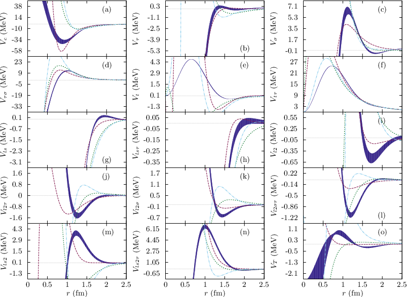
In Figs. 7 and 8 we show the OPE-Gaussian potential in partial wave and operator basis respectively with the error bands propagated with the corresponding correlation matrix from the fit to the experimental data. As we see, these error bands are smaller than the discrepancy with Reid93 [15] NijmII [15] and AV18 [16]. This may be a hint that systematic errors induced by the bias involved in the choice of the several potentials, as first noted in Ref. [22, 23, 24], may indeed play a relevant role in the total evaluation of nuclear uncertainties.
In Fig. 9 we present the lowest np and pp phase shifts and their errors based on the OPE-Gaussian potential and compared with the Reid93 [15], NijmII [15] and AV18 [16] potential phases. In Tables 8 , 9 and 10 the low angular momentum phases as a function of the LAB energy with their errors propagated from the fit are listed.
The resulting Wolfenstein parameters, Eq. (1), for the OPE-Gaussian potential are depicted in Figs. 10, 11, 12 and 13 for LAB energies and MeV respectively with their corresponding errors. For comparison we also show the same quantities calculated with the 1993-high quality Reid93 [15], NijmII [15] and AV18 [16] potentials.


V Conclusions and outlook
We summarize our main points. The determination of uncertainties in theoretical nuclear physics is one of the most urgent issues to be solved in order to establish the predictive power of ab initio nuclear structure calculations. One certain source for these uncertainties is the errors of the phenomenological NN interaction stemming from the finite accuracy of experimental scattering data as well as local scarcity in certain regions of the plane and an abundance bias in some other regions. Any statistical analysis of this sort assumes a model both for the signal and the noise which can only be checked a posteriori. In order to carry out such an analysis the lack of bias in the data and the model has to be established with a given confidence level. If normal errors on the data are assumed, the check can be made by applying normality tests to the residuals between the fitted model and the experimental data. We have used some classical tests and the highly demanding recently proposed Tail-sensitive Quantile-quantile test with a confidence level of . Based on the outcome there is no serious reason to doubt on the normality of residuals of the self-consistent database obtained in our PWA of np and pp scattering data below pion production threshold.
We remind that this normality test actually checks for the assumption, underlying any least squares fit, that the data themselves follow a normal distribution. With this fixed database one can then look for different representations of the potential which facilitate a straightforward implementation in any of the many available powerful methods which are currently available for solving the multi-nucleon problem.
We provide a user friendly potential which consists of a short range local part with 21-operators multiplying a linear superposition of Gaussian functions. The resulting fitted potential passes the normality tests satisfactorily and hence can be used to estimate statistical uncertainties stemming from NN scattering data.
Our findings here seem to confirm a previous study of us when we compare the current OPE-Gauss potential including statistical error bands with previous potentials such as NijmII, Red93 or AV18 (without statistical bands); errors in the potential are dominated by the form of the potential, rather than by the experimental data. Nonetheless, a thorough study of these kind of errors requires repeating the present analysis with an identical database with the most general potentials and functional forms, and looking for discrepancies in the nuclear structure calculations outcome.
We thank Elías Moreno for a statistician’s point of view, Antonio Bueno for disclosing the experimentalist’s feelings and Lorenzo Luis Salcedo for an introduction to the Bayesian approach. We also thank Eduardo Garrido for numerical checks.
References
- [1] R. Machleidt, Adv.Nucl.Phys. 19, 189 (1989).
- [2] W. Glöckle, The quantum mechanical few-body problem (Springer Berlin, 1983).
- [3] L. Puzikov, R. Ryndin, and J. Smorodinsky, Nuclear Physics 3, 436 (1957).
- [4] M. J. Evans and J. S. Rosenthal, Probability and statistics: The science of uncertainty (Macmillan, 2004).
- [5] W. T. Eadie and F. James, Statistical methods in experimental physics (World Scientific, 2006).
- [6] T. Editors, Phys. Rev. A 83, 040001 (2011), URL http://link.aps.org/doi/10.1103/PhysRevA.83.040001.
- [7] H. Stapp, T. Ypsilantis, and N. Metropolis, Phys.Rev. 105, 302 (1957).
- [8] R. Arndt and M. Macgregor, Methods in Computational Physics 6, 253 (1966).
- [9] J. Perring, Nuclear Physics 42, 306 (1963).
- [10] R. A. Arndt and M. H. MacGregor, Physical Review 141, 873 (1966).
- [11] M. H. MacGregor, R. A. Arndt, and R. M. Wright, Phys.Rev. 169, 1128 (1968).
- [12] R. Arndt and L. Roper, Nucl.Phys. B50, 285 (1972).
- [13] J. Bergervoet, P. van Campen, W. van der Sanden, and J. J. de Swart, Phys.Rev. C38, 15 (1988).
- [14] V. G. Stoks, R. Timmermans, and J. de Swart, Phys.Rev. C47, 512 (1993a), eprint nucl-th/9211007.
- [15] V. G. J. Stoks, R. A. M. Klomp, C. P. F. Terheggen, and J. J. de Swart, Phys. Rev. C49, 2950 (1994), eprint nucl-th/9406039.
- [16] R. B. Wiringa, V. Stoks, and R. Schiavilla, Phys.Rev. C51, 38 (1995), eprint nucl-th/9408016.
- [17] R. Machleidt, Phys.Rev. C63, 024001 (2001), eprint nucl-th/0006014.
- [18] F. Gross and A. Stadler, Phys.Rev. C78, 014005 (2008), eprint 0802.1552.
- [19] R. Navarro Perez, J. Amaro, and E. Ruiz Arriola (2012a), eprint 1202.2689.
- [20] R. Navarro Perez, J. Amaro, and E. Ruiz Arriola, PoS CD12, 104 (2013a), eprint 1301.6949.
- [21] K. Chadan and P. C. Sabatier, Inverse problems in quantum scattering theory (Springer Publishing Company, Incorporated, 2011).
- [22] R. Navarro Perez, J. Amaro, and E. Ruiz Arriola (2012b), eprint 1202.6624.
- [23] R. Navarro Perez, J. Amaro, and E. Ruiz Arriola, PoS QNP2012, 145 (2012c), eprint 1206.3508.
- [24] J. Amaro, R. N. Perez, and E. R. Arriola (2013), eprint 1310.7456.
- [25] J. Toivanen, J. Dobaczewski, M. Kortelainen, and K. Mizuyama, Phys.Rev. C78, 034306 (2008), eprint 0806.1914.
- [26] J. Dudek, B. Szpak, B. Fornal, and A. Dromard, Physica Scripta 2013, 014002 (2013).
- [27] J. Dobaczewski, W. Nazarewicz, and P. G. Reinhard (2014), eprint 1402.4657.
- [28] A. Saltelli and S. Funtowicz, Issues in Science and Technology, Fall 2013, 79 (2013).
- [29] J. B. Aviles, Phys. Rev. C6, 1467 (1972).
- [30] R. Navarro Perez, J. Amaro, and E. Ruiz Arriola, Prog.Part.Nucl.Phys. 67, 359 (2012d), eprint 1111.4328.
- [31] S. Aldor-Noiman, L. D. Brown, A. Buja, W. Rolke, and R. A. Stine, Amer. Statist. 67, 249 (2013).
- [32] E. Matsinos, Phys.Rev. C56, 3014 (1997).
- [33] R. Navarro Perez, J. Amaro, and E. R. Arriola (2013b), eprint 1310.8167.
- [34] I. BIPM, I. IFCC, and I. IUPAC, Oiml 2008 evaluation of measurement data—guide to the expression of uncertainty in measurement (1995).
- [35] R. T. Birge, Physical Review 40, 207 (1932).
- [36] R. N. Kacker, A. Forbes, R. Kessel, and K.-D. Sommer, Metrologia 45, 257 (2008).
- [37] R. A. Arndt, L. D. Roper, R. A. Bryan, R. B. Clark, B. J. VerWest, et al., Phys.Rev. D28, 97 (1983).
- [38] R. Navarro Perez, J. Amaro, and E. R. Arriola, Phys.Rev. C88, 024002 (2013c), eprint 1304.0895.
- [39] R. Navarro Perez, J. Amaro, and E. R. Arriola, Phys.Rev. C88, 064002 (2013d), eprint 1310.2536.
- [40] W. H. Press, Numerical recipes 3rd edition: The art of scientific computing (Cambridge university press, 2007).
- [41] V. Stoks, R. Kompl, M. Rentmeester, and J. de Swart, Phys.Rev. C48, 792 (1993b).
- [42] J. Beringer et al. (Particle Data Group), Phys.Rev. D86, 010001 (2012).
- [43] O. Behnke, K. Kröninger, G. Schott, and T. Schörner-Sadenius, Data Analysis in High Energy Physics: A Practical Guide to Statistical Methods (John Wiley & Sons, 2013).
- [44] W. Conover, Practical nonparametric statistics (John Wiley, 1980).
- [45] A. N. Kolmogorov, Giornale dell Istituto Italiano degli Attuari 4, 83 (1933).
- [46] N. Smirnov, Ann. Math. Statist. 19, 279 (1948).
- [47] R. Von Mises, Mathematical theory of probability and statistics (Academic Press, 1964).
- [48] R. N. Perez, J. Amaro, and E. R. Arriola, Phys.Rev. C89, 024004 (2014), eprint 1310.6972.
- [49] M. Srivastava and D. W. Sprung, in Advances in Nuclear Physics (Springer, 1975), pp. 121–218.
- [50] S. Aoki, T. Hatsuda, and N. Ishii, Prog.Theor.Phys. 123, 89 (2010), eprint 0909.5585.
- [51] S. Aoki (Sinya AOKI for HAL QCD Collaboration), Prog.Part.Nucl.Phys. 66, 687 (2011), eprint 1107.1284.
- [52] S. Aoki, Eur.Phys.J. A49, 81 (2013), eprint 1309.4150.
- [53] N. Ishii et al. (HAL QCD Collaboration), Phys.Lett. B712, 437 (2012), eprint 1203.3642.
- [54] A. Walker-Loud (2014), eprint 1401.8259.
- [55] C. V. D. Leun and C. Alderliesten, Nucl. Phys. A380, 261 (1982).
- [56] I. Borbély, W. Grüebler, V. König, P. A. Schmelzbach, and A. M. Mukhamedzhanov, Phys. Lett. 160B, 17 (1985).
- [57] N. L. Rodning and L. D. Knutson, Phys. Rev. C41, 898 (1990).
- [58] S. Klarsfeld, J. Martorell, J. A. Oteo, M. Nishimura, and D. W. L. Sprung, Nucl. Phys. A456, 373 (1986).
- [59] D. M. Bishop and L. M. Cheung, Phys. Rev. A20, 381 (1979).
- [60] J. J. de Swart, C. P. F. Terheggen, and V. G. J. Stoks (1995), eprint nucl-th/9509032.