Replica exchange molecular dynamics optimization of tensor network states for quantum many-body systems
Abstract
The tensor network states (TNS) methods combined with Monte Carlo (MC) techniques have been proved a powerful algorithm for simulating quantum many-body systems. However, because the ground state energy is a highly non-linear function of the tensors, it is easy to get stuck in local minima when optimizing the TNS of the simulated physical systems. To overcome this difficulty, we introduce a replica-exchange molecular dynamics optimization algorithm to obtain the TNS ground state, based on the MC sampling techniques, by mapping the energy function of the TNS to that of a classical dynamical system. The method is expected to effectively avoid local minima. We make benchmark tests on a 1D Hubbard model based on matrix product states (MPS) and a Heisenberg - model on square lattice based on string bond states (SBS). The results show that the optimization method is robust and efficient compared to the existing results.
pacs
71.10.-w, 75.10.Jm, 03.67.-a, 02.70.-cAugust 24, 2026
I Introduction
Developing efficient methods to simulate strongly correlated quantum many-body systems is one of the central tasks in modern condensed matter physics. Recently developed tensor network states (TNS) methods, including the matrix product states (MPS), [1, 2, 3] and the projected entangled pair states (PEPS), [4] string bond states(SBS) [5], multi-scale entanglement renormalization ansatz (MERA) [6]etc. provide a promising scheme to solve the long standing quantum many-body problems. In this scheme the variational space can be represented by polynomially scaled parameters, instead of exponential ones. Once we have the TNS representation of the many-particle wave functions, the ground state energies as well as corresponding wave functions can be obtained variationally. However, in practice it is still a great challenge to obtain the ground state of some complicate physical systems (such as, frustrated systems and fermionic systems in two dimension) in the TNS scheme.
Several difficulties reduce the efficiency. First, though the polynomial scaling, the computational cost respect to the virtual dimension cut-off is still very high, particularly, in two and higher dimensions. For example, the scaling is for periodic MPS algorithm,[7] for the PEPS algorithm[8]. For many important systems, in particular, the fermionic systems, the parameter should be rather large to capture the key physics. However, limited by current computation ability, we can only deal with small , typically less than 10. To overcome this difficulty, in seminal works, Sandvik et. al[9] (based on MPS) and Schuch et. al. [5] (based on SBS) introduced a Monte Carlo (MC) sampling technique instead of contraction to reduce the computational cost. The technique has soon been applied to more general TNS, such as PEPS. [10] Based on the MC sampling technique, the MPS scaling can be reduced from to for periodic boundary condition (PBC). [9] For SBS,[5] the scaling is O() for a 2D open boundary condition (OBC) system and O() for a 2D periodic system with MC sampling technique, which is significantly lower than the standard contraction methods. For more general PEPS case, the scaling can also be well reduced. [10]
Secondly, the energy function is a highly non-linear function of the tensors. With the increasing of , the parameter space will be very large and it is very easy to be trapped in some local minima, when minimizing the energies, especially for complicated or frustrated systems with a large number of low energy excitations. Here, we focus on overcoming this difficulty.
In this work, we develop an efficient algorithm to obtain the ground state energy as well as wave function of a TNS based on the MC sampling method. We map the quantum many-particle problem to a classical mechanical problem, in which we treat the tensor elements as the generalized coordinates of the system. We optimize the energy of the system using a replica exchange molecular dynamics method.[11, 12] By exchanging the system configurations among higher and lower temperatures, it can explore large phase space and therefore effectively avoid being stuck in the local minima. The replica exchange method has been proved very successful in treating classical spin glass [13] and frustrated spin systems[14] which also suffer from the local minima problem. It also has been successfully used to optimize other highly non-linear problems, such as three-tangle of general mixed states. [15] Here, we introduce this method in the TNS scheme for the quantum many-body systems. We make benchmark tests of the method for a 1D Hubbard model [16] using MPS and the 2D - Heisenberg model using SBS. [17] The results show that this method is efficient and robust. It is also worth to emphasize that the method introduced here is not limited to the special type of TNS, but applies to general TNS.[10]
II Methods
For simplicity, we describe our method using the example of MPS type of wave functions. The method can be easily generalized to other types of TNS, e.g., SBS [5] and PEPS. [10] The many-particle wave functions of one dimensional periodic systems with sites, can be written in the MPS[3], i.e.,
| (1) |
where, is the dimension of the physical indices , and for fixed physical index , are matrices on site , where is the Schmidt cut-off. Given a Hamiltonian for a system, the total energy of this system is a function of the tensors at each lattice site , i.e., . The main task is to find the ground state wave function and its energy, that is, to find the global minimum of the function and the corresponding value of . This problem can be mapped to optimizing the total energy of a classical mechanical system, in which the elements of the tensor are treated as the generalized coordinates of the system. We introduce the Lagrangian of the artificial system,
| (2) |
where is the artificial mass of the “particles”, and we use =1 in all the simulations. is the velocity of corresponding matrix defined on each lattice site. The norm of matrix is defined as
| (3) |
where is the velocity corresponding to which is the elements of .
We therefore have the Euler-Lagrange equation (we drop the site index for simplicity),
| (4) |
which leads to,
| (5) |
The energy and its derivative respect to given can be easily calculated by MC sampling the physical configuration space. [9, 5] Since the MC sampling method for TNS has been described in details in Refs. [9, 5], we shall not repeat it here.
Equation (5) can be solved via the molecular dynamics (MD) method, [18] using a velocity Verlet’s algorithm,
| (6) |
where,
| (7) |
and,
| (8) |
Now we introduce a temperature for each tensor as the average “kinetic” energies of the “particles”, i.e.,
| (9) |
where is the total degree freedoms (number of “particles”) of tensor . [19] When the temperature approaches zero, both and also approach zero, we then obtain the minimum of , i.e., the ground state energy of the quantum system, and corresponding wave function. When temperature is sufficiently low, the system can be approximated as harmonic oscillations around their equilibrium positions, and therefore, according to the classical statistics the total energy of the system is .
We can run the MD simulation at a given temperature through exchanging energies with a heat bath. Since we are not interested in the real “dynamics” of the system, one can use the simplest velocity rescaling thermostat: in order to fix the temperature at , we rescale the velocity by a factor at each MD step, where is the instantaneous temperature defined in Eq. (9). Note that when scaling a tensor to , the energy of the system remains unchanged. Therefore, we normalize the tensors by dividing them the largest absolute value of the elements of each tensor after each MD step, to keep the temperature well defined. Furthermore, any change of the tensor that is parallel to during the MD steps have no contribution to the energy. To improve the efficiency, we orthogonalize the velocity to at each MD step before we rescaling the velocity to the given temperature,
| (10) |
where the inner product of two matrices is defined as,
| (11) |
Usually the ground state energy of a simple system can be obtained by a simulated annealing method, i.e., one starts from a high temperature of the system, and gradually decreases the temperature to zero. If the temperature cooling is sufficiently slow, in principle one should get the global minimum of the system. However, since the energy is highly non-linear function of the tensors, and for frustrated physical models, which have many metastable states, in practice, it often easily be trapped in some local minima.
Here, we adopt the replica exchange (also known as parallel tempering) [11, 12] MD method, which simulates replicas simultaneously, and each at a different temperature covering a range of interest, to avoid being stuck in local minima. Each replica runs independently, except after certain steps the configuration can be exchanged between neighboring temperatures, according to the Metropolis criterion,
| (12) |
where in which and are the average energies of the th and the -th replica in a range of certain MD steps. The inclusion of high- configurations ensures that the lower temperature systems can access a broader phase space and avoid being trapped in local minima. During the simulation, we keep the highest temperature and lowest temperature fixed, whereas the rest temperatures distribute exponentially between the highest and lowest temperatures at the start of simulation. During the simulation, the temperatures (except and ) are adjusted to ensure that the exchange rates between the replica are roughly equal.[15]
The lower the minimal temperature , the more accurate the results one can obtain. In principle, has to approach zero to get the real ground state. However, decrease the will increase the computational cost (the number of replica temperatures). Instead, one could continue to lower the temperature sequentially to a desired low temperature, or adopt a local minimizer (e.g., conjugate gradient method) after we finish the replica exchange MD simulations, to get more accurate ground state.
It is worth noting that a direct use of Monte Carlo method instead of MD to update the tensors themselves (i.e., one directly change the tensor elements according to the Metropolis criterion for the total energy) are not applicable for the scheme. The reason is that the energy obtained from MC sampling is not bounded from below. Therefore, it is very easy to be trapped in a false energy minimum (i.e., the energy minimum due to inadequate MC sampling, which may be much lower than the real energy of the system), especially if the sampling is not large enough, if a Monte Carlo updating method is used. In contrast, the MD method does not suffer from this problem.
III Results and discussion
In this section, we present the benchmark tests of our scheme on one-dimensional (1D) Hubbard model and two-dimensional (2D) - model. Since 1D model has been well studied and has many efficient schemes, we simply present the results without detailed discussion. We discuss more detailed features of the scheme for the 2D model.
III.1 One-dimensional Hubbard model
To test our scheme, we compute the ground state energy of the 1D Hubbard model,[20]
| (13) |
To simulate the 1D Hubbard model, we first transform it to a spin model via Jodran-Wigner transformation. The many-particle wave function of the ground state of the corresponding spin model is presented by a MPS. We optimize the energy using the replica exchange MD method described in the method section. We use 48 temperatures, with the highest temperature =10-3, and lowest temperature =10-7. The MD time step =0.5. During the replica exchange MD, we use 3000 MC (each spin flip is considered a MC sampling) samplings per MD step, where is the length of the Hubbard chain. We further cool down the temperature sequentially to 10-12 to get more accurate ground state energy, after the replica exchange MD simulation. The number of MC sampling to calculate the final total energy is 50000.
We compare our results to those obtained from the exact diagonalization method in Table 1, for a =14 sites, half-filling Fermion Hubbard model, with PBC, for various parameters. We take Schmidt cut-off =6 - 14 for the MPS. As one can see from the table, we have obtained high accurate results using the replica-exchange MD optimization method, compared with those obtained from exact diagonalization method.
| D | U=0.1 | U=1 | U=3 | U=10 |
|---|---|---|---|---|
| 4 | -1.25074 | -1.04271 | -0.68991 | -0.26691 |
| 6 | -1.25728 | -1.04922 | -0.69508 | -0.26845 |
| 8 | -1.25880 | -1.05059 | -0.69608 | -0.26873 |
| 10 | -1.25903 | -1.05092 | -0.69627 | -0.26875 |
| 12 | -1.25912 | -1.05100 | -0.69632 | -0.26876 |
| 14 | -1.25914 | -1.05104 | -0.69633 | -0.26876 |
| Exact | -1.25916 | -1.05105 | -0.69634 | -0.26878 |
III.2 Two-dimensional - model
We simulate the typical two dimensional frustrated spin- Heisenberg model, namely the - model on a square lattice. The Hamiltonian of the model is,
| (14) |
The spin operators obey =3/4, whereas and denote the nearest and next-nearest neighbor spin pairs, respectively, on the square lattice. - model has became a promising candidate model whose ground state may be a spin liquid state near .[21, 22, 23]
Two kinds of generalization to higher dimensions of MPS, i.e., PEPS and SBS can be used to simulate two dimensional systems. PEPS has extremely high scaling with the tensor dimension truncation , which are , for OBC and PBC respectively.[17] In contrast, SBS has much lower scaling to , which are and for OBC and PBC respectively. Here, as a benchmark, we demonstrate our scheme using the SBS type of wave functions.
The wave functions represented in SBS form can be written as,
| (15) |
where is a certain string pattern which contains a set of strings . The product of matrices with bond dimension over means over the sites in the order in which appear in the string . In this work, we use two patterns of the SBS, i.e., the long strings and small loops as shown in Fig. 1. The two types of SBS satisfy both area law [5] and size-consistency. [24]
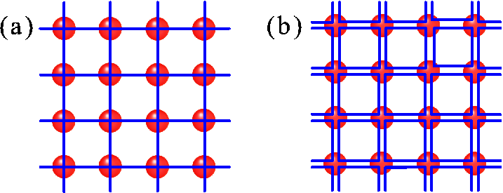
In our simulations, we use =96 temperatures. Initially, the temperatures distribute exponentially between the highest () and lowest () temperatures. For each temperature, we start from random tensors. During the simulations, we adjust the temperatures after configuration exchange for 10 times, whereas there are 300 MD steps between the two configuration exchanges, with a step length =0.01. When sampling the spin configurations, we enforce =0. For each MD step, we sample about 10000 spin configurations. The energies used for temperature exchange are averaged over 300 MD steps. We find that adding some small random velocities every 3000 MD steps to the system can significantly accelerate the convergence, especially for the large physical systems. After we finish the replica-exchange MD optimization, we further decrease the temperature to obtain more accurate results.

We simulate the model for [0, 1], on square lattices, with both OBC and PBC. To illustrate how the algorithm works, we show in Fig. 2(a), how the energies evolve during the MD processes at temperature =, , , and for a 66 OBC system with =0.7. We use with =8 for the long strings, and =4 for the loops. Note that the exact values of the temperatures may change during the process. As expected, the energies of each temperature decreases quickly first to the “equilibrium” energy, and then fluctuate around it. Especially, the energy of the lowest temperature decreases quickly to the energy that near the ground state energy. The energy of the system at higher temperatures fluctuate more dramatically than those at lower temperatures, because the systems have larger “kinetic” energy. By the temperature exchange, it may help the system from being stuck in some local minima.
Figure 2(b) depicts the total energies as functions of temperatures after 5, 30, 50, 150, 250 times of temperature exchanges for the above system. As we see that the energies at lower temperatures quickly decrease to near the ground state energy. After enough MD and temperature exchanges, the energy-temperature curves become stable. In this situation, we expect that we have obtained reliable ground state. We then further decrease the temperature to get more accurate ground state energy.


The improvement of energy by increasing the virtual dimension cut-off and adding new SBS patterns are shown in Fig. 3 for a 1010 OBC lattice, with =0, 0.5 and 1.0. First, we use only the long strings. We find that =8 (S8) has converged the results. We then add the pattern of small loops, and the energies improve significantly. We find =6 (S8L6) for the loops converge the results. As one can see that the energy obtained by SBS is still about 1 - 3% higher than the exact results or those obtained from PEPS. This error is from the limitation of the SBS wave functions, and is not from the optimization process. [5, 17] Unlike PEPS, the quality of SBS cannot be improved by simply increasing the dimension of the tensors alone. However, one can systematically improve the SBS by adding more patterns of the tensor strings. [5] Fortunately, the computational cost increases only linearly with the number of string patterns, in contrast to the extremely high scaling with the tensor dimension in the PEPS method. It is very valuable to study how to improve the SBS wave functions by adding new types of string patterns. We leave this for future study.
We then compare the obtained results using the method described in the paper with the results obtained from exact diagonalization method or PEPS method, and those in Ref. 17 which also used SBS on lattices of size 44, 66 and 1010 with both OBC and PBC. It can be seen that in all cases the ground state energies optimized by replica-MD method are improved from the ones obtained using the original optimization method. For some points, especially in the strong frustration region, the improvement is significant.
It is worth pointing out that the MD optimization scheme developed in this work can apply not only to the MPS and SBS types of TNS, but also to more general TNS, e.g., PEPS with some modification. [10] It is suitable to study the systems with rough energy surface, where other optimization methods may fail. The current method with MC sampling has other advantages, e.g., it is easy to implement the constrains in physical space. For example, it is easy to simulate the system in canonical ensemble using this method, with particle number conservation, as well as the grand canonical ensemble with fixed chemical potential, whereas it is difficult to enforce particle number conservation in the contraction methods.
IV Summary
The tensor network states method has been proved a powerful algorithm for simulating quantum many-body systems. However, because the ground state energy is a highly non-linear function of the tensors, it is easy to be trapped in the local minima when optimizing the TNS of the simulated physical systems. We have introduced a replica exchange molecular dynamics method to optimize the tensor network states. We demonstrate the method on a one dimensional Hubbard model based on MPS and the two dimensional frustrated Heisenberg - model on square lattices based on SBS. For the one dimensional model, our results are in excellent agreement with the those from exact diagonalization method. For the two dimensional model, our results show improvement over the existing calculations, especially in the strong frustrated region. The results demonstrate that our method is efficient and robust. The method can be generalized to other forms of TNS, e.g. PEPS with some modification, and provides a useful tool to investigate complicate many-particle systems, such as frustrated systems and fermionic systems.
Acknowledgements.
LH acknowledges the support from the Chinese National Fundamental Research Program 2011CB921200, the National Natural Science Funds for Distinguished Young Scholars and NSFC11374275. YH acknowledges the support from the Central Universities WK2470000004, WK2470000006, WJ2470000007 and NSFC11105135.References
- [1] G. Vidal, Phys. Rev. Lett. 91, 147902 (2003).
- [2] G. Vidal, Phys. Rev. Lett. 93, 040502 (2004).
- [3] M. Fannes, B. Nachtergaele, and R. Werner, Communications in Mathematical Physics 144, 443 (1992).
- [4] F. Verstraete and J. I. Cirac, cond-mat/0407066 (2004).
- [5] N. Schuch, M. M. Wolf, F. Verstraete, and J. I. Cirac, Phys. Rev. Lett. 100, 040501 (2008).
- [6] G. Vidal, Phys. Rev. Lett. 99, 220405 (2007).
- [7] F. Verstraete, D. Porras, and J. I. Cirac, Phys. Rev. Lett. 93, 227205 (2004).
- [8] V. Murg, F. Verstraete, and J. I. Cirac, Phys. Rev. A 75, 033605 (2007).
- [9] A. W. Sandvik and G. Vidal, Phys. Rev. Lett. 99, 220602 (2007).
- [10] L. Wang, I. Pižorn, and F. Verstraete, Phys. Rev. B 83, 134421 (2011).
- [11] R. H. Swendsen and J.-S. Wang, Phys. Rev. Lett. 57, 2607 (1986).
- [12] C. J. Geyer, Computer Science and Statistics, Proceedings of the 23rd Symposium on the interface (Interface Foundation, 1991).
- [13] E. Marinari, G. Parisi, and J. J. Ruiz-Lorenzo, Phys. Rev. B 58, 14852 (1998).
- [14] K. Cao, G.-C. Guo, D. Vanderbilt, and L. He, Phys. Rev. Lett. 103, 257201 (2009).
- [15] K. Cao, Z.-W. Zhou, G.-C. Guo, and L. He, Phys. Rev. A 81, 034302 (2010).
- [16] M. P. A. Fisher, P. B. Weichman, G. Grinstein, and D. S. Fisher, Phys. Rev. B 40, 546 (1989).
- [17] A. Sfondrini, J. Cerrillo, N. Schuch, and J. I. Cirac, Phys. Rev. B 81, 214426 (2010).
- [18] J. M. Haile, Molecular Dynamics Simulation: Elementary Methods (Wiley, 1997).
- [19] Alternatively, one can define a temperature for the whole system in a similar way.
- [20] H. Frahm, F. Göhmann, A. Klümper, and K. V. E., The One-Dimensional Hubbard Model (Cambridge University Press, 2005).
- [21] L. Wang, Z.-C. Gu, F. Verstraete, and X.-G. Wen, cond-mat/1112.3331 (2012).
- [22] L. Wang, D. Poilblanc, Z.-C. Gu, X.-G. Wen, and F. Verstraete, Phys. Rev. Lett. 111, 037202 (2013a).
- [23] H.-C. Jiang, H. Yao, and L. Balents, Phys. Rev. B 86, 024424 (2012).
- [24] Z. Wang, Y. Han, G.-C. Guo, and L. He, Phys. Rev. B 88, 121105(R) (2013b).
- [25] H. Schulz, T. Ziman, and D. Poilblanc, cond-mat/9402061 (1994).