Cloud-Based Optimization: A Quasi-Decentralized Approach to Multi-Agent Coordination
Abstract
New architectures and algorithms are needed to reflect the mixture of local and global information that is available as multi-agent systems connect over the cloud. We present a novel architecture for multi-agent coordination where the cloud is assumed to be able to gather information from all agents, perform centralized computations, and disseminate the results in an intermittent manner. This architecture is used to solve a multi-agent optimization problem in which each agent has a local objective function unknown to the other agents and in which the agents are collectively subject to global inequality constraints. Leveraging the cloud, a dual problem is formulated and solved by finding a saddle point of the associated Lagrangian.
I Introduction
Distributed optimization and algorithms have received significant attention during the last decade, e.g., [1, 20, 10, 8, 15, 22, 6], due to the emergence of a number of application domains in which individual decision makers have to collectively arrive at a decision in a distributed manner. Examples of these applications include communication networks [12, 5], sensor networks [13, 23, 2], multi-robot systems [26, 21], and smart power grids [3].
Distributed algorithms are needed mainly because the scale of large distributed systems is such that no central, global decision maker can collect all relevant information, perform all required computations, and then disseminate the results back to individual nodes in the network in a timely fashion. However, one can envision a scenario in which such globally obtained information can be used in conjunction with local computations performed across the network. This could, for example, be the case when a cloud computer is available to collect information, as was envisioned in [9]. The question then becomes that of designing the appropriate architecture and algorithms that can leverage this mix of prompt decentralized computations with intermittent centralized computations.
One approach to multi-agent optimization that will prove useful towards achieving this hybrid architecture is based on primal-dual methods to find saddle points of a problem’s Lagrangian [19, 7]. In fact, the study of saddle point dynamics in optimization can be traced back to earlier results from Uzawa in [24], which will provide the starting point for the work in this paper. The primary difference between this paper and the established literature is the cloud-based architecture used to solve the problem; indeed the architecture is this paper’s main contribution. The architecture we introduce uses a cloud computer in order to receive information from each agent, perform global computations, and transmit this information to other agents. We will see that this division of labor results in globally asymptotic convergence to an -ball about a Lagrangian’s saddle point.
The goal of this paper is to serve as a first attempt at understanding how centralized, cloud-based information might be injected in an intermittent but useful manner into a network of agents where such information would otherwise be absent. In order to highlight how the cloud might prove useful to such a system, we choose to consider an extreme case where no inter-agent communication occurs at all, in contrast to existing distributed multi-agent optimization techniques, e.g., [14, 16, 17, 18]. Under this architecture the cloud handles all communications, and computations are divided between the cloud and the agents in the network.
The rest of the paper is organized as follows: Section II gives a detailed problem statement and describes the cloud architecture, and then Section III provides the convergence analysis for the given problem. Next, Section IV provides numerical results to demonstrate the viability of this approach, and finally Section V concludes the paper.
II Problem Statement and Architecture
II-A Architecture Motivation
We now explain the interplay between the cloud architecture and the problem under consideration here. A detailed explanation is given below, with a summary and example following at the end of this section. Consider a collection of agents indexed by , , where each agent is associated with a scalar state and where there is no communication at all between the agents. Let the task agent is trying to solve be encoded in a strictly convex objective functions in , . Each agent is assumed to have no knowledge of other agents’ objective function and each agent’s only goal is to minimize its own objective function.
To that end, agent is assumed to have immediate access to its own state, which seemingly makes this problem very simple. However, what prevents agent from simply computing and setting this equal to zero – a completely decentralized operation as only depends on – is that the agents need to coordinate their actions through a globally defined constraint, that can, for example, represent finite resources that must be shared across the team. In this paper it is assumed that agent cannot measure the state of any other agents and, as mentioned above, that there is no communication between agents. Instead, this information must be obtained in some other manner, which is where the cloud will enter into the picture.
The team-wide coordination is encoded through the global constraint
| (1) |
where is a state vector containing the states of all agents in the network. It is further assumed that each is convex. The cloud architecture discussed here applies to any problem in which the user has selected functions and that meet the above criteria and the forthcoming analysis fully characterizes all such problem formulations.
Let
| (2) |
Then is strictly convex and the problem under consideration becomes that of minimizing subject to . The Kuhn-Tucker Theorem on concave programming (e.g., [25]) states that the optimum of this constrained problem is a saddle point of the Lagrangian
| (3) |
where the Kuhn-Tucker (KT) multipliers satisfy for all . We assume that the minimizer of with respect to , denoted , is a regular point of so that there is a unique saddle point, , of [4]. Using that is convex in and concave in , the saddle point can be shown to satisfy the inequalities
| (4) |
for all admissible and .
Using Uzawa’s algorithm [24], the problem of finding can be solved from the initial point using the difference equations
| (5) |
| (6) |
where is a constant, and where the maximum defining is taken component-wise so that each component of is projected onto the non-negative orthant of , denoted by . In the context of Uzawa’s algorithm, the element of the state vector is updated according to
| (7) |
Under the envisioned organization of the agents and the lack of inter-agent communication, Uzawa’s algorithm cannot be directly applied. To see this, observe that if agent is to compute its own state update using Equation (7), a fundamental problem is encountered: computing will require knowledge of states of (possibly all) other agents and agent cannot directly access this information. Furthermore, determining at each timestep using (6) will also require the full state vector , which no single agent has direct access to.
To account for the need of each agent for global information in applying Equation (7) and to compute using aggregated global information, the cloud computer is used. The cloud computer is taken to be capable of large batch computations and receives periodic transmissions from each agent containing each agent’s own state. The cloud computer uses the agents’ states to compute the next value of using Equation (6) and then transmits the states it received and the newly computed vector to each agent. Each agent then uses the information from the cloud to update its own state in the vein of (7).
II-B Formal Architecture Description
We first describe the actions taken to initialize the system and then explain its operation. Let the agents each be programmed with their objective functions onboard and let them either be programmed with an initial state or else be able to sense it (e.g., if it corresponds to some physical quantity). The agents are assumed to be identifiable according to their indices in so that the cloud knows the source of each transmission it receives. Each agent stores and manipulates a state vector onboard and we denote the state vector stored onboard agent by ; agent ’s copy of its own state is denoted and when we are referring to a specific point in time, say timestep , we denote agent ’s copy of its own state at this time by . The vector of KT multipliers stored onboard agent at time is denoted , though we emphasize that agent does not compute any KT vectors but instead relies on the cloud for these computations.
Before the optimization process begins, let agent send its initial state, , to the cloud and let the cloud store these states in the vector , with the superscript ’c’ denoting “cloud” and the timestep reflecting that this is the initial state. In this notation, the cloud’s copy of agent ’s state at time is denoted . Similarly, we denote the KT vector stored in the cloud at time by . Let the cloud be programmed by the user with the constraint functions, . Upon receiving the each agent’s state, the cloud symbolically computes and sends this function to agent along with some initial KT multiplier vector, , a stepsize , and the vector defined as
| (8) |
This vector contains states stored by the cloud in the vector and contains information originally from time (though in Equation (8) explicit timesteps are intentionally omitted). The subscripts in (8) denote that agent does not receive its own old state value from the cloud, which is logical since agent always knows its own most recent state. In , then, the cloud sends to agent the most recent state information it has about each other agent. In this notation, agent ’s state in is denoted . In the forthcoming analysis, always refers to the most recent state information that agent has received from the cloud and it will not be written as an explicit function of any time step. Similarly, the notation refers to the most recent KT vector sent to agent and will be written without an explicit timestep. We use the notation to denote the most recent transmission to agent containing both and .
After receiving for this first time, all agents and the cloud have the same information onboard, and each agent begins the optimization process. At timestep , each agent takes one gradient step to update its own state according to Equation (7). Simultaneously, and also at timestep , the cloud takes one gradient step to update the KT multipliers in the cloud according to Equation (6). Then at timestep , agent sends its state, , to the cloud. These transmissions are received at timestep . In timestep , the cloud sends and to agent . These vectors are received in timestep at which point the cloud updates as before and each agent takes a step to update its own state as before, thus repeating this cycle of communication and computation. It is important to note that communications cycles do not overlap and that the agents do not send their states to the cloud at every timestep, but instead do so every timestep. In addition, we emphasize that each agent’s objective function is assumed to be private throughout this process.
Due to the communications structure of the system, it is often the case that , namely that agents and will have different values for agent ’s state beacuse agent must wait to received agent ’s state from the cloud. Due these differences, Equation (5) is modified to reflect that each agent stores and manipulates a local copy of the problem. The global system therefore contains copies of the system in Equations (5) and (6) and the state vector of agent at time , , is assumed to be different from that of agent at time , , when .
Using the fact that agent will only update its state in timesteps just after it receives an update from the cloud, Equation (5) is modified so that onboard agent it is
| received at time | (9a) | ||||
| else, | (9b) |
where we define
| (10) |
Here, is defined as a vector onboard agent which contains and the most recent state of agent inserted in the appropriate place. In essence, is the most up-to-date information about all of the agents that agent has access to and contains the correct value of each other agent’s state when it is received. Note that is simply with all entries except the set to . This is because agent does not itself compute any updates for the other agents’ states which it stores onboard, but instead waits for the cloud to provide such updates.
Under the architecture of this problem, only the cloud computes values of and there is therefore only a single update equation needed for . Bearing in mind that updates to are only made in timesteps immediately after those in which the cloud receives each agent’s state, Equation (6) is modified to take the form
| (11a) | |||||
| else, | (11b) |
where denotes the projection onto and the update referred to in Equation (11a) is an update of each state’s value sent to the cloud.
We note that Equation (11b) is not indexed on a per-agent basis since only the cloud computes values of . However, we will continue to use the notation to denote the vector stored on agent at time (which may be different from the vector stored in the cloud at time ). It is important to note that the argument of is intended to reflect the time at which agent has onboard and does not imply that was computed at time or that agent computed it. In this notation represents the vector most recently sent from the cloud to agent , while represents the vector stored on agent .
With this model in mind, instead of considering the system defined in Equations (5) and (6), we consider copies of the system defined by (9b) and (11b). Using the notation that represents the vector as stored on agent at time , we can write the full update equations onboard agent as
| received at time | (12a) | ||||
| else, | (12b) |
| (13a) | |||||
| else, | (13b) |
where all changes in will result from the cloud using Equation (11b).
To illustrate the communications cycle described above, Table 1 contains a sample schedule for a single cycle. Each timestep is listed on the left and the corresponding actions taken at that timestep are listed on the right.
| Timestep | Actions |
|---|---|
| Each agent receives a transmission from the cloud and then takes step in its own copy of the problem to update (only) its own state using Equation (12a). At the same time, the cloud computes updated values using (11a). | |
| Each agent sends it state to the cloud. Equation (12b) is used by the agents and Equation (11b) is used by the cloud so that no further computations are carried out during this timestep. | |
| The cloud receives the agents’ transmissions from time and stores them in . It then sends to agent , along with , the most recently computed vector of KT multipliers (computed in timestep ). As in timestep , Equations (12b) and (11b) are used so that no further computations take place across the network. | |
| This step is identical to step . Agent receives and then takes step in its own copy of the problem to update (only) its own state using Equation (12a). At the same time, the cloud computes updated values using (11a). |
Table 1: A sample schedule for one communications cycle used by the agents and cloud to exchange information.
III Convergence Analysis
III-A Ultimate Boundedness of Solutions
In this section we will examine the evolution of the sequence
| (14) |
for an arbitrary in order to show that each agent’s local copy of the problem converges to an -ball about the point .
Specifically, the goal here is two-fold: to prove that the state of each agent’s optimization problem enters a ball of radius about the saddle point in finite time and to show that it does not leave that ball thereafter. Our approach will differ from that of [24] because we use the notion of ultimate boundedness, published after Uzawa, to simplify certain components of proof. We restate the definition of ultimate boundedness here for general discrete-time systems of the form
| (15) |
Lemma 1
Let and let be a Lyapunov candidate function for the system in Equation (15) defined on such that for all
| (16) |
for some . Let denote the closure of and let be the set
| (17) |
Let and define the set by
| (18) |
Then any solution to Equation (15) which remains in for all time and enters at some point is contained in for all time thereafter.
Proof: See [11], Theorem 5.
We also state a corollary to this result which will be used below.
Corollary 1
Proof: See [11], Corollaries 3 and 4.
Below, we will combine Lemma 1 and Corollary 1 to show that each agent’s state trajectory enters a ball of radius about , denoted , and stays within that ball. Before proving the main convergence result, we prove the following lemma which establishes a positive upper bound on the stepsizes that can be used. We will proceed in the vein of [24] and consider the Lyapunov function
| (21) |
Lemma 2
Let denote the Lagrangian in Equation (3) and set . Define the constants and by
| (22) |
and
| (23) |
where and above are (implicitly) functions of any and satisfying the conditions on pertaining to each set. Then setting
| (24) |
provides .
Proof: It suffices to show that and are both positive. The denominator of is always positive and tends to zero as so that the minimum defining does not go to zero at . The numerator of is positive by insepction and itself is therefore the square root of a positive real number.
For , we note that is convex in and concave in . The term is the negation of the directional derivative of with respect to pointing toward its minimizer, and the term is the directional derivative of with respect to pointing toward its maximizer. Both terms are therefore non-negative and because the definition of precludes , the sum of these two terms is strictly positive. The denominator in the definition of is positive as well so that itself is.
The above Lemmata and Corollaries are stated in terms of the Lagrangian defined in Equation (3). While each agent in the network stores and manipulates its own state vector and thus has its own (unique) Lagrangian, after each gradient descent step is taken and all states and KT multipliers are shared across the network, every agent ends up with the same information before taking its next step. In addition, every agent and the cloud use the same stepsize, . Then despite the distribution of information and computation throughout the network, the effective outcome of each cycle of communication and computation as described in Section II-B is one step in each of Equations (5) and (6) performed simultaneously.
Therefore, the analysis of the algorithm can be carried out for Equations (5) and (6), and for simplicity we choose to use Equations (5) and (6) in the forthcoming analysis with the understanding that it applies equally well to all agents. Due to the centrality of the convergence of Uzawa’s algorithm to this paper and in order to make use of results published after the algorithm’s original publication, we now present the main result on the ultimate boundedness of solutions to the problem at hand.
Theorem 1
Let every agent use a strictly convex objective function , and let the global constraints, , be convex with for each . Then for any stepsize such that used by all agents and the cloud, each agent’s local copy of the problem enters an -ball about in a finite number of steps and stays within that ball for all time thereafter.
Proof: In addition to using as defined in Equation (21), we equivalently use that to write
| (25) |
When it is convenient, we will also use the more concise notation .
Let gradient steps be taken at timestep so that Equation (12a) is used by all agents to update their states and Equation (11a) is used by the cloud to update . From Equation (5) we see that
| (30) |
and multiplying both sides of Equation (5) by gives
| (31) |
Using Equations (30) and (31) we see that
| (32) |
Carrying out the same steps for using Equation (6) gives
| (33) |
Summing Equations (32) and (33) gives
| (34) |
and hence
| (35) |
Suppose now that . Then using the fact that we see that
| (36) |
where the right-hand side is negative because is positive and the term inside brackets is negative. The negativity of the term in the brackets is established by observing that it is the numerator of the term defining multiplied by and, because the numerator of the fraction defining was shown to be positive, we see here that this term is negative. In fact, the term in brackets is bounded above by some negative constant, i.e., there exists such that
| (37) |
which is seen to be true because the additive inverse of this term was shown to be bounded below by a positive constant when was defined. Then for any satisfying , we see that for some .
Now suppose that . Then using Equation (35) and the fact that we see that
| (38) |
Here we see that only for and that in the set . Then the conditions of Lemma 1 are satisfied with and . In addition, for Corollary 1 we see that for any satisfying , there is some such that . Moreover, the set takes the form . Then the conditions of Corollary 1 are satisfied as well. Then enters in a finite number of steps and does not ever leave thereafter.
To summarize, a radially unbounded, discrete-time Lyapunov function was constructed. The Lyapunov function was shown to satisfy the conditions needed for ultimate boundedness and the system’s trajectory was shown to come within of the Lagrangian’s saddle point in finite time and never to be more than away thereafter.
III-B Extension to Private Optimization
While above only each agent’s objective function is assumed to be private, we can extend this problem to the case where individual states are kept private. To do this, we modify the initialization of the system. When the cloud sends to agent the function , rather than initializing agent with as a function of, e.g., , it can instead initialize agent with as a function of , where, unbeknownst to agent , , , and . By hiding the labels of each state which will be later sent to agent , these states are kept private in the sense that agent does not know which agent they belong to.
IV Simulation Results


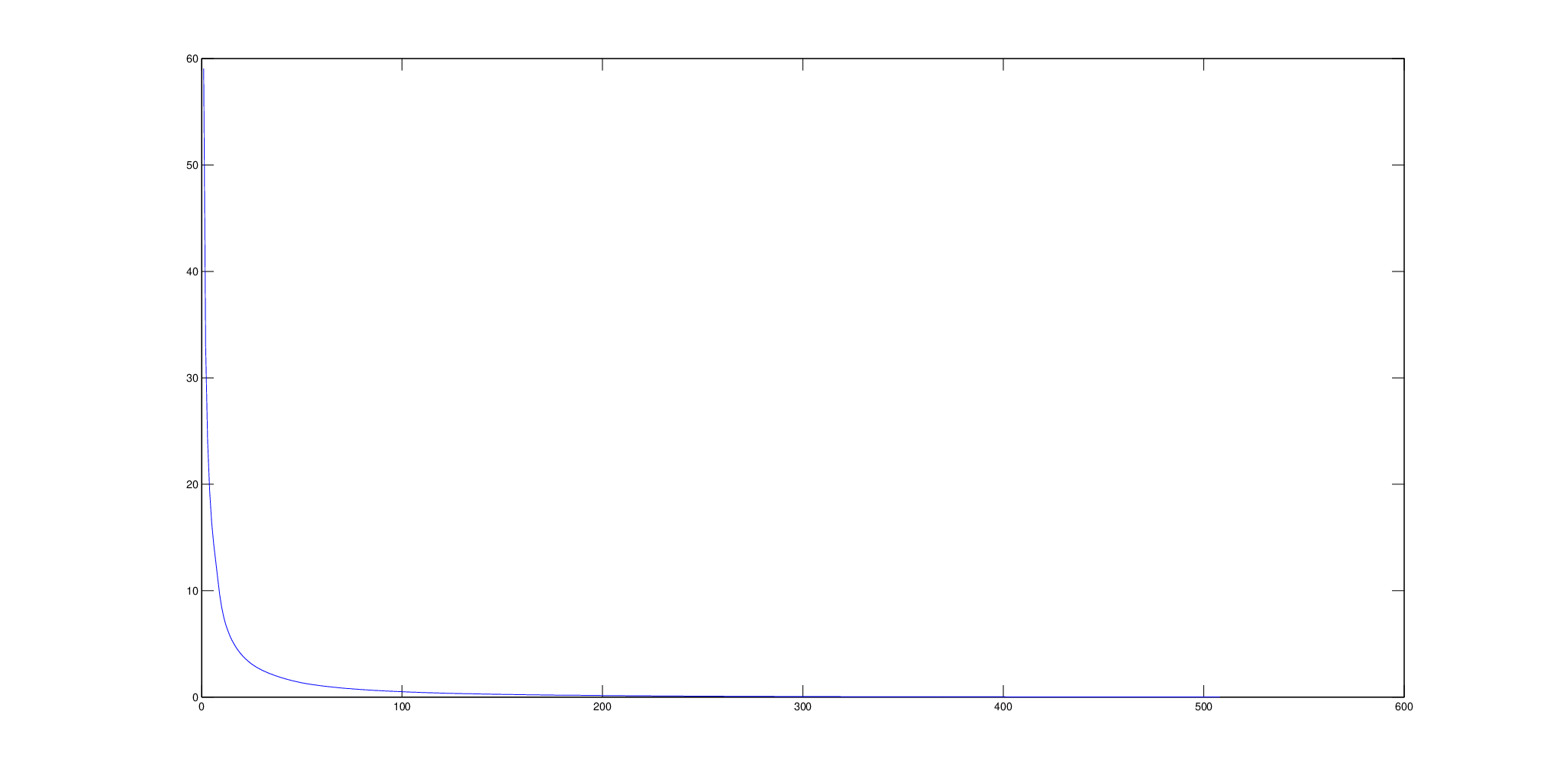
A numerical implementation of the above cloud architecture was run for a particular choice of simulation example. The problem simulated was chosen to use agents, each associated with a scalar state as above. The objective function of each agent was chosen to be , where
| (39) |
The constraints in this problem were chosen to be
| (40) |
The Lagrangian of the full problem is
| (41) |
where .
For this example, was found to be approximately and was found to be approximately . Accordingly, the stepsize used was . The gradient descent algorithm described above was initialized with all agents and the cloud having all states set to . All agents and the cloud had all Kuhn-Tucker multipliers initialized to as well. Here the value was chosen.
For the purposes of analyzing and verifying the algorithm presented here, the points and were computed ahead of time to be
| (42) |
and
| (43) |
The cloud algorithm was run for total iterations. It took iterations to enter a ball of radius about , of which were spent taking gradient descent steps and were spent communicating values across the network.
The value of was
| (44) |
and the final value of was
| (45) |
The final value of in the cloud was . Based on the definition of , this means that the square of the Euclidean distance from to is just . This result confirms both that comes within of in finite time and that it does not go more than away from after that.
To further illustrate the convergence of this problem, the histories of the states, Kuhn-Tucker multipliers, and value of over time onboard agent 1 for all timesteps are shown in Figures 1, 2, and 3, respectively. That is non-increasing in time was verified numerically in the MATLAB implementation and is evident in graph shown in Figure 3.
V Conclusion
We presented a cloud architecture for coordinating a team of mobile agents in a distributed optimization task. Each agent has direct knowledge only of its own local objective function and its own influence upon the global constraint functions but receives occasional updates from the cloud computer containing values of each other agent’s state and updated Kuhn-Tucker multipliers. Using this architecture, inequality constrained multi-agent optimization problems were proven to come within of the constrained minimum in finite time and to never be more than away thereafter. Simulation results were provided to attest to the viability of this approach.
References
- [1] Dimitri P. Bertsekas and John N. Tsitsiklis. Parallel and Distributed Computation: Numerical Methods. Prentice-Hall, Inc., Upper Saddle River, NJ, USA, 1989.
- [2] L. Carlone, V. Srivastava, F. Bullo, and G. C. Calafiore. Distributed random convex programming via constraints consensus. 52(1):629–662, 2014.
- [3] S. Caron and G. Kesidis. Incentive-based energy consumption scheduling algorithms for the smart grid. In Smart Grid Communications (SmartGridComm), 2010 First IEEE International Conference on, pages 391–396, Oct 2010.
- [4] Benoit Chachuat. Nonlinear and dynamic optimization: From theory to practice. Technical report, Automatic Control Laboratory, EPFL, Switzerland, 2007.
- [5] Mung Chiang, S.H. Low, A.R. Calderbank, and J.C. Doyle. Layering as optimization decomposition: A mathematical theory of network architectures. Proceedings of the IEEE, 95(1):255–312, Jan 2007.
- [6] Greg Droge and Magnus Egerstedt. Proportional integral distributed optimization for dynamic network topologies. In IEEE American Control Conference (ACC), 2014, June 2014.
- [7] Diego Feijer and Fernando Paganini. Stability of primal-dual gradient dynamics and applications to network optimization. Automatica, 46(12):1974–1981, December 2010.
- [8] B. Gharesifard and J. Cortes. Distributed continuous-time convex optimization on weight-balanced digraphs. Automatic Control, IEEE Transactions on, 59(3):781–786, March 2014.
- [9] Ken Goldberg and Ben Kehoe. Cloud robotics and automation: A survey of related work. Technical Report UCB/EECS-2013-5, EECS Department, University of California, Berkeley, Jan 2013.
- [10] Bruce Hendrickson and Tamara G. Kolda. Graph partitioning models for parallel computing. Parallel Comput., 26(12):1519–1534, November 2000.
- [11] James Hurt. Some stability theorems for ordinary difference equations. SIAM Journal on Numerical Analysis, 4(4):582–596, 1967.
- [12] F. Kelly, A. Maulloo, and D. Tan. Rate control in communication networks: shadow prices, proportional fairness and stability. In Journal of the Operational Research Society, volume 49, 1998.
- [13] M. Khan, G. Pandurangan, and V.S.A. Kumar. Distributed algorithms for constructing approximate minimum spanning trees in wireless sensor networks. Parallel and Distributed Systems, IEEE Transactions on, 20(1):124–139, Jan 2009.
- [14] A. Nedic and A. Ozdaglar. Distributed subgradient methods for multi-agent optimization. Automatic Control, IEEE Transactions on, 54(1):48–61, Jan 2009.
- [15] Angelia Nedic and Alex Olshevsky. Distributed optimization over time-varying directed graphs. In Decision and Control (CDC), 2013 IEEE 52nd Annual Conference on, pages 6855–6860, Dec 2013.
- [16] Angelia Nedic and Asuman Ozdaglar. On the rate of convergence of distributed subgradient methods for multi-agent optimization. In Proceedings of IEEE CDC, pages 4711–4716, 2007.
- [17] Angelia Nedić and Asuman Ozdaglar. Convergence rate for consensus with delays. Journal of Global Optimization, 47(3):437–456, 2010.
- [18] Angelia Nedic, Asuman Ozdaglar, and Pablo A Parrilo. Constrained consensus and optimization in multi-agent networks. Automatic Control, IEEE Transactions on, 55(4):922–938, 2010.
- [19] Sikandar Samar, Stephen Boyd, and Dimitry Gorinevsky. Distributed estimation via dual decomposition. In Proc. European Control Conference, pages 1511–1519, 2007.
- [20] H.D. Simon. Partitioning of unstructured problems for parallel processing. Computing Systems in Engineering, 2(2–3):135 – 148, 1991. Parallel Methods on Large-scale Structural Analysis and Physics Applications.
- [21] Daniel E Soltero, Mac Schwager, and Daniela Rus. Decentralized path planning for coverage tasks using gradient descent adaptive control. The International Journal of Robotics Research, 2013.
- [22] Andre Teixeira, Euhanna Ghadimi, Iman Shames, Henrik Sandberg, and Mikael Johansson. Optimal scaling of the admm algorithm for distributed quadratic programming. In Decision and Control (CDC), 2013 IEEE 52nd Annual Conference on, pages 6868–6873, Dec 2013.
- [23] Niki Trigoni and Bhaskar Krishnamachari. Sensor network algorithms and applications Introduction. Philosophical Transactions of the Royal Scoeity A - Mathematical, Physical, and Engineering Sciences, 370(1958, SI):5–10, JAN 13 2012.
- [24] H. Uzawa. Iterative methods in concave programming. Studies in Linear and Non-Linear Programming, 1958.
- [25] H. Uzawa. The kuhn-tucker theorem in concave programming. Studies in Linear and Non-Linear Programming, 1958.
- [26] Minyi Zhong and C.G. Cassandras. Asynchronous distributed optimization with event-driven communication. Automatic Control, IEEE Transactions on, 55(12):2735–2750, Dec 2010.