Shot-noise-limited magnetometer with sub-pT sensitivity at room temperature
Abstract
We report a photon shot-noise-limited (SNL) optical magnetometer based on amplitude modulated optical rotation using a room-temperature 85Rb vapor in a cell with anti-relaxation coating. The instrument achieves a room-temperature sensitivity of fT/ at T. Experimental scaling of noise with optical power, in agreement with theoretical predictions, confirms the SNL behaviour from T to T. The combination of best-in-class sensitivity and SNL operation makes the system a promising candidate for application of squeezed light to a state-of-the-art atomic sensor.
I Introduction
Optical magnetometers [1, 2, 3] are currently the most sensitive devices for measuring low-frequency magnetic fields and have many applications, from medical diagnostics and biomagnetism [4, 5, 6], to the detection of fields in space [7, 8], to tests of fundamental physics [9, 10, 11]. Quantum-enhanced sensitivity of optical magnetometers has been recently demonstrated using squeezing [12, 13, 14]. Quantum enhancement of a best-in-class magnetometer, i.e. of an instrument with unsurpassed sensitivity for a given parameter range, is a natural next step after these proof-of-principle demonstrations. This kind of enhancement was recently shown in gravitational wave detection, when the LIGO H1 detector was enhanced with squeezed light [15].
In this work we demonstrate a shot-noise-limited magnetometer that simultaneously is well-adapted for sensitivity enhancement with squeezed light, as in [13, 14], and has detection noise of fT at a field of T. For the given field strength and room-temperature atomic density of atoms/cm3 [16], this is among the best reported magnetometer sensitivity including those using amplitude [17, 18], frequency [19, 20] and polarization [21] modulation strategies. With two orders of magnitudes higher atomic density, a heated-cell scalar magnetometer (cell temperature 160∘ C) showed a noise level below fT in the same field range [22]. Sub-femtotesla spin-exchange-relaxation-free (SERF) magnetometers, e.g. [23, 24], are not comparable here because they operate only at near-zero field.
Our magnetometer is based on the process of nonlinear magneto-optical rotation (NMOR), also known as nonlinear Faraday rotation [25, 1]. In this process, resonant or near-resonant light produces spin coherence by optical pumping, and the spin coherence in turn produces Faraday rotation, either of the optical pumping beam itself [26], or of a separate probe beam [17], leading to a detectable signal indicating the Larmor frequency and thus the magnitude of the field. Modulation of the pumping, either in frequency (FM NMOR) [27], amplitude (AMOR) [26] or circular polarization [21] produces a resonant buildup of atomic polarization with minimal disturbance to the spin coherence. The modulation strategy significantly increases the magnetic dynamic range, i.e., the ratio between the largest detectable signal, which in NMOR can reach the geophysical field range [19, 28], and the lowest detectable signal. NMOR can give high sensitivity, due to the long ground-state coherence times, and hence narrow resonances, that arise when alkali vapours are confined with a buffer gas [29, 30] or in anti-relaxation coated cells [31, 32].
The sensitivity of optical magnetometers is ultimately limited by two fundamental noise sources: the atomic projection noise and the optical shot-noise [1, 2]. When atomic projection noise is limiting, quantum non-demolition measurement [33, 34, 12, 35], atomic entanglement [36] and spin squeezing [37] can improve sensitivity for measurements within the atomic coherence time [12] and for non-exponential relaxation processes [38]. Similarly, optical squeezing can improve sensitivity when photonic shot noise is limiting [13, 14]. Prior works on AMOR [18] and FM NMOR [20] have shown experimental sensitivity about one order of magnitude above (i.e. worse than) the predicted fundamental sensitivity. Other magnetometers based on oscillating field-driven Zeeman resonance [22], Mx method [39] or intensity-modulated (IM) pumping [40], have approached the photon shot-noise level, but still have a significant technical noise component. In contrast, we report an AMOR magnetometer in which all other noise sources are significantly below shot noise from T to T, as needed for squeezed-light enhancement. We make a detailed and redundant analysis of the quantum versus classical noise contributions, including both theoretical calculation of the expected shot noise level and an independent, fully experimental analysis based on scaling of measured noise with optical power. These agree and indicate the potential to improve the sensitivity of this system by up to 6 dB using polarization squeezing.
The paper is organized as follows: in Section II we describe the experimental setup; in Section III we explain the modulation strategy by showing representative AMOR signals and we define the magnetometer sensitivity. In Section IV we describe the optimization of the experimental parameters to maximize the sensitivity and we present its trend versus probe light power. In Section V we study the noise properties of the detection system and we experimentally demonstrate the shot-noise-limited (SNL) performance of the optimized magnetometer, by showing agreement with theoretical predictions.
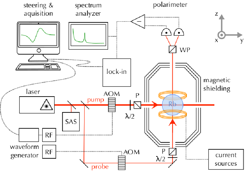
II Experimental Setup
The experimental scheme is shown in Fig. 1. A sample of isotopically-pure 85Rb is contained in a spherical vapor cell of 10 cm diameter, with no buffer gas. The cell is at room temperature (C) corresponding to 85Rb atomic density of atoms/cm3 [16]. The inner cell walls are coated with an antirelaxation (paraffin) layer that prevents atoms from depolarizing upon collision with the walls and prolongs the ground-state Zeeman coherence lifetime to ms.
The cell is inside a “box solenoid,” a cubical box made of printed-circuit-board material, with three mutually perpendicular sets of printed wires, each in a solenoidal pattern. Together with an accompanying ferrite box, which extends the effective length of the solenoid based on the method of images for magneto-statics, we can generate a uniform field along the three directions. In this experiment we generate a constant magnetic field along the -axis, which is also the probe beam direction, while the coils in the perpendicular directions are used to compensate the residual transverse magnetic field. Residual magnetic field gradients are compensated by a set of three mutually perpendicular anti-Helmoltz coils wound around the box. This setup was kept inside three nested layers of -metal shields, giving a whole magnetic shielding of efficiency.
The light source for both probing and pumping is an extended-cavity diode laser whose frequency is stabilized by saturated absorption spectroscopy at MHz below the transition of the 85Rb D1 line (see Section IV). The laser beam is split into pump and probe beams that pass through acousto-optic modulators independently driven by two MHz RF signals so that, before reaching the atoms, the frequency is additionally red-detuned MHz away from the transition. Additionally, the intensity of the pump beam is sinusoidally modulated with frequency . 11 1 The AOM along the probe beam path makes the setup suitable also for single-beam NMOR but is not necessary in the strategy followed in this paper, where just the pump beam needs to be amplitude modulated. Both pump and probe have a beam diameter of mm at the center of the vapor cell.
Both beams are vertically polarized (x-direction in Fig. 1) with high-quality crystal polarizers to ensure pure linear polarization and the light intensity that interacts with the atoms can be adjusted with half-wave plates situated in front of the polarizers. The pump beam passes through the cell in the direction, perpendicular to the -axis bias field. When the pumping modulation frequency coincides with twice the Larmor precession frequency, a large precessing alignment accumulates in the plane (see Section III). The pump power is set to W. The probe beam propagates through the atomic vapor cell along the -axis, i.e. parallel to the field, and experiences Faraday rotation (NMOR) of the polarization plane due to the precessing alignment. The optimal probe power changes from W to W, depending on the employed detector’s gain (see section V).
Polarization rotation is detected with a balanced polarimeter consisting of a Wollaston prism set at an angle of with respect to the vertical and a fiber-coupled variable gain balanced photo-detector (PDB) (Thorlabs PDB150A DC). The differential output is analyzed with a radio-frequency (RF) spectrum analyzer (SA) (RIGOL DSA1030A) or demodulated at with a lock-in amplifier (Stanford Research Systems model SR844). The in-phase and quadrature output signals are then stored on a computer for later analysis. As explained in section IV, both SA and lock-in signals are used to determine the magnetometer sensitivity. Throughout this work we used SA resolution bandwidth RBW Hz and video bandwidth VBW Hz.
III Faraday rotation signal
The AMOR signal is generated by means of amplitude modulated pumping and unmodulated CW probing in a right-angle geometry. Optical pumping with linearly polarized light generates spin alignment, i.e. ground state coherences between Zeeman sub-levels with [42, 43]. The alignment describes a preferred axis, but not a preferred direction along this axis. The signal due to alignment oscillates at twice the Larmor frequency due to this additional symmetry, i.e., at where is the Landé factor and is the Bohr magneton. Amplitude modulated optical pumping at produces a resonant build-up of spin alignment, as demonstrated in several earlier works [17, 28]. The alignment behaves as a damped driven oscillator, and in steady state responds at frequency with an amplitude and phase relative to the drive that depend on the detuning [44]. The weak probe is sensitive to alignment through linear dichroism, i.e., linearly polarized light parallel to the alignment experiences less absorption [3]. When the alignment is neither parallel to nor perpendicular to the probe polarization, this dichroism rotates the probe polarization. This rotation signal also oscillates at , and we demodulate it with the lock-in amplifier to extract the in-phase and quadrature components, shown in Fig. 2 for a representative magnetic field intensity of T.

The optical rotation angle is an oscillating function at the modulation frequency with the amplitude dependence well described by a single-Lorentzian in the small field approximation
| (1) | |||||
where is the maximum rotation angle, which depends on the optical detuning, cell dimension, and pump power. The detuning between the modulation frequency and is while is the FWHM line width due to relaxation, pumping, and nonlinear Zeeman shifts 22 2 The single-Lorentzian approximation should fail at large , when the resonance splits into several lines due to the nonlinear Zeeman shift. This was not observed at the field strengths used in this work. Even at T, the response was well approximated as a single Lorentzian. This suggests a strong line-broadening accompanied the nonlinear Zeeman shift.. The symbols and are the in-phase and quadrature components, respectively, directly observable by demodulation at . The photon shot noise contribution, , is a white noise with a power spectral density [20, 18, 3], where is the flux of photons arriving to the detector.
We note that on resonance, i.e. with , the signal consists of a cosine wave at frequency with amplitude , plus a white-noise background due to . In the balanced condition, and with , the polarimeter signal is . When recorded on a spectrum analyzer with resolution bandwidth , the signal shows a peak power spectral density , where is the gain relating rotation angle to RF amplitude at the SA (the factor of one half represents a mean value of ). A typical RF spectrum of the AMOR resonance recorded in our measurements is shown in Figure 3. The signal peak rises above a flat background , where is the spectral noise density of the phase, so that has units rad/ (the factor of two reflects the fact that only one quadrature contributes to the noise of the demodulated signal, while both are recorded by the SA). The signal-to-noise ratio is given by , which is independent of and and can be directly measured.

The magnetic sensitivity can be related to by noting that the slope of the quadrature component on resonance is
| (2) |
where the width has unit of Hz. Considering that on resonance , we find the noise in magnetic units, i.e., the sensitivity
| (3) |
with units T/.
As described in the next section, using this method to measure the sensitivity we find as low as fT/. For comparison, the atomic projection noise contribution to the overall measurement is: [1, 2]:
| (4) |
where is the number of atoms involved in the measurement. With our cell volume of , cm, atomic density atoms/cm3, measured relaxation rate Hz and s time of measurement we find fT/. This value is two orders of magnitude lower than the observed sensitivity, justifying our earlier step of ignoring this contribution. If all other noise sources have lower amplitude than the shot noise, then the magnetometer can be expected to be photon shot-noise-limited. In Section V we demonstrate that, in the experimental conditions that optimize the sensitivity, this is indeed the case.
IV Optimization of the Magnetometer sensitivity
In this section we examine different setup parameters in order to find the optimal conditions maximising the magnetometric sensitivity.
In our configuration, with a pump and probe of the same frequency, laser tuning affects the pumping efficiency, the rotation signal corresponding to a given degree of atomic alignment, and the probe absorption. In addition, the pump power increases both the amplitude and the width of the rotation signal. To optimize these parameters, we first adjust the gradient fields to minimize the broadening due to magnetic field inhomogeneities [46], and then optimize the laser frequency and pump power to maximize the slope of the AMOR signal. The optimum conditions, which we use throughout this work, occur at the detuning of MHz to the red of the transition and W of pump power.


.
To measure the magnetometric sensitivity for a given probe power and field strength, we first set the detuning and pump power to the optimal values discussed above. We then set a constant current in the solenoidal coil along the -axis, and minimize the width of the AMOR resonance with the help of the gradient coils. Demodulation of the signal yields the in-phase and quadrature components of the resonance versus , as depicted in Fig. 2. By fitting a Lorentzian to these curves, the central resonance modulation frequency () and width are obtained. Keeping then fixed and maximizing the in-phase component allows one to measure the spectrum as in Fig. 3 and to extract . A second spectrum is taken with the B-field set near zero. This moves the resonance peak far away from , so that now gives the background noise . In analogy with previous works [18, 47] the experimental sensitivity, defined by equation 3, can be calculated in terms of the width (FWHM) and signal-to-noise ratio. The magnetometric sensitivity of the instrument was measured in the range from T to T. We employ two detector bandwidths, kHz and MHz, corresponding respectively to nominal transimpedance gains of V/A and V/A.
Typical results, taken at a field of 7.6 T (modulation frequency of kHz, detector gain setting V/A) are shown in Figs. 5 and 5. In Fig. 5 we present signal and noise power spectral densities with the resulting signal-to-noise ratio (SNR) as a function of the probe power. Signal grows with the probe power until saturation occurs. In contrast, noise grows monotonically, so that the SNR has an optimal value before the signal saturates. Fig. 5 depicts the slope and the sensitivity , calculated using equation 3, as a function of probe power, also acquired with T. An optimum sensitivity of 70 fT is observed at a probe power of 80.5 W 33 3 Although this probe power exceeded the pump power of 60 W, the increased resonance broadening is compensated by higher signal amplitude and results in a better net sensitivity. Moreover, for the gain setting of V/A we find the optimal probe power to be as high as 620W. and remains within 10% of this value between 50 W and 100 W 44 4 While optimized sensitivity value of 70 fT is observed below 10.8 T at higher fields this number rises significantly, roughly as , reaching 250 pT at 75 T ( kHz). The observed reduction of the sensitivity for larger fields is related to the nonlinear Zeeman effect (NLZ) [3, 19, 28]. Saturation of the ferrite shielding cube at high fields and high-order magnetic field gradients that are not compensated in the current experimental setup could also contribute to the sensitivity worsening and need further investigation..
V Shot-noise-limited performance
Here we report the results of two noise analyses: the first characterises the probing and detection system, without an atomic contribution. This was performed by probing at the optimal laser detuning but with the pump beam off. The second analysis characterizes the magnetometer under the experimental conditions that optimize the sensitivity, as described in section IV.


In a linear detection system, the noise power of the electronic output will depend on the average light power as
| (5) |
where and are constants. The three terms of this polynomial are the “electronic noise” (stemming, e.g. from the detector electronics), the shot noise, and the “technical noise” contributions, respectively [50, 51]. The laser source can contribute to technical noise, e.g. through power fluctuations if the detection is imbalanced or if its optical elements are unstable. By determining the noise scaling as the function of light intensity, we can identify the dominating noise source. When and , we say the system is shot-noise limited, in the sense that the shot noise is the largest noise contribution. These two inequalities define the range of powers in which the system is SNL. If , the system is not SNL for any power. This definition of SNL can be extended to include more stringent conditions that might arise in applications. For any given , we can consider powers satisfying the inequalities , i.e. powers such that the shot-noise contribution is a factor larger than both the electronic noise and the technical noise contributions. For instance, for , the photonic noise is dB higher than the other two contributions of Eq. (5).
For a given field , and thus the Larmor precession or modulation frequency, the noise of interest is , the noise spectral density at the demodulation frequency . Using the SA we collect output noise spectra for several probe intensities. The data shown in Figs. 7 and 7 reveal the resulting scaling of the noise level. The electronic noise floor in the two Figures differs because of the different employed detector’s gain. In the next step we examine the scaling of the noise level.
For any given detection frequency (that will be the modulation/demodulation frequency in the magnetometer operation mode), we can then fit the polynomial of Eq. (5), and find the range of powers and frequencies over which the detection system is SNL.

In Figure 8 we show an example of this analysis for a detection frequency of kHz. We can see that scaling of the noise amplitude is different for different intensity ranges. The red area represents the SNL range. This is the only power range in which quantum noise reduction via probe squeezing could significantly enhance the magnetometer sensitivity. We find good agreement between the observed shot noise level and the predicted value [50] (in W/Hz): , where is the electron charge, Ohm is the SA input impedance and is detector gain at frequency . Due to impedance matching at the detector, the PDB150A transimpedance gain is only half the nominal value when used with the SA. The frequency dependence can be neglected because our signal frequency of kHz is far below the detector’s 300 kHz nominal 3 dB bandwidth. We thus take V/A, which represents the manufacturer’s specification. The photocurrent is where is the averaged optical power and is the detector quantum efficiency.


After performing the same analysis over all detection frequencies, we report in Figs. 10 and 10 lower () and upper () power limits of the SNL range (red area) versus frequency for two detector settings ( V/A with 300 kHz BW and V/A with 5 MHz BW). According to our previous definition we also show the signficant SNL regions with (light blue area) and (cyan area) that correspond to power regions where the photonic shot-noise is respectively dB and dB above the other noise contributions. Below kHz the detection system is limited by electronic noise i.e. not significantly SNL within the investigated range of light power. It is properly reproduced in Fig. 10, although the data coming from the fit procedure suffer from considerable scattering. The dip in the red curves () at kHz is due to technical noise excess at this frequency (see Fig. 7).
Being interested in the SNL range, we have constrained our AMOR measurements, reported in section IV, to modulation/detection frequencies higher than kHz and thus to magnetic field intensities above T. Above modulation frequency of kHz higher detector BW of 5 MHz needs to be used. Because of the lower gain ( V/A), starting from frequency of kHz the system becomes SNL above W as shown in Fig. 10.
Having determined the SNL range of the detector, we now proceed to characterize the magnetometer noise over this range. We set conditions for an optimized B-field measurement, as described in section IV, and switch off the -field but leave on all other components, including the modulated pumping (in contrast to the measurements described above). We then acquire the noise power spectrum as a function of probe power. We report two representative results that correspond to detector setting with high gain and low gain respectively. Although in our experiment we did not observe any significant difference between the detector and the magnetometric noises, these two features may differ in other experimental conditions where environmental or technical noise sources dominate over the fundamental shot-noise contribution, as reported in previous works [18, 21].

In Fig. 11 we show the magnetometer noise power at kHz ( T) and kHz ( T) as a function of probe power. Fitting both data with of Eq. (5) and knowing the electronic noise coefficient , we find the coefficients and and we can define the shot-noise-limited power range. The difference in power range and reference level between the two representative frequencies is due to the different employed BPD gain. The trend of the noise power is linear, i.e. shot-noise-limited, in the power range of W- W and W mW for kHz and kHz respectively. Within this range the observed noise levels agree with theoretical shot-noise levels, calculated in the same way as for Fig. 8, by taking into account the 10% uncertainty on the detector nominal gain.
Most importantly, the probe power intervals in which the magnetometer sensitivity is not worse than of the maximum (reached at W and W respectively) are well inside a significant photon SNL region with , in which the photonic shot-noise is more than dB above the electronic and technical noise levels. Within this optimal power range, significant sensitivity enhancement can be achieved by using optical polarization squeezing of the probe beam [52]. Indeed, the results of Fig. 11 show that the fundamental light shot-noise contribution dominates the magnetometer noise budget i.e. technical noise and atomic projection noise (Eq. 4) are negligible when the magnetometer sensitivity is optimized at room temperature. Similar SNL performance was observed between T and T, over all the investigated magnetic dynamic range.
VI Conclusions
We have demonstrated a sensitive pump-probe optical magnetometer that is shot-noise limited over the field range T to T. We optimized the system for pump/probe detuning, pump and probe beam powers, and found sensitivity of 70 fT/ at a field of T. The shot-noise-limited performance of the system has been confirmed by the scaling of the magnetometer noise as a function of probe input power and by agreement with the theoretical shot-noise level. This is the first experimental demonstration of a photon shot-noise-limited AMOR magnetometer. Moreover, it has the highest reported sensitivity for a room-temperature optical magnetometer in a range around T. Based on these observations, the described magnetometer is a good candidate for squeezed-light enhancement of sub-pT sensitivity over a broad dynamic range.
It is worth noting that AMOR and other modulated magnetometry strategies at these field strengths are well-matched to atom-resonant sources of squeezed light, because the signal is recovered at a multiple of the Larmor frequency, i.e. at a radio frequency. Although optical squeezing can be generated at low frequencies [53], in practice most squeezing experiments, and to date all atom-resonant squeezed light sources [54, 55, 56, 57, 58], have shown squeezing at radio frequencies.
A number of improvements suggest themselves. The lower limit of T is set by the low-frequency electronic noise of the balanced detector. Electronics designed for lower frequency ranges [53] could make the system shot-noise-limited also for weaker fields. Recently-developed anti-relaxation coatings [59] could extend the ground-state coherence. Techniques to evade broadening due to the nonlinear Zeeman effect could improve the sensitivity at high fields [60, 61, 62].
Acknowledgements
We thank Adam Wojciechowski, R. Jiménez Martínez, F. M. Ciurana and Y.A. de Icaza Astiz for helpful discussions. This work was supported by the Spanish MINECO project MAGO (Ref. FIS2011-23520), European Research Council project AQUMET, Polish National Science Center (2012/07/B/ST2/00251), and by the Foundation for Polish Science (TEAM).
References
- [1] D. Budker, W. Gawlik, D. F. Kimball, S. M. Rochester, V. V. Yashchuk, and A. Weis, Rev. Mod. Phys. 74, 1153 (2002a).
- [2] D. Budker and M. Romalis, Nat Phys 3, 227 (2007).
- [3] D. Budker and D. F. Kimball, eds., Optical Magnetometry (Cambridge University Press, 2013).
- [4] G. Bison, N. Castagna, A. Hofer, P. Knowles, J.-L. Schenker, M. Kasprzak, H. Saudan, and A. Weis, Applied Physics Letters 95, 173701 (2009).
- [5] S. Knappe, T. H. Sander, O. Kosch, F. Wiekhorst, J. Kitching, and L. Trahms, Applied Physics Letters 97, 133703 (2010).
- [6] C. Johnson, P. D. D. Schwindt, and M. Weisend, Applied Physics Letters 97, 243703 (2010).
- [7] B. Ledley, Rev. Phys. Appl. 5, 164 (1970).
- [8] A. W. e. a. E. Luvsandamdin, G. Mura, CLEO EUROPE/EQEC (2011).
- [9] D. Budker, S. K. Lamoreaux, A. O. Sushkov, and O. P. Sushkov, Phys. Rev. A 73, 022107 (2006).
- [10] M. Smiciklas, J. M. Brown, L. W. Cheuk, S. J. Smullin, and M. V. Romalis, Phys. Rev. Lett. 107, 171604 (2011).
- [11] M. Pospelov, S. Pustelny, M. P. Ledbetter, D. F. J. Kimball, W. Gawlik, and D. Budker, Phys. Rev. Lett. 110, 021803 (2013).
- [12] V. Shah, G. Vasilakis, and M. V. Romalis, Phys. Rev. Lett. 104, 013601 (2010).
- [13] F. Wolfgramm, A. Cerè, F. A. Beduini, A. Predojević, M. Koschorreck, and M. W. Mitchell, Phys. Rev. Lett. 105, 053601 (2010a).
- [14] T. Horrom, R. Singh, J. P. Dowling, and E. E. Mikhailov, Phys. Rev. A 86, 023803 (2012).
- [15] LIGO Scientific Collaboration, Nat. Photonics 7, 613 (2013).
- [16] available online at http://steck.us/alkalidata ((revision 2.1.5, 19 September 2012)).
- [17] J. M. Higbie, E. Corsini, and D. Budker, Review of Scientific Instruments 77, 113106 (2006).
- [18] S. Pustelny, A. Wojciechowski, M. Gring, M. Kotyrba, J. Zachorowski, and W. Gawlik, Journal of Applied Physics 103, 063108 (2008).
- [19] V. Acosta, M. P. Ledbetter, S. M. Rochester, D. Budker, D. F. Jackson Kimball, D. C. Hovde, W. Gawlik, S. Pustelny, J. Zachorowski, and V. V. Yashchuk, Phys. Rev. A 73, 053404 (2006).
- [20] D. F. J. Kimball, L. R. Jacome, S. Guttikonda, E. J. Bahr, and L. F. Chan, Journal of Applied Physics 106, 063113 (2009).
- [21] E. Breschi, Z. D. Grujić, P. Knowles, and A. Weis, Applied Physics Letters 104, 023501 (2014).
- [22] S. J. Smullin, I. M. Savukov, G. Vasilakis, R. K. Ghosh, and M. V. Romalis, Phys. Rev. A 80, 033420 (2009).
- [23] I. K. Kominis, T. W. Kornack, J. C. Allred, and M. V. Romalis, Nature 422, 596 (2003).
- [24] D. Sheng, S. Li, N. Dural, and M. V. Romalis, Phys. Rev. Lett. 110, 160802 (2013).
- [25] W. Gawlik, J. Kowalski, R. Neumann, and F. Träger, Optics Communications 12 (issue 4), 400 (1974).
- [26] W. Gawlik, L. Krzemień, S. Pustelny, D. Sangla, J. Zachorowski, M. Graf, A. O. Sushkov, and D. Budker, Applied Physics Letters 88, 131108 (2006).
- [27] D. Budker, D. F. Kimball, V. V. Yashchuk, and M. Zolotorev, Phys. Rev. A 65, 055403 (2002b).
- [28] B. Patton, O. O. Versolato, D. C. Hovde, E. Corsini, J. M. Higbie, and D. Budker, Applied Physics Letters 101, 083502 (2012).
- [29] S. Brandt, A. Nagel, R. Wynands, and D. Meschede, Phys. Rev. A 56, R1063 (1997).
- [30] A. B. M. Irina Novikova and G. R. Welch, J. Opt. Soc. Am. B 22, 44 (2005).
- [31] D. Budker, V. Yashchuk, and M. Zolotorev, Phys. Rev. Lett. 81, 5788 (1998).
- [32] E. P. Corsini, T. Karaulanov, M. Balabas, and D. Budker, Phys. Rev. A 87, 022901 (2013a).
- [33] M. Koschorreck, M. Napolitano, B. Dubost, and M. W. Mitchell, Phys. Rev. Lett. 104, 093602 (2010a).
- [34] M. Koschorreck, M. Napolitano, B. Dubost, and M. W. Mitchell, Phys. Rev. Lett. 105, 093602 (2010b).
- [35] R. J. Sewell, M. Napolitano, N. Behbood, G. Colangelo, and M. W. Mitchell, Nat Photon 7, 517 (2013).
- [36] W. Wasilewski, K. Jensen, H. Krauter, J. J. Renema, M. V. Balabas, and E. S. Polzik, Phys. Rev. Lett. 104, 133601 (2010).
- [37] R. J. Sewell, M. Koschorreck, M. Napolitano, B. Dubost, N. Behbood, and M. W. Mitchell, Phys. Rev. Lett. 109, 253605 (2012).
- [38] G. Vasilakis, V. Shah, and M. V. Romalis, Phys. Rev. Lett. 106, 143601 (2011).
- [39] V. Schultze, R. IJsselsteijn, and H.-G. Meyer, Applied Physics B 100, 717 (2010).
- [40] V. Schultze, R. IJsselsteijn, T. Scholtes, S. Woetzel, and H.-G. Meyer, Opt. Express 20, 14201 (2012).
- [41] The AOM along the probe beam path makes the setup suitable also for single-beam NMOR but is not necessary in the strategy followed in this paper, where just the pump beam needs to be amplitude modulated.
- [42] C. Cohen-Tannoudji, Atomic Physics 4, Plenum Press , p. 589 (1974).
- [43] C. Cohen-Tannoudji, North-Holland Les Houches Summer School (1975).
- [44] J. Z. P. Wlodarczyk, S. Pustelny and M. Lipinski, J. Inst. (IOP Journal of Instrumentation) JINST 7, P07015 (2012).
- [45] The single-Lorentzian approximation should fail at large , when the resonance splits into several lines due to the nonlinear Zeeman shift. This was not observed at the field strengths used in this work. Even at T, the response was well approximated as a single Lorentzian. This suggests a strong line-broadening accompanied the nonlinear Zeeman shift.
- [46] S. Pustelny, D. F. Jackson Kimball, S. M. Rochester, V. V. Yashchuk, and D. Budker, Phys. Rev. A 74, 063406 (2006).
- [47] G. B. S. Groeger and A. Weis, J. Res. Natl. Inst. Stand. Technol. 110, 179 (2005).
- [48] Although this probe power exceeded the pump power of 60 W, the increased resonance broadening is compensated by higher signal amplitude and results in a better net sensitivity. Moreover, for the gain setting of V/A we find the optimal probe power to be as high as 620W.
- [49] While optimized sensitivity value of 70 fT is observed below 10.8 T at higher fields this number rises significantly, roughly as , reaching 250 pT at 75 T ( kHz). The observed reduction of the sensitivity for larger fields is related to the nonlinear Zeeman effect (NLZ) [3, 19, 28]. Saturation of the ferrite shielding cube at high fields and high-order magnetic field gradients that are not compensated in the current experimental setup could also contribute to the sensitivity worsening and need further investigation.
- [50] H.-A. Bachor and T. C. Ralph, A Guide to Experiments in Quantum Optics, edited by Wiley-VCH (2004).
- [51] Y. A. de Icaza Astiz, V. G. Lucivero, R. d. J. León-Montiel, and M. W. Mitchell, Phys. Rev. A 90, 033814 (2014).
- [52] F. Wolfgramm, A. Cerè, F. A. Beduini, A. Predojević, M. Koschorreck, and M. W. Mitchell, Phys. Rev. Lett. 105, 053601 (2010b).
- [53] H. Vahlbruch, S. Chelkowski, B. Hage, A. Franzen, K. Danzmann, and R. Schnabel, Phys. Rev. Lett. 97, 011101 (2006).
- [54] T. Tanimura, D. Akamatsu, Y. Yokoi, A. Furusawa, and M. Kozuma, Opt. Lett. 31, 2344 (2006).
- [55] G. Hétet, O. Glöckl, K. A. Pilypas, C. C. Harb, B. C. Buchler, H.-A. Bachor, and P. K. Lam, Journal of Physics B: Atomic, Molecular and Optical Physics 40, 221 (2007).
- [56] A. Predojevic, Z. Zhai, J. M. Caballero, and M. W. Mitchell, Phys. Rev. A 78, 063820 (2008).
- [57] J. Appel, E. Figueroa, D. Korystov, M. Lobino, and A. I. Lvovsky, Phys. Rev. Lett. 100, 093602 (2008).
- [58] S. Burks, J. Ortalo, A. Chiummo, X. Jia, F. Villa, A. Bramati, J. Laurat, and E. Giacobino, Opt. Express 17, 3777 (2009).
- [59] E. P. Corsini, T. Karaulanov, M. Balabas, and D. Budker, Phys. Rev. A 87, 022901 (2013b).
- [60] V. M. Acosta, M. Auzinsh, W. Gawlik, P. Grisins, J. M. Higbie, D. F. Jackson Kimball, L. Krzemien, M. P. Ledbetter, S. Pustelny, S. M. Rochester, V. V. Yashchuk, and D. Budker, Optics Express, Opt. Express 16, 11423 (2008).
- [61] K. Jensen, V. M. Acosta, J. M. Higbie, M. P. Ledbetter, S. M. Rochester, and D. Budker, Phys. Rev. A 79, 023406 (2009).
- [62] W. Chalupczak, A. Wojciechowski, S. Pustelny, and W. Gawlik, Phys. Rev. A 82, 023417 (2010).