Discrete time ruin probability
with Parisian delayThanks: This work is partially supported by National Science Centre Grant No. DEC-2011/01/B/HS4/00982
(2012-2013). All authors kindly acknowledges partial support by the project RARE -318984, a Marie Curie IRSES Fellowship within the 7th European
Community Framework Programme.
Abstract.
In this paper we evaluate the probability of the discrete time Parisian ruin that occurs when surplus process stays below or at zero at least for some fixed duration of time . We identify expressions for the ruin probabilities within finite and infinite-time horizon. We also find their light and heavy-tailed asymptotics when initial reserves approach infinity. Finally, we calculate these probabilities for a few explicit examples.
Keywords. Discrete time risk process ruin probability asymptotic Parisian ruin.
2000 Mathematics Subject Classification
60J99, 93E20, 60G511. Introduction
In the present paper we consider the following process:
| (1) |
where denotes the initial reserve and
We assume that () are i.i.d. claims and we also assume that premium rate equals to . We denote for and we assume that , hence a.s. The risk process starts from and later we use convention and . The discrete-time model (1) is very important for actuarial practice, since many crucial quantities related to this model have a recursive nature and are readily programmable in practice; see e.g., [39, 49] and references therein.
One of the most important characteristics in risk theory is finite-time ruin probability defined by for the ruin moment and fixed time horizon . Let us note here that our definition is compatible with many papers, see e.g., Gerber [25] and Dickson [17]. Other authors define the ruin moment when the reserve takes strictly negative value (see e.g., Willmot [49]). In this paper we extend this notion to so-called Parisian ruin probability, which occurs if the process stays below or at zero at least for a fixed time period . Formally, we define Parisian ruin time by:
and we consider Parisian ruin probabilities and .
The case corresponds to the classical ruin problem. There are already a number of relevant results analyzing this case, e.g., Dickson and Hipp [22], Gerber and Shiu [26, 27], Li and Garrido [35, 36], Lin and Willmot [37, 38], Shiu [46], Willmot [50]. Moreover, Li et al. in [39] presented a comprehensive review. The discrete model was first proposed by seminal paper of Gerber [25]. In this paper the ruin probability was expressed in terms of total amount of claims cumulated up to time . Explicit formulas for the ruin probability were also derived by Willmot [49] (see also Cheng et al. [8]), where the author used analytical techniques, such as Lagrange’s expansions of moment generating functions.
Other related results concern the expected discounted penalty function (so-called Gerber-Shiu function), corresponding to the joint distribution of the surplus immediately before and at ruin moment. For example Cheng et al. in [8] considered the discounted probability of ruin: , where the surplus just before ruin is , the deficit at ruin equals and is a discount factor . Li and Garrido [34] explored this topic further giving a recursive formula for the expected discounted penalty function due to ruin. In their proof they used the moment generating functions. In continuous-time model a similar approach was applied by Dickson [19]. A detailed discussion was given when the claim size is geometrically distributed. Another approach is based on a defective renewal equation; see Landriault [30], Pavlova and Willmot [43]. Results for the discrete-time risk models were also used as approximations or bounds for the corresponding results in continuous time, see Cossette et al. [11] and Dickson et al. [20] for the approximating procedures. Other references on the related topics are: Cossette et al. [10, 12], Dickson [17, 18], Li [32, 33], Michel [42], Wu and Li [52], Yang et al. [53], Yuen and Guo [54, 55].
The name for the problem considered in this paper is borrowed from Parisian option, where prices are activated or canceled depending on a type of option when underlying asset stays above or below barrier long enough (see Albrecher et al. [1], Chesney et al. [9], Dassios and Wu [14]). We believe that Parisian ruin probability could be a better measure of risk in many situations giving possibility for insurance company to get solvency. So far the Parisian ruin probability has been considered only in a continuous-time setting. In particular, Dassios and Wu [14] analyze the continuous-time classical risk process (1) with exponential claims and the Brownian motion with drift. Dassios and Wu [15] found also Cramér-type asymptotics for this risk process. Czarna and Palmowski [13] and Loeffen et al. [41] extended these results to the case of a general spectrally negative Lévy process using the fluctuation theory. Another possible way of defining the Parisian delay is based on exchanging the deterministic, fixed delay by an independent exponential random variable; see e.g., Landriault et al. [29] and Baurdoux et al. [5].
The main goal of this paper is to derive discrete-time counterparts of the results above and propose efficient numerical procedure for finding Parisian probability of (non-)ruin within finite time.
This paper is organized as follows. In Sections 2 and 3 we give main representation of Parisian non-ruin and ruin probabilities within finite and infinite time respectively. In Sections 4 and 5 we give asymptotics of Parisian ruin probability in Cramér (light-tailed) and heavy-tailed cases. Finally, in Section 6 we analyze a few particular examples.
2. Parisian non-ruin probability over any finite-time horizon
In the main result we will use the following Seal-type formula proved in Lefévre and Loisel [31, Prop. 2.4].
Lemma 1.
We have and for :
| (2) |
where denotes the -th convolution of the law of .
Remark 1.
Lemma 2.
For we have:
Proof.
The first equality is a straightforward consequence of Markov property.
The second equality follows from
decomposition of a trajectory of into two parts and from lemma given in Lefévre and Loisel
[31, Lem. 2.3].
Remark 2.
Assume that the claim is of the form , where is a Bernoulli random variable with and is a geometric random variable with parameter , that is
| (5) |
Model (1) with such distribution of claims is a particular case of widely used compound binomial model. In this model at each unit of time a claim might arrive with probability and there is no claim with probability (see Cheng et al. [8], Li and Guo [40], dos Reis [44]). By lack of memory property of geometric distribution, we have:
Similarly,
Moreover, Wu and Li [52, eq. (4.7)] showed that for the compound binomial model:
where solves for p.g.f of generic claim . In our case of (5) we have and hence
Let
The main representation of the finite-time Parisian ruin probability is given in the next theorem.
Theorem 1.
Proof.
The statement for is obvious. For the Parisian ruin occurs after time if and only if one of the following two separate scenarios happen. In the first one, the classical ruin time happens after time . In the second scenario, we can decompose possible trajectory that drops below zero into two parts. The first part runs until the first time it hits . The second one runs after this time. Precisely, the first piece of this trajectory crosses level at ruin time and it has the undershoot of size . Later it returns to level . This excursion from must have length , otherwise we will have Parisian ruin before time . The second part of the above mentioned trajectory starts at and avoids Parisian ruin over . This observation and the strong Markov property imply formula (1). Equality (7) follows from Kendall’s identity for a random walk (see Alili et al. [2], Bertion [6, Cor. VII.3] and Feller [24, eq. (9.3), p. 424]).
3. Ultimate Parisian ruin probability
Gerber [25], Lefévre and Loisel [31, Cor. 2.8], Shiu [46] and Willmot [49] proved the following result.
Lemma 3.
We have:
| (8) |
Theorem 2.
For the representation of ultimate Parisian ruin probability is given by:
where
| (10) |
4. Cramér’s estimate of the ultimate Parisian ruin probability
In this section we derive the exponential asymptotics of the ultimate Parisian ruin probability when a generic claim size has light-tailed distribution.
For all we define moment-generating function
where is a generic claim size and is an expectation with respect to (we skip subscript if ). We will consider also a dual random walk with a generic increment . Note that . Let be the number of times new maxima are reached within steps of . Let be the number of steps required to achieve new maxima and be the -th new maximum of . In other words, let be a ladder height process of .
Assume Cramér conditions that is: there exists satisfying:
| (11) |
and
| (12) |
Above assumptions mean that for a generic claim size , hence its distribution is light-tailed.
In lemmas below we recall the Cramér asymptotics for the ultimate classical ruin probability. Results follow from random walk theory and renewal theory and as such seem to be classical ones. In the ruin theory for discrete risk process such results are presented e.g., in Landriault et al. [12] (see also Willmot and Lin [51] and Rolski et al. [45, p. 255-259]). However, there exist different representation of the constant used in this results. In most cases, these expressions for contain the ruin probability at . Moreover authors often assume that claim size distribution is non-arithmetic, which is not true in our case (since the span of the distribution equals one). For completeness we decided to present a proof based on Asmussen [3, Th. 13.5.2 and 13.5.3, p. 365] (in a lattice version).
Proof.
By Asmussen [3, Th. 13.5.3, p. 365] it suffices to prove that constant (14) equals to:
| (15) |
For process we can define weakly ascending height process . Note that , where denotes the Dirac’s Delta at . From the Wiener-Hopf factorization (see Asmussen [3, p. 234]):
| (16) |
Moreover, from (16) when we have
| (17) |
To complete the proof we take derivative at of the equation (16). Then we plug its result and (17) into the right-hand side of the equation (15).
Lemma 5.
Proof.
Observe first that:
where . Define Esscher transform via:
| (19) |
for any such that , where is the exponential martingale under . From Asmussen [3, Th.13.5.2 and 13.5.3, p. 365] we have:
Finally, from Asmussen [3, Th. VIII.2.1, p. 224] we obtain:
Let be the inverse of . We are ready now to state the main result of this section.
Theorem 3.
Proof.
To prove Cramér asymptotics (21) we use Lemma 3, equations (2) and (13), where
To prove that function has the Laplace transform (22) observe that:
In the first equality we use summation-by-parts formula. The last equality is a consequence of Optional Stopping Theorem applied to the martingale at the stopping time . Hence, by Lemma 5:
5. Heavy-tailed estimate of the ultimate Parisian ruin probability
In this section we will assume that Cramér equation (11) has no solution. In particular, we assume that the distribution of belongs to the class . We refer to Asmussen and Albrecher [4] and Foss et al. [23] for all properties of these class of distributions; see also Tang et al. [47, 48] and references therein. This class is defined as follows.
Definition 1.
(Class , lattice case of span ) For a parameter we say that distribution function on with tail belongs to class if
-
for each ,
-
Definition 2.
(Class , lattice case of span ) We say that belongs to class if
-
,
-
,
-
for some , we have
(23) where and denotes convolution.
If then we say that is convolution equivalent. The case is particularly interesting since the class is a class of subexponential distributions. If then it is heavy-tailed and its moment generating function does not exist for any strictly positive arguments and therefore right-hand side of (11) is not well-defined. Distributions with regularly varying tails are also in class . Typical example is the Pareto distribution.
Let and , . From now on we will assume that either
| (24) |
or
| (25) |
We recall now the asymptotic result for the ultimate ruin probability.
Proof.
For the case observe that the ruin probability equals the ruin probability for the classical renewal risk process in a continuous time with interarrival time equal and the generic claim size . Then the first part of assertion follows from Asmussen and Albrecher [4, Th. 10.3.1, p. 305] (see also Foss et al. [23, Th. 5.12, p. 113]). The case follows from Bertoin and Doney [7, Th. 1] and Asmussen [3, eq. (4.4.5), p. 231] with
Observe that
and that
where
for a compound Poisson process and being independent of Poisson process with intensity . It is enough to observe this continuous time process at the moments of jumps. We transfer discrete risk process into continuous-time set-up just to use almost straightforward convenient references concerning Lévy processes and to avoid more direct and longer proofs. From Klppelberg and Kyprianou [28, Th. 4.2, eq. (2.8) and Remark 4.3 (iii)] we have that
Lemma 7.
Remark 5.
Note that by Definition 2(ii) for we have and . Unfortunately, it seems that function is very hard to identify more explicitly.
The main result of this section is following.
Theorem 4.
Proof.
Remark 6.
Note that the Parisian delay has influence on the heavy-tailed asymptotics of the ruin probability only when . The subexponential case (when ) gives the same asymptotics as for classical ruin moment , which is a consequence of one big claim that causes the ruin.
6. Examples
In this section we use Theorem 1 to calculate the Parisian non-ruin probability
for various initial capitals and Parisian delays.
We consider classical binomial model (1), where generic claim is a product of Bernoulli random variable with
and
some other positive random variable with values in natural numbers.
To capture different behaviors of the Parisian non-ruin probability, we consider light-tailed case (in Example 1 with geometric d.f. of the claim size)
and heavy-tailed case (in Example 2 with Pareto d.f. of the claim size). In the first case we also found the ultimate non-ruin probability
and compared it with the finite-time one. All numerical calculations have been made in the R package.
Example 1.
In this example we consider generic claim being the product of Bernoulli random variable with and geometric random variable with parameter giving the distribution of the claim size (5). We assume that and . Hence the claim size mean equals which gives positive safety loading.
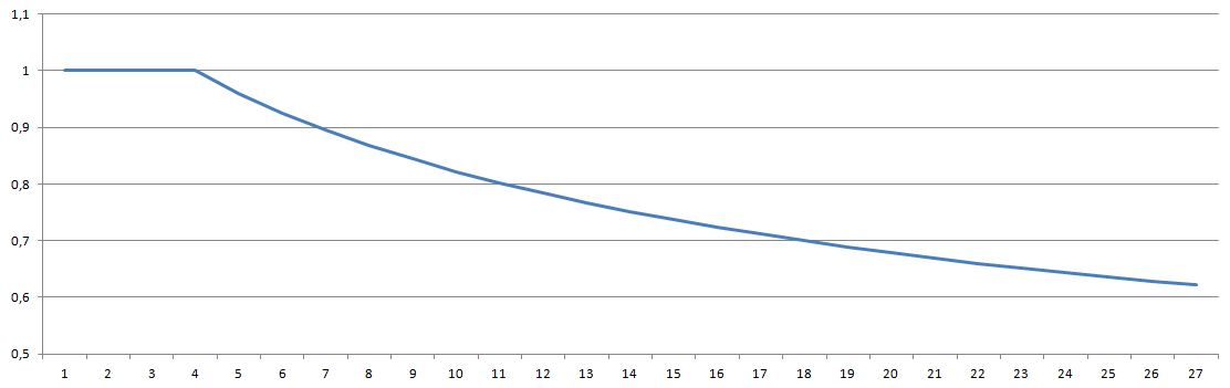
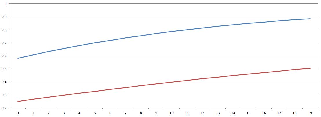
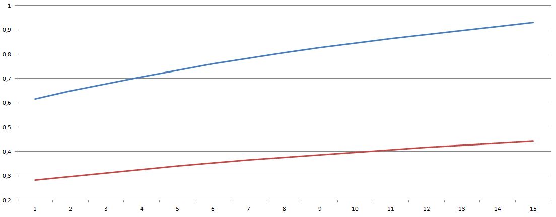
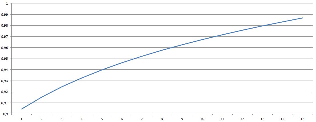
At the beginning we take (initial capital) and (Parisian delay). Table 1 identifies Parisian non-ruin probability for different . All calculations were performed using Theorem 1. Similar result could be derived for the Parisian non-ruin probability for fixed time horizon with different initial capitals (see Table 2 and Figure 2) and for different Parisian delays (see Table 3 and Figure 3). For comparison we also added ultimate non-ruin probability which was found using Remark 2 and Theorem 2. Note that the difference between these two quantities gives the probability of ruin after or at time . In Figures 2 and 3 we use red color to denote ultimate non-ruin probability, and blue color to denote the non-ruin probability over finite-time horizon.
All these calculations show that the formula given in Theorem 1
produces deep comparison results for very wide choice of parameters.
In particular, they demonstrate that increasing the Parisian delay can substantially decrease the ruin probability, while keeping initial capital fixed.
Moreover, considering the difference , it seems plausible that the ruin will happen after time and hence after long time evolution of the risk process (1).
Example 2.
To analyze the heavy-tailed case in this the example, we consider generic claim being the product of Bernoulli random variable with and Pareto random variable . That is, we have:
Note that then , where is Riemann zeta function. To obtain as it was in the previous example, we take .
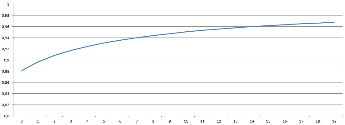
In the tables and figures below, we show how the Parisian non-ruin probability changes for different time horizons (Table 4 and Figure 4 with (initial capital), (Parisian delay)), different initial capitals (Table 5 and Figure 5 with (Parisian delay) and (time horizon)) and different Parisian delays (Table 6 and Figure 6 with (initial capital) and (time horizon)).
In the heavy-tailed case, the non-ruin Parisian probability is much bigger than in the light-tailed case. At the same time in the heavy-tailed case, the loss given default is substantially larger.
| Time t | |
|---|---|
| 1..4 | 1 |
| 5 | 0,959785 |
| 6 | 0,925200 |
| 7 | 0,894939 |
| 8 | 0,868044 |
| 9 | 0,843803 |
| 10 | 0,821846 |
| 11 | 0,801862 |
| 12 | 0,783589 |
| 13 | 0,766809 |
| 14 | 0,751338 |
| 15 | 0,737022 |
| 16 | 0,723729 |
| 17 | 0,711349 |
| 18 | 0,699784 |
| 19 | 0,688951 |
| 20 | 0,678780 |
| 21 | 0,669207 |
| 22 | 0,660177 |
| 23 | 0,651642 |
| 24 | 0,643560 |
| 25 | 0,635894 |
| 26 | 0,628609 |
| 27 | 0,621676 |
Results of table above were also presented on Figure 1.
| u | |||
|---|---|---|---|
| 0 | 0,5810479 | 0,249772 | 0,3312759 |
| 1 | 0,607774 | 0,266081 | 0,3416928 |
| 2 | 0,632917 | 0,282036 | 0,3508806 |
| 3 | 0,656559 | 0,297644 | 0,3589148 |
| 4 | 0,678780 | 0,312913 | 0,3658669 |
| 5 | 0,699656 | 0,327849 | 0,3718072 |
| 6 | 0,719260 | 0,342461 | 0,3767995 |
| 7 | 0,737663 | 0,356756 | 0,3809066 |
| 8 | 0,754929 | 0,370739 | 0,3841904 |
| 9 | 0,771124 | 0,384418 | 0,3867056 |
| 10 | 0,786308 | 0,397801 | 0,3885074 |
| 11 | 0,800539 | 0,410892 | 0,3896471 |
| 12 | 0,813871 | 0,423699 | 0,3901725 |
| 13 | 0,826358 | 0,436227 | 0,3901309 |
| 14 | 0,838048 | 0,448483 | 0,3895649 |
| 15 | 0,848989 | 0,460473 | 0,3885157 |
| 16 | 0,859225 | 0,472202 | 0,3870228 |
| 17 | 0,868799 | 0,494899 | 0,3738986 |
| 18 | 0,877750 | 0,483675 | 0,3940752 |
| 19 | 0,886117 | 0,505880 | 0,3802373 |
| 1 | 0,615985 | 0,283120 | 0,332865 |
|---|---|---|---|
| 2 | 0,648228 | 0,298331 | 0,349897 |
| 3 | 0,678780 | 0,312913 | 0,365867 |
| 4 | 0,707581 | 0,326841 | 0,380740 |
| 5 | 0,734634 | 0,340117 | 0,394517 |
| 6 | 0,759986 | 0,352754 | 0,407232 |
| 7 | 0,783716 | 0,364778 | 0,418938 |
| 8 | 0,805913 | 0,376220 | 0,429693 |
| 9 | 0,826625 | 0,387117 | 0,439508 |
| 10 | 0,845859 | 0,397502 | 0,448357 |
| 11 | 0,863890 | 0,407412 | 0,456479 |
| 12 | 0,881019 | 0,416880 | 0,464139 |
| 13 | 0,897518 | 0,425939 | 0,471579 |
| 14 | 0,913656 | 0,434617 | 0,479039 |
| 15 | 0,929708 | 0,442944 | 0,486764 |
| Time t | |
|---|---|
| 1..4 | 1 |
| 5 | 0,991491 |
| 6 | 0,984043 |
| 7 | 0,977390 |
| 8 | 0,971360 |
| 9 | 0,965837 |
| 10 | 0,960746 |
| 11 | 0,956030 |
| 12 | 0,951638 |
| 13 | 0,947532 |
| 14 | 0,943676 |
| 15 | 0,940047 |
| 16 | 0,936617 |
| 17 | 0,933368 |
| 18 | 0,930281 |
| 19 | 0,927343 |
| 20 | 0,924540 |
| 21 | 0,921860 |
| 22 | 0,919294 |
| 23 | 0,916834 |
| 24 | 0,914470 |
| 25 | 0,912195 |
| 26 | 0,910005 |
| 27 | 0,907892 |

| u | |
|---|---|
| 0 | 0,881454 |
| 1 | 0,896836 |
| 2 | 0,908254 |
| 3 | 0,917233 |
| 4 | 0,924540 |
| 5 | 0,930631 |
| 6 | 0,935802 |
| 7 | 0,940255 |
| 8 | 0,944135 |
| 9 | 0,947548 |
| 10 | 0,950576 |
| 11 | 0,953289 |
| 12 | 0,955714 |
| 13 | 0,957914 |
| 14 | 0,959912 |
| 15 | 0,961735 |
| 16 | 0,963406 |
| 17 | 0,964943 |
| 18 | 0,966360 |
| 19 | 0,967673 |
| 1 | 0,904499 |
|---|---|
| 2 | 0,915302 |
| 3 | 0,92454 |
| 4 | 0,932625 |
| 5 | 0,939821 |
| 6 | 0,946308 |
| 7 | 0,952214 |
| 8 | 0,957633 |
| 9 | 0,962638 |
| 10 | 0,967283 |
| 11 | 0,971624 |
| 12 | 0,975709 |
| 13 | 0,979579 |
| 14 | 0,983266 |
| 15 | 0,986801 |
References
- [1] Albrecher, H., Kortschak, D. and Zhou, X. (2012) Pricing of Parisian options for a jump-diffusion model with two-sided jumps. Appl. Math. Fin. 19(2).
- [2] Alili, L., Chaumont, L. and Doney, R. (2005) On a fluctuation identity for random walks and Lévy processes. Bull. Lond. Math. Soc 37, 141–148.
- [3] Asmussen, S. (2003) Applied Probability and Queuees. Springer.
- [4] Asmussen, S. and Albrecher, H. (2010) Ruin Probabilities. World Scientific, Singapore.
- [5] Baurdoux, E.J. , Pardo, J.C., Pérez, J.L., and Renaud J.-F. (2015) Gerber-Shiu functionals at Parisian ruin for Lévy insurance risk processes. Adv. Appl. Probab. (in press).
- [6] Bertoin, J. (1996) Lévy processes. Cambridge University Press, Cambridge.
- [7] Bertoin, J. and Doney, R. (1996) Some Asymptotic Results for Transient Random Walks. Adv. Appl. Probab. 28(1), 207–226.
- [8] Cheng, S., Gerber, H. U. and Shiu, E.S.W. (2000) Discounted probabilities and ruin theory in the compound binomial model. Insurance Math. Econom. 26, 239–250.
- [9] Chesney, M., Jeanblanc-Picqué, M. and Yor, M. (1997) Brownian excursions and Parisian barrier options. Adv. in Appl. Probab. 29(1), 165-184.
- [10] Cossette, H., Landriault, D. and Marceau, E. (2003) Ruin probabilities in the compound Markov binomial model. Scand. Actuar. J. 4, 301–323.
- [11] Cossette, H., Landriault, D. and Marceau, E. (2004) Compound binomial risk model in a Markovian environment. Insurance Math. Econom. 35, 425–443.
- [12] Cossette, H., Landriault, D. and Marceau, E. (2006) Ruin probabilities in the discrete time renewal risk model. Insurance Math. Econom. 38, 309–323.
- [13] Czarna, I. and Palmowski, Z. (2011) Ruin probability with Parisian delay for a spectrally negative Lévy risk process. J. Appl. Probab. 48(4), 984–1002.
- [14] Dassios, A. and Wu, S. (2009) Parisian ruin with exponential claims. Submitted for publication, see http://stats.lse.ac.uk/angelos/.
- [15] Dassios, A. and Wu, S. (2009) Ruin probabilities of the Parisian type for small claims. Submitted for publication, see http://stats.lse.ac.uk/angelos/.
- [16] De Vylder, F.E. and Goovaerts, M.J. (1988) Recursive calculation of finite-time ruin probabilities. Insurance Math. Econ., 7, 1–7.
- [17] Dickson, D.C.M. (1994) Some comments on the compound binomial model. Astin Bull. 24, 33–45.
- [18] Dickson, D.C.M. (2005) Insurance Risk and Ruin. Cambridge University Press, Cambridge.
- [19] Dickson, D.C.M. (1992) On the distribution of surplus prior to ruin. Insurance Math. Econom. 11, 191–207.
- [20] Dickson, D.C.M., dos Reis, E.A.D. and Waters, H.R. (1995) Some stable algorithms in ruin theory and their applications. Astin Bull. 25, 153–175.
- [21] Dickson, D.C.M. and Waters, H.R. (1991) Recursive calculation of survival probabilities, ASTIN Bulletin, 21, 199–221.
- [22] Dickson, D.C.M. and Hipp, C. (2001) On the time to ruin for Erlang(2) risk process. Insurance Math. Econom. 29, 333–344.
- [23] Foss, S., Korshunov, D. and Zachary, S. (2011) An Introduction to Heavy-Tailed and Subexponential Distributions. Springer.
- [24] Feller W. (1966) An Introiluction to Probubility Theory and its Applications, Vol. II (Wiley, New York)
- [25] Gerber, E. (1988) Mathematical fun with the compound binomial process. ASTIN Bulletin 18, 161–168.
- [26] Gerber, H.U. and Shiu, E.S.W. (1998) On the time value of ruin. N. Am. Actuar. J. 2(1), 48–78.
- [27] Gerber, H.U. and Shiu, E.S.W. (2005) The time value of ruin in a Sparre Andersen model. N. Am. Actuar. J. 9(2), 49–69.
- [28] Klppelberg, C. and Kyprianou, A. (2006) On extreme ruinous behaviour of Lévy insurance risk process. J. Appl. Probab. 43(2), 594–598.
- [29] Landriault, D., Renaud, J.F. and Zhou, X. (2013) Insurance risk models with Parisian implementation delays. Method. Comp. Appl. Probab..
- [30] Landriault, D. (2008) On a generalization of the expected discounted penalty function in a discrete-time insurance risk model. Appl. Stoch. Models Bus. Ind. 24, 525–539.
- [31] Lefévre, C. aned Loisel, S. (2008) On finite-time ruin probabilities for classisal risk models. Scand. Actuarial J. 1, 41–60.
- [32] Li, S. (2005) On a class of discrete-time renewal risk models. Scand. Actuar. J. 4, 241–260.
- [33] Li, S. (2005) Distributions of the surplus before ruin, the deficit at ruin and the claim causing ruin in a class of discrete time risk models. Scand. Actuar. J. 4, 271–284.
- [34] Li, S. and Garrido, J. (2002) On the time value of ruin in the discrete time risk model. Working paper 02-18, Business Economics, University Carlos III of Madrid.
- [35] Li, S. and Garrido, J. (2004) On ruin for Erlang(n) risk process. Insurance Math. Econom., 34, 391–408.
- [36] Li, S. and Garrido, J. (2005) On a general class of renewal risk process: Analysis of the Gerber-Shiu penalty function. Adv. in Appl. Probab. 37, 836–856.
- [37] Lin, X.S. and Willmot, G.E. (1999) Analysis of a defective renewal arising in ruin theory. Insurance Math. Econom. 25, 63–84.
- [38] Lin, X.S. and Willmot, G.E. (2000) The moments of the time of ruin, the surplus before ruin and the deficit at ruin. Insurance Math. Econom. 27, 19–44.
- [39] Li, S., Lu, Y. and Garrido, J. (2009) A review of discrete-time risk models. R ACSAM - Revista de la Real Academia de Ciencias Exactas, Fisicas y Naturales. Serie A. Matematicas 103(2), 321–337.
- [40] Liu, S.X. and Guo, J.Y. (2006) Discrete Risk Model Revisited. Methodology and Computing in Applied Probability, 8(2), 303–313.
- [41] Loeffen, R., Czarna, I. and Palmowski, Z. (2013) Parisian ruin probability for spectrally negative Lévy processes. Bernoulli 19(2), 599–609.
- [42] Michel, R. (1989) Representation of a time-discrete probability of eventual ruin. Insurance Math. Econom. 8, 149–152.
- [43] Pavlova, K. and Willmot, G.E. (2004) The discrete stationary renewal risk model and the Gerber-Shiu discounted penalty function. Insurance Math. Econom. 35, 267–277.
- [44] dos Reis A. E. (1993) The compound binomial model revisited. Manuscript.
- [45] Rolski, T., Schmidli, H., Schmidt, V. and Teugels, J.L. (1999) Stochastic processes for insurance and finance. John Wiley and Sons, Inc., New York.
- [46] Shiu, E. (1989) The probability of eventual ruin in the the compound binomial model. ASTIN Bulletin 19, 179–190.
- [47] Tang, Q. (2006) On convolution equivalence with applications. Bernoulli 12(3), 535–549.
- [48] Tang, Q. and Tsitsiashvili, G. (2003) Precise estimates for the ruin probability in finite horizon in a discrete-time model with heavy-tailed insurance and financial risks. Stochastic Processes and Their Applications 108(2), 299–325.
- [49] Willmot, G.E. (1993) Ruin probabilities in the compound binomial model. Insurance: Mathematics and Economics 12, 133–142.
- [50] Willmot, G.E. (1999) A Laplace transform representation in a class of renewal queueing and risk processes. J. Appl. Probab. 36, 570–584.
- [51] Willmot, G.E. and Lin, X.S. (2001) Lundberg Approximations for Compound Distributions with Insurance Applications. Lecture notes in statistics. Springer-Verlag, New York.
- [52] Wu, X. and Li, S. (2009) On the Gerber-Shiu function in a discrete time renewal risk model with general inter-claim times. Scand. Actuar. J. 4, 281–294.
- [53] Yang, H., Zhang, Z. and Lan, C. (2009) Ruin problems in a discrete Markov risk model. Statistics and Probability Letters 79, 21–28.
- [54] Yuen, K.C. and Guo, J. (2001) Ruin probabilities for time-correlated claims in the compound binomial model. Insurance Math. Econom. 29, 47–57.
- [55] Yuen, K.C. and Guo, J. (2006) Some results on the compound binomial model. Scand. Actuar. J. 3, 129–140.