The Gaia-ESO Survey: the Galactic Thick to Thin Disc transitionThanks: Based on observations collected with the FLAMES spectrograph at the VLT/UT2 telescope (Paranal Observatory, ESO, Chile), for the Gaia-ESO Large Public Survey, programme 188.B-3002
Abstract
Aims. The nature of the Thick Disc and its relation with the Thin Disc is presently an important subject of debate. In fact, the structural and chemo-dynamical transition between disc populations can be used as a test of the proposed models of Galactic disc formation and evolution.
Methods. We have used the atmospheric parameters, abundances and radial velocities, determined from the Gaia-ESO Survey GIRAFFE spectra of FGK-type stars (first nine months of observations), to provide a chemo-kinematical characterisation of the disc stellar populations. We focuss on a subsample of 1016 stars with high quality parameters, covering the volume 4.5 kpc and R in the range 2-13 kpc.
Results. We have identified a thin to thick disc separation in the v.s. plane, thanks to the presence of a low-density region in the number density distribution. The thick disc stars seem to lie in progressively thinner layers above the Galactic plane, as metallicity increases and decreases. On the contrary, the thin disc population presents a constant value of the mean distance to the Galactic plane at all metallicities. In addition, our data confirm the already known correlations between Vϕ and for the two discs. For the thick disc sequence, a study of the possible contamination by thin disc stars suggests a gradient up to 649 km s-1 dex-1. The distributions of azimuthal velocity, vertical velocity, and orbital parameters are also analysed for the chemically separated samples. Concerning the gradients with galactocentric radius, we find, for the thin disc, a flat behaviour of the azimuthal velocity, a metallicity gradient equal to -0.0580.008 dex kpc-1 and a very small positive gradient. For the thick disc, flat gradients in and are derived.
Conclusions. Our chemo-kinematical analysis suggests a picture in which the thick disc seems to have experienced a settling process, during which its rotation increased progressively, and, possibly, the azimuthal velocity dispersion decreased. At -0.25 dex and 0.1 dex, the mean characteristics of the thick disc in vertical distance to the Galactic plane, rotation, rotational dispersion and stellar orbits eccentricity are in agreement with that of the thin disc stars of the same metallicity, suggesting a possible connection between these two populations at a certain epoch of the disc evolution. Finally, the results presented here, based only on the first months of the Gaia ESO Survey observations, confirm how crucial are today large high-resolution spectroscopic surveys outside the solar neighbourhood for our understanding of the Milky Way history.
Key Words.
The Galaxy: abundances, disk, stellar content - Stars: abundances1 Introduction
Understanding the chemodynamical evolution of the Milky Way disc stellar populations is a crucial step to reconstruct the history of our Galaxy. This approach can shed new light on the detailed processes that led the Milky Way to form and evolve as a disc-type galaxy, in the more general context of galaxy evolution. In particular, since the first works highlighting the existence of the Milky Way’s thin/thick disc dichotomy (Yoshii, 1982; Gilmore & Reid, 1983), the study of the structural and chemodynamical transition between the two disc populations has opened new pathways to constraint Galactic evolution models. External mechanisms, supported by the hierarchical formation of galaxies in the CDM paradigm, have been invoked to explain the chemodynamical characteristics of thick disc stars. Among them, the accretion of dwarf galaxies (Statler, 1988; Abadi et al., 2003, e.g.) and minor mergers of satellites (Quinn et al., 1993; Villalobos & Helmi, 2008, e.g.) heating dynamically the disc, have been proposed. Similarly, Jones & Wyse (1983) and Brook et al. (2004); Brook et al. (2007) have proposed the accretion of a gas-rich merger from the collapse of which the thick disc would have formed. On the other hand, purely internal formation mechanisms have also been proposed, like the early turbulent phase of the primordial disc (Bournaud et al., 2009, e.g.) and the stars radial migration due to resonances with the spiral structure or the bar of the Milky Way (Schönrich & Binney, 2009c; Minchev & Famaey, 2010; Loebman et al., 2011, e.g.). The relative importance of the different proposed physical processes of evolution can now be tested with increasing robustness, thanks to the Galactic spectroscopic surveys targeting the disc stars.
Spectroscopic studies of the disc populations were initially based on kinematically selected samples of solar neighbourhood stars (Prochaska et al., 2000; Fuhrmann, 2004; Bensby et al., 2005; Reddy et al., 2006, e.g.), with some exceptions like Edvardsson et al. (1993) or Fuhrmann (1998). In the classical picture that emerged from those studies, the thick disc population is characterized, compared to the thin disc one, as kinematically hotter (Casetti-Dinescu et al., 2011), and therefore, composed by stars moving in Galactic orbits with a higher scale height (Jurić et al., 2008, 900 pc vs. 300 pc, e.g.). In addition, the thick disc metallicity distribution peaks at lower values (Wyse & Gilmore, 1995; Kordopatis et al., 2011; Lee et al., 2011b, -0.5 dex compared to -0.2 dex for the thin disc, e.g). With respect to the thin disc, the thick disc stars are older and have an enhanced ratio of -element abundances over iron (Bensby et al., 2005; Bensby et al., 2007; Fuhrmann, 2008, , e.g.). Nevertheless, it progressively appeared that the distributions in the above mentioned physical parameters displayed significant overlaps between the thin and the thick disc populations (Bensby & Feltzing, 2010, e.g.). This blurred our comprehension of the interplay between the discs and questionned the classical kinematically-based definitions (Bovy et al., 2012c).
On the other hand, as discussed in Bovy et al. (2012b), defining stellar populations by abundances patterns is a better approach than the traditional kinematical criteria, as chemical abundances can correlate with disc structure, but are formally independent of it. Moreover, the identification of possible chemical evolutionary paths and/or gaps in the abundance ratios distributions can be crucial to disentangle the otherwise overlapping populations in the kinematical space.
In the recent years, the number of stars analysed with high enough spectroscopic resolution
to provide detailed chemical diagnostics has increased from a few hundreds to several tens
of thousands.
The advent of Milky Way spectroscopic
surveys and of automatised chemical analysis techniques have improved both the statistical robustness
and the homogeneity of the data as a consequence. From the theoretical side, new approaches based, at least partially,
on the chemical identification of disc sub-populations, as the chemical-tagging (Freeman & Bland-Hawthorn, 2002) or
the mono-abundance populations (Rix & Bovy, 2013) methods, are opening promising pathways for constraining
the Milky Way’s evolutionary processes. This is also challenging our previous conception of the Milky Way disc and
the way in which stellar populations can be defined.
In this context, the low resolution (R 2 000) SEGUE spectroscopic survey addressed the question of the thin to thick disc transition with a robust statistical approach, inside and outside the solar neighbourhood. Lee et al. (2011b) analysed 17 300 G-type dwarfs with errors of about 0.23 dex in [Fe/H] (Smolinski et al., 2011) and 0.1 dex for (Lee et al., 2011a). This was complemented by Schlesinger et al. (2012) who analysed 24 270 G and 16 847 K dwarfs at distances from 0.2 to 2.3 kpc from the Galactic plane. The Lee et al. (2011b) versus [Fe/H] distribution of number densities (see their Fig. 2) already motivated the authors to chemically separate the thin and the thick disc populations, although no clear gap is observed between the two. The SEGUE data interpretations differ from authors proposing no thin-thick disc distinction (Bovy et al., 2012b) to those allowing the existence of a distinct thick-disc component formed through an external mechanism (Liu & van de Ven, 2012). Nevertheless, selection effects have been invoked to explain some of the distinctions between the Lee et al. (2011a) and the Bovy et al. (2012b) chemical distributions. On the other hand, the data interpretation in the sense of no thin-thick disc distinction agrees with the results of the Schönrich & Binney (2009a) theoretical study.
More recently, Boeche et al. (2013) analysed the chemo-kinematical characteristics of 9 131 giants included in the last RAVE survey data release, with available and . The RAVE survey data have a higher resolution (R7 500) than SEGUE spectra, but with a wavelength range limited to the infrared Ca II triplet. The Boeche et al. (2013) analysis, based on the eccentricity-Zmax plane combined with additional orbital parameters, allowed them to identify three stellar populations that could be associated with the Galactic thin disc, a dissipative component composed mostly of thick-disc stars, and the halo. Nevertheless, their thin and thick disc populations, defined with the above mentioned dynamical criteria, do not clearly separate in their v.s. plane (c.f. their Fig. 10).
On the other hand, recent studies of solar neighbourhood samples, analysed with high resolution spectroscopic data, have revealed the existence of a gap in the versus [Fe/H] plane (Fuhrmann, 2004; Reddy et al., 2006; Bensby et al., 2007, e.g). Recently, Adibekyan et al. (2013) used the stellar sample of 1 111 long-lived FGK dwarf stars from Adibekyan et al. (2012) to separate and characterise the different Galactic stellar subsystems, taking into account the existence of the above mentioned gap. Their measurements are based on Mg, Si and Ti averaged abundances and the typical relative uncertainties in the metallicity and are of about 0.03 dex. Haywood et al. (2013) derived ages of the Adibekyan et al. (2012) sample, concluding that two regimes appear in the age- plane, that they identify as the epochs of the thick and thin disc formation. In the Haywood et al. (2013) scenario, the thick disc “formed from a well mixed interstellar medium, probably first in starburst, then in a more quiescent mode, over a time scale of 4-5 Gyr”. They also suggest that “the youngest thick disk set the initial conditions from which the inner thin disk started to form 8 Gyr ago, at [Fe/H] in the range of (-0.1,+0.1) dex and =0.1 dex”. Finally, they interpret the low-metallicity tail of the thin disc as having an outer disc origin, somewhat disconnected from the inner disc evolution. In addition, similar separations in the versus [Fe/H] plane are distinguishable in the Ramírez et al. (2013) oxygen-abundance versus [Fe/H] measurements. These authors also report similar age- regimes as in Haywood et al. (2013).
In summary, the increasing number of Galactic disc stars with known kinematical and chemical characteristics has emphasized the question of the continuity or not between the thick and the thin disc components, in structural properties, kinematics, abundances and ages. Different authors like Norris (1999) and Bovy et al. (2012b) have even raised the possibility of considering the Galactic disc as a single component, without a thick/thin disc distinction, analysing for instance the mass-weighted scale-height distribution of disc stars.
In this context, the GIRAFFE observations of the Gaia-ESO Survey (Gilmore et al., 2012, GES,) offer a unique opportunity to extend the previously high-resolution studies of the solar neighbourhood to larger and more radially extended samples. In its first data release, GES already includes 10 000 spectra (R20 000 and R16 000) of stars in the Milky Way field, from the halo, the thick disc, the thin disc and the bulge. The expected final number of targets, at the end of the five years of observations, is 100 000.
The present paper addresses the thick-thin disc transition as seen in the GES kinematical and chemical ( and global metallicity) first release data of FGK-type stars. Our point of view, exploiting the high resolution of the GES data, is that of the chemical characterisation and definition of the disc populations (essentially identified as thin and thick discs). As a consequence, the subsequent analysis of the structural properties, kinematics and orbital parameters will be done in the framework of the chemically defined disc populations. Section 2 describes the data sample, including the stellar parameters and measurements. Section 3 presents the derivation of the stellar distances and kinematics. Section 4 focuses on the analysis of the number density distribution in the versus plane. Then, the distributions of the distances to the Galactic plane (Section 5), of the azimuthal velocities (Section 6), the azimuthal and vertical velocity dispersions (Section 7) and the stellar orbital parameters (Section 8) are discussed, in the context of a proposed thick-thin disc separation based on the chemical criteria. Section 9 presents the rotational and abundance gradients with galactocentric radius and, finally, we discuss our results in Section 10.
2 The GES data sample, the stellar parameters and the measurements.
The present work is based on the data collected by the Gaia-ESO Survey during the first nine months of observations. As explained in Gilmore et al. (2012), the GES consortium has a work package structure that manages the data flows, from target selection, through data reduction, spectrum analysis, astrophysical parameters determination, calibration and homogenisation, to delivery of science data for verification analysis. The general data processing is described in Gilmore et al. (2014, in preparation).

In this paper, we analyse the iDR1 GES results for 5 000 Milky Way disc field stars observed with the GIRAFFE spectrograph: 4 534 stars observed with both the HR10 (R19 800) and the HR21 (R16 200) setup modes, and 394 stars with only HR10 spectra. Fig. 1 shows the l and b coordinates for the lines of sight of the GES iDR1 (bulge and star clusters fields are excluded). All the targets were selected from Visible and Infrared Survey Telescope for Astronomy (VISTA) photometry. As explained in Gilmore et al. (2012), the target selection for the Halo and disc targets is based on the Disc/Halo transition seen in the Sloan Digital Sky Survey photometry at 17 18 and 0.2 0.4. The equivalent selection from VISTA near-infrared photometry is used by GES with two main selection boxes:
- •
Blue box: 0.0 J-K 0.45 and 14.0 J 17.5 mag
- •
Red box: 0.4 J-K 0.70 and 12.5 J 15.0 mag
The colour boxes are shifted according to the Schlegel extinction maps (Schlegel et al., 1998a). In addition, when the stellar density was not enough to fill in all the FLAMES fibers, as for high latitude fields, the red box was extended to around J-K 0.85 and J17 mag to allow for second priority fibers. The spectrum analysis has shown that the blue box has mainly selected dwarf stars with Teff between 6500 K and 5250 K. The corresponding metallicity distribution peaks at around -0.6 dex for high latitude fields (30) and at -0.3 dex for low latitude fields. On the other hand, the red box has targeted dwarfs with Teff between 6000 K and 4500 K and a small number of giant stars. The metallicity distribution of the red box targets is quite independent on the latitude and it peaks around -0.4 dex. Finally, the extention of the selection boxes in the low density fields has added main sequence dwarfs with Teff between 6000 K and 4000 K with a doubled peaked metallicity distribution (peaks at -0.8 dex and -0.3 dex). The signal to noise value of this second priority targets is in general lower than the main targets data. As a consequence of the selection criteria, the thin disc is preferentially targeted in the low latitude fields with respect to the thick disc, in a proportion of about 3:1, against about 1:1 for the high latitude fields.
The radial velocity measurements are based on a spectral fitting technique, that includes a first guess determination of atmospheric parameters. The method is described in detail by Koposov (2014, in preparation). Typical errors in radial velocity are of the order of 0.3 km/s. The stellar atmospheric parameters and abundances were determined by the GES work package in charge of the GIRAFFE spectrum analysis for FGK-type stars. The final recommended effective temperatures (Teff), surface gravities (), global metallicities () and abundances () were estimated thanks to the combination of three different procedures: MATISSE (Recio-Blanco et al., 2006), FERRE (Allende Prieto et al., 2006, and further developments) and SME (Valenti & Piskunov, 1996, and further developments). The relative error distributions peak at 70 K for Teff, 0.10 dex for , 0.08 dex for and 0.03 dex for . The homogeneity of the parameters between the stars observed with HR10 and HR21 and those observed with HR10 only was verified during the GES parameters validation process. The adopted reference solar abundances are those of Grevesse et al. (2007) and the Gustafsson et al. (2008) MARCS model atmospheres were used for the analysis. For more details about the related GES parametrisation pipeline we refer the reader to Recio-Blanco et al. (2014). In addition, 95% of the targets have proper motions available from the PPMXL catalogue (Roeser et al., 2010) with typical errors of 8 mas/yr.
Fig. 2 shows the Hertzsprung-Russel diagram of the analysed sample of 4 928 GES stars, colour coded by metallicity. Dwarfs stars represent about 74% of the total sample.

2.1 The global estimations
The GES estimations used in this paper were determined, at the same time as the stellar atmospheric parameters, by the three above mentioned groups with different methodologies (Recio-Blanco et al., 2014). More particularly, the final GES iDR1 values are the mean of the three independent determinations: the FERRE and the MATISSE estimations, based on a four dimensional (Teff, , , and ) grid of synthetic spectra (see de Laverny et al., 2012, for a description of the methodologies adopted for this grid); and the SME determination, based on a mean of the preliminary individual abundance estimations of Mg, Ca, Ti and Si. This global is estimated in the first analysis phase, together with Teff, and , and before the final GES recommended individual abundances are determined.
As explained in Recio-Blanco et al. (2014), the final global reflects the information on the -element abundances present in the analysed wavelength ranges for each type of star and spectrum quality. This approach, similar to the SDSS/SEGUE one described by Lee et al. (2011c), estimates the overall -elements behaviour. The relation between the GES iDR1 global and the individual -element abundances, also included in the GES iDR1 (Mg, Ca, Ti and Si), is presented in Recio-Blanco et al. (2014). This analysis shows that the global is dominated by the Mg abundance, with a standard deviation of the difference equal to 0.069 dex.
Finally, GES iDR1 measurements of the Fe abundance are also available, although they are not used in this paper. The relation between and [Fe/H] has also been verified and it is presented in Recio-Blanco et al. (2014). The standard deviation of the difference between and [Fe/H] is 0.10 dex
3 Distance estimations and kinematics
The determination of the stellar distances is based on the method presented in Kordopatis et al. (2011) and successfully applied in Gazzano et al. (2013) and Kordopatis et al. (2013b). This method projects the atmospheric parameters Teff, log, and their errors on a set of isochrones, obtaining the most likely absolute magnitude of the star, given an a priori knowledge on the lifetime spent by a star on each region of the HR diagram (i.e. main-sequence stars are, statistically, more likely to be observed).
The isochrones on which the atmospheric parameters are projected are the ones of Yonsei-Yale (Demarque et al., 2004), combined with the colour tables of Lejeune et al. (1998). Using the provided interpolation code, we generated a set of isochrones with a constant step in age of 1 Gyr, starting from 1 Gyr to 14 Gyr. As far as the metallicities are concerned, the isochrones are within a range of [Fe/H] dex, constantly spaced by 0.1 dex. The enhancements of the isochrones have been selected in the following way, according to the typical of disc and halo stars:
- •
[Fe/H] dex, then dex
- •
[Fe/H] dex, then dex
- •
[Fe/H] dex, then dex
- •
[Fe/H] dex, then dex
- •
[Fe/H] dex, then dex
On the other hand, Zwitter et al. (2010), in a similar approach to the one used here, shown that adopting isochrones of different alpha abundances does not affect the distance determination significantly.
In addition to the atmospheric parameters, the colours are also used in order to obtain the most likely absolute magnitude of the star. Nevertheless, in order to do so, one must correct by the effect of the reddening, which is a function of the stellar distance and of the dust distribution. For that reason, we proceed in two steps. First, we compute the distances without using the colours, and we estimate iteratively the extinction at the distance of the star. Then, we apply the colour correction to the of the star, and re-compute the distances one final time using the de-reddened colour.
3.1 Extinction correction
The band in which we compute the distance modulus is the band. For the brightest targets, no (VISTA Hemisphere Survey) photometry is available, due to the saturation limits of the survey, and hence we adopt the 2MASS photometry, in which system we have and . In addition, the provided by the Yonsei-Yale isochrones match very well the and , so no colour transformation is needed when manipulating the magnitudes from the different photometric systems (Carpenter, 2001).
Once the absolute magnitude of the star is obtained using the Kordopatis et al. (2011) pipeline, a first estimation of the distance of the star is obtained, assuming the Schlegel et al. (1998b) reddening. For the lines-of-sight with the largest reddening ( higher than 0.10 mag), we have applied the correction suggested by Bonifacio et al. (2000):
| (1) |
where is the Schlegel et al. (1998b) reddening, and is the adopted one. The extinction in the bands is then estimated using the following equations from McCall (2004):
| (2) | |||
| (3) |
By applying the above extinction on the apparent magnitude and deriving the line-of-sight distance, we over-estimate the distance of the stars because the Schlegel et al. (1998b) reddening is a value integrated along the entire length of the line-of-sight. We hence compute the following correction factor to apply for the Schlegel reddening, assuming an exponential disc of dust:
| (4) |
where pc is the scale-height of the disc of dust causing the reddening (Misiriotis et al., 2006), is the line-of-sight distance and is the Galactic latitude of the target.
Once the correction applied, we recompute the distance to the star, and following Ruchti et al. (2011), we repeat iteratively the above step until the difference between two consecutive distance estimations are smaller than 2%. For the few stars that lie within the dust lane, no more than four iterations are needed until convergence. The adopted reddening correction, as a function of the distance from the Galactic plane is shown in Fig. 3.
Once the final extinctions have been computed, the de-reddened colour of the star is estimated, and the pipeline in order to estimate the absolute magnitude of the star is ran, using this time the colours. The effect on the derived line-of-sight distances is plotted in Fig. 4. The latter distances are the ones that are used in the remainder (see for instance Fig. 14).
| ID | D | R | Z | |||||||||
| gir00184577-4700293 | 0.819 | 0.081 | 7.783 | 0.021 | -0.766 | 0.076 | 17 | 37 | 253 | 37 | -24 | 13 |
| gir00184695-4659371 | 2.113 | 0.113 | 7.451 | 0.028 | -1.975 | 0.106 | -12 | 97 | 203 | 100 | 25 | 37 |
| … | … | … | … | … | … | … | … | … | … | … | … | … |
3.2 Errors in the line-of-sight distances
In order to estimate the errors in the derived distances, we performed 5 000 Monte-Carlo realisations on the errors on the distance modulus. Those errors include the error on the derived absolute magnitude (which takes into account the errors in Teff, , ), and the error on the apparent and magnitudes. The uncertainty in the atmospheric parameters is taken into account when computing the absolute magnitude, in the same fashion as described in Kordopatis et al. (2011), i.e. by estimating the dispersion of the weighted absolute magnitude of the stars on the isochrones. The parameter dominating the error in the distances is Teff for main sequence stars and for giants.
Fig. 5 shows the cumulative histogram of the derived distance errors, for the entire sample and for a sub-sample with signal-to-noise ratios higher than 15 and errors in Teff and lower than 400 K and 0.5 dex, respectively. is the inferred error bar when the above factors are taken into account. As shown in Fig. 5, 45 of the total sample has and 80 has . These values increase to 55 and 90 for the selected sub-sample of SNR15 (2107 stars). In addition, Fig. 6 and Fig. 7 show the dependences of the distance errors on the metallicity and the distance value itself, for stars with SNR15. The final errors in positions for the individual stars are included in Table 1.
3.3 Validation of the distances
| Cluster | los distance | [Fe/H] | derived los distance | |||
|---|---|---|---|---|---|---|
| (kpc) | (mag) | (dex) | (km s-1) | (km s-1) | (kpc) | |
| NGC 5 927 | 7.7 | 0.45 | -0.49 | -107.5 | 8.9 3.3 | |
| NGC 1 851 | 12.1 | 0.02 | -1.18 | 320.5 | 10.4 | 11.3 4.1 |
| NGC 2 808 | 9.6 | 0.22 | -1.14 | 101.6 | 13.4 | 9.4 3.1 |
| NGC 4 372 | 5.8 | 0.39 | -2.17 | 72.3 | 8.1 3.1 |
We verified the accuracy of our results by evaluating the distances at which were found the globular clusters (GC) stars, observed and labelled as such by GES. The reference distances are the ones from Harris (1996), in the updated version (December 2010) of the catalogue11 1 http://www.physics.mcmaster.ca/ harris/mwgc.dat, summarised in Table 2. In order to remove foreground contamination, in addition to using the GES labels, we have rejected all the targets that were outside the of the velocity dispersion of the GC (an arbitrary value of 10 km s-1was adopted when this information was not available) and had iron abundances lower or greater than dex of the mean cluster value (see Table 2).
Figure 8 shows the histogram of the difference between the derived distance, and the reference one, , normalised by the estimated individual error on the distances (obtained from our pipeline). The error bars indicate the Poisson noise, i.e. the square root of the stars for each bin. Three stars were removed from the figure, as they were lying respectively at , and and were considered as contaminators. In the case where our analysis is bias free and the errors correctly estimated, the histogram of Fig. 8 is supposed to be Gaussian centred on zero and of unit dispersion. We can see that it is the case, validating in that way our approach. More precisely, once the three contaminators have been removed, we find a distribution centered at 0.20 and a standard deviation of 1.14. The mean value of the distribution corresponds to a bias in the estimated distances () of less than . The value of the sigma indicates an under-estimation of the errors of with respect to the differences between the literature values and the ones derived in this work. However, we would like to stress that the Harris’ errors on the distance of the GCs could probably explain most of this difference. On the other hand, the slight asymmetry of the histogram comes from the measurements of NGC 4 372, which has also the lowest metallicity and hence the atmospheric parameters with the largest uncertainties. In addition, it is worth noticing that the GES iDR1 globular cluster targets are giant stars, while the majority of the observed field stars are main sequence objects. Although GES is a magnitude limited sample, 80 of the targets are placed at smaller distances than the above analysed GCs.
Finally, it is worth mentioning that for dwarf stars, as explained in Recio-Blanco et al. (2014), a degeneracy between Teff and appears progressively, as Teff decreases, starting around Teff5000 K. This degeneracy gives rise to a negative bias (stars may appear cooler and at lower gravities). We have explored the consequence on the derived distances on the above mentioned degeneracy, taking into account that the distances are calculated after the projection of the atmospheric parameters on the isochrones. In the corresponding cool part of the main sequence, Teff is the main parameter influencing the absolute magnitude determination, as the isochrones points of different ages and metallicities are all tightly located in the HR diagram. In addition, as the slope of the isochrones is very low, the determined distances are not very sensitive to errors in Teff. Moreover, the projection of the determined parameters on the isochrones, for the distance determination, corrects both Teff and . This correction is of the same order of the bias for stars with Teff4500 K. For cooler stars (4500Teff4200 K), the residual bias in Teff, after the isochrone projection, is around 100 K. This error in Teffimplies around 67 of distance error, depending on the metallicity. For this work, the selected stellar subsample of iDR1 (c.f. Section 4) contains only 3 of stars cooler than 4500 K in the thin disc sequence, and 2 in the thick disc one. Therefore, in the worst case, a bias of only 7 in distance, well inside the typical errors of the sample, can appear for about 2-3 of our final sample.
3.4 Derivation of Galactocentric velocities
From the derived line-of-sight distances, the three-dimensional Galactic positions are obtained for all the analysed stars (Reid, 1993, assuming kpc and pc, see). The derived values together with their associated errors are reported in Table 1. Once the three-dimensional Galactic positions are obtained, the galactocentric radial, azimuthal, and vertical velocities are computed using the PPMXL proper motions, and the equations from the appendix of Williams et al. (2013). We have used for km s-1 (Schönrich, Binney, & Dehnen, 2010) and the Local Standard of Rest (LSR) is at km s-1. The obtained galactocentric velocities are reported in Table 1.
3.5 Error estimation in velocities
In order to evaluate the errors on the stellar velocities, we performed 5 000 Monte-Carlo realisations, considering that the proper motions, the radial velocities, and the line-of-sight distances are independent. Depending on the galactic coordinates (l,b) of a star, the uncertainties on the distances, the proper motions and the radial velocities will affect the 3D-velocity estimations in a different manner. Typically, the dominant source for the uncertainty comes from the errors in proper motions (typical errors of 8 mas/yr, see Sect.2), whereas the errors on the radial velocities (typically of 0.3 km/s) have in general a negligible effect. As an example, for a given star at 1 kpc in 290l340 and 10b30, the contribution to the 3D-velocity uncertainties will be of 510 km/s for an error of 1020% on the distance and of 1530 km/s for an error of 510 mas/yr on the proper motions. The final errors in kinematics for the individual stars are included in Table 1.
4 Chemical characterisation of the thin and the thick discs
Thanks to their high-resolution, the GES spectra offer an exceptional opportunity to characterise the distribution of disc stars in the versus plane, with a robust enough statistical analysis and rather low abundance errors. To this purpose, we have first selected sub-samples of stars with progressively higher errors in the abundance determination. This allows, on one hand, to find the balance between number statistics and abundance accuracy, and on the other hand, to test the effects that low numbers of stars and high measurement errors could have in the characterisation of the stellar populations.
Fig. 9, shows the distribution of stars in the versus plane for four progressively larger sub-samples with increasingly higher error limits in the abundance determination. Table 3 shows the maximum errors and signal-to-noise limits considered for each of the analysed sub-samples. In addition, Fig. 10 presents the same versus distributions in a contour levels form, for a complementary illustration.

The well-known decreasing evolution of with metallicity is present in all the panels, within the expected values for disc stars. In addition, two sequences separated by a low density region can be identified: the thick disc one in the high- regime and the thin disc one in the low- regime (see below for the selection criteria). Both sequences overlap in metallicity from about -0.8 dex to -0.3 dex. For the last sub-sample of 1 952 objects, the increase in the scatter of the measurements blurs the chemical separation, although not completely.
| Sub-sample id | Max error Teff | Max error | Max error | Max error | HR10 SNR limit | Number of stars |
| (K) | (dex) | (dex) | (dex) | |||
| a | 400 K | 0.50 | 0.07 | 0.03 dex | 209 | |
| b | 400 K | 0.50 | 0.09 | 0.04 dex | 505 | |
| c | 400 K | 0.50 | 0.15 | 0.05 dex | 1 008 | |
| d | 400 K | 0.50 | 15 | 1 952 | ||
| e | 400 K | 0.50 | 0.15 (-1) | 0.05 (-1) | 15 | 1 016 |
| 0.20 (-1) | 0.08 (-1) | 15 |
First, as shown in Fig. 11, we have studied the position of the low density region along the vs. plane, thanks to the analysis of the distribution in four intervals of metallicity. The largest sub-sample of stars in Fig. 11 (panel d of Fig. 9) was used for this purpose. The identified position of the gap in the vs. plane will be used in the following as the separation criterion between the thick and thin disc populations for further analysis. This low density region is found, after a visual examination of the histograms, at 0.13, 0.19, 0.21 and 0.22 dex for the four central considered intervals in Fig. 11.

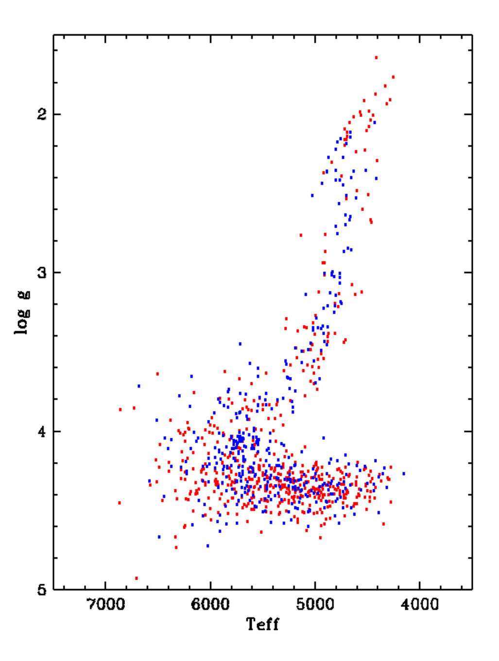
Then, in order to more precisely characterise the thick and thin disc populations previously defined, and to take into account of the natural increase of the abundance measurement errors for metal-poor star’s spectra (Recio-Blanco et al., 2014), we have defined a new sub-sample of objects, hereafter called e (c.f. Table 3). This new sub-sample contains all stars with errors smaller than 0.15 dex and 0.05 dex in and , respectively for -1 dex plus metal-poor stars (-1), with allowed errors as large as 0.2 dex in and 0.08 dex. The final sample is shown in Fig. 12 and contains 1 016 stars. A black line (based on the low density regions defined in Fig. 11) is plotted in Fig. 12 to identify the separation between the thick and thin disc sequences. Fig. 13 shows the Hertzsprung-Russel (HR) diagram of this selected sub-sample e. The red and blue points correspond to stars in the defined thin and thick disc sequences, respectively.
The thick disc sequence (filled circles in Fig. 12) seems to extend from dex and dex to about dex and dex, decreasing linearly with a slope of about -0.30. We have also considered metallicity bins of 0.2 dex and calculated the dispersion in for each bin. The resulting mean dispersion is 0.042 dex. This can be compared to the mean error in that is equal to 0.03 dex. On the other hand, the thin disc sequence (open circles), seems to be present from about dex and dex, to about dex and dex, decreasing with a slightly milder slope of about -0.20.
In addition, a high- metal-poor population is also visible in our data, well above the Galactic plane (see Sect. 5), and occupying a flat sequence from -1.0 dex down to the lowest sampled metallicities (filled triangles in Fig. 12). The mean value of these halo stars is around 0.35 dex. This high- metal-poor sequence could be identified with the classical high- halo sequence or, at least partially, with the metal-weak thick disc population (Ruchti et al., 2011; Kordopatis et al., 2013a, e.g.). Moreover, in the same metal-poor metallicity regime ( values lower than -0.9 dex), a metal-poor low- sequence seems to exist (asterisks in Fig. 12). After an individual inspection of these low- metal-poor stars spectra, most of them have signal-to-noise values higher than 25 in the HR10 setup, and have thus reliable and measurements. When only the lower error measurements are considered (stars with errors smaller than 0.05 dex in and 0.15 dex in and signal-to-noise ratio for the HR10 spectra higher than 20), the low- metal-poor stars represent about 10% of the observed stars with values lower than -0.9 dex. These stars could confirm the low- metal-poor halo stars first observed by Nissen & Schuster (2010), and also reported by Nissen & Schuster (2011), Schuster et al. (2012), Adibekyan et al. (2012) and Ishigaki et al. (2013). On the other hand, the possible link between those objects and the metal-weak thick disc population (Morrison et al., 1990; Carollo et al., 2010; Kordopatis et al., 2013b, e.g.) seems to be ruled out by their low ratios, as metal-weak thick disc stars are reported to have dex (Ruchti et al., 2011). As a complementary description of these stars, the individual element abundances of these stars are analysed in Mikolaitis et al. (2014, in preparation).
4.1 Comparison with literature studies

First of all, we have compared the spatial distribution of the analysed targets with that of previous spectroscopic studies of large numbers of disc stars, with available measurements of the ratio, as it is the case of the Lee et al. (2011b) and Adibekyan et al. (2012) analysis. We recall that the former is a low-resolution study of stars with Galactic radius in the range 710 kpc, and the latter is a high-resolution analysis of solar-neighbourhood stars, located at a maximum distance of about 600 pc from the Sun. Fig. 14 shows the location of the GES targets analysed in this paper (e sub-sample of Fig. 12), in vertical distance to the Galactic plane and radial cylindrical Galactic coordinate R. To understand how many of the targets are outside the solar neighbourhood, the points are colour coded by distance. All the objects with distances smaller than D600 pc from the Sun are plotted in red and those with larger distances in black. As expected from the photometric target selection, 90% of the stars are at distances larger than D600 pc from the Sun (i.e. much further than the Adibekyan et al. (2012) sample, comprised mainly of stars within 50 pc).
Regarding the thin to thick disc separation in the vs. plane, the above identified gap is in agreement with the separation seen in the Adibekyan et al. (2012) data. Fig. 12 shows the Adibekyan et al. (2012) division, as a red line with three segments, that can be compared to our proposed separation, in black. Both lines are compatible, with very small differences probably due to possible offsets in the abundance measurements between the GES analysis and the Adibekyan et al. (2012) one, or to a possible adjustment between the [M/H] and the [Fe/H] abundances. On the other hand, the Lee et al. (2011b) analysis proposes a division line with a shallower slope as illustrated by the blue solid line in Fig. 12. The two dashed lines indicate their dividing points for the thin and the thick disc stars to avoid the misclassification of stars. We see that the lower dashed line allows to select thin disc stars in fair agreement with both our selection and the Adibekyan et al. (2012) one. However, the upper dashed line excludes an important part of the thick disc sequence with intermediate and low values, even if a bias between our measurements and the Lee et al. (2011b) ones could exist. This could come mainly from the identification of the metal-rich part of thick disc, that would be more difficult to separate from the thin disc from low resolution data, due to the small differences in the values.
Furthermore, the difference of slope observed in our sample between the thin and the thick disc sequences seems in agreement with the Haywood et al. (2013) analysis of Adibekyan et al. (2012) data, that already points out an iron enrichment of the thin disc lower than the thick disc one.
Finally, concerning the metal-rich end of the thin disc, no -rich metal-rich stars are observed in our sample, nor in the Lee et al. (2011b) one, contrary to the results of Adibekyan et al. (2011) and Gazzano et al. (2013) and Boeche et al. (2013), restricted to, or predominantly in, smaller distances from the Sun. Furthermore, we note here that the number of stars with higher than -0.1 dex is rather small in our sample, compared to the previously mentioned nearby studies.
5 Distribution of distances to the Galactic plane
 |
 |
As already mentioned in the Introduction, the thin and the thick discs are characterised by different scale heights. In order to explore the transition between these two populations, keeping in mind their chemical separation in the vs. plane as described in the above section, we have analysed the distribution of the derived distances to the Galactic plane (from the absolute values of the Galactic Z coordinate) for the target stars.
The left panel of Fig. 15 shows a three-dimensional view of the distance to the Galactic plane, in the Z-axis, as a function of and , for the analysed stars (sub-sample e of Fig. 12). This illustration is complemented, in the right panel, with a grey scale-coded two-dimensional plot of the distribution of Z values in the vs. plane. The red line shows the separation between the thick and the thin discs sequences, defined in Sec. 4 (c.f. Fig. 12). We point out that the possible halo stars discussed in the previous section are not shown in Fig. 15, because of the low number of objects per bin.
Regarding the thick disc population, the mean distances to the Galactic plane seem to decrease along the sequence, from the metal-poor end to the metal-rich one:
- •
Z1.5 kpc at -0.9 dex and 0.280.40 dex
- •
Z1.2 kpc at -0.5 dex and 0.210.30 dex
- •
Z0.8 kpc at -0.3 dex and 0.120.25 dex.
Therefore, as the metallicity increases, the thick disc seems to lay in thinner and thinner layers. On the other hand, the distribution of vertical distances to the plane with respect to the Galactocentric radial distance is not perfectly homogeneous (c.f. Fig. 14). More particularly, our sample is dominated by stars further away from the galactic plane in the inner parts of the disc with respect to the typical heights probed in regions outside of the solar radius. Thus, different Z heights can be representative of different ranges in R, and, if there were significant metallicity variations with respect to R, this would manifest as a variation in metallicity with height. However, as later explained in Sec. 9.2, our data show a flat distribution of and with galactocentric radius for the thick disc. Therefore, the gradient of Z that appears along the thick disc sequence in the v.s. plane, for increasing values should be a real effect, not caused by sampling.
On the other hand, the thin disc sequence shows a quite constant value of the mean distances of its stars to the Galactic plane of Z0.5 kpc, from the metal-poor side ( -0.8 dex) to the metal-rich one ( 0.3 dex). Again, this conclusion should not be influenced by the spatial coverage of the studied sample, despite the fact that the thin disc has a metallicity gradient with respect to R (c.f. Sec. 9.2). This is because the thin disc Z range is fairly homogeneously covered at the full range of Galactocentric radius, and, in particular, the mean Z value of the stars in the thin disc sequence does not present any clear trend with R.
As a consequence of the above conclusions, the transition from the thick disc sequence to the thin disc one, in the vs. plane, implies a steeper change in the mean Z distances at [M/H] around -0.8 dex than around -0.3 dex. This coincides with the fact that the chemical separation between both sequences (by a gap or a lower density region) seems clearer in the metal poor regime than in the metal rich one.
Finally, we point out that, as expected, there is a correlation between the Z distances and the associated errors, with larger errors for stars that are further from the plane. More particularly, the stars in the metal-poor high-alpha end ([M/H] around -1.0 dex) have errors around 0.45 kpc, while at [M/H] around -0.7 dex the error is about 0.20 kpc for the thick disc stars and around 0.075 kpc for the thin disc. Nevertheless, while the stars that are further from the plane have larger absolute distance errors, the percent error is actually smaller, as indicated in Figures 6 and 7.
6 Distribution of rotational velocities


The distribution of the cylindrical rotational velocities, VΦ, in the vs. plane, is shown in Fig. 16. The rotational velocities of the stars located in the thick disc sequence have a mean value of V17616 km/s, and those in the thin disc have a mean V2086 km/s. In addition, for the thick disc, the VΦ values seem to progressively increase from the metal-poor -rich end (with V150 km/s) to the metal-rich -poor one (V190 km/s), reaching values close to the thin disc ones.
On the other hand, a correlation between rotational velocity and metallicity is observed for both the thin and the thick disc stars, although with opposite signs. In order to exploit the fact that both and are available for our sample, we have decided to analyse the correlation of rotational velocity taking into account both chemical abundance parameters. To this purpose, and as illustrated in Fig. 17, we have used the mean values of the rotational velocity, for different bins of 0.05 dex in and 0.20 dex in , to derive its dependence with metallicity. The chosen bin lengths are higher than the mean errors in and (0.03 dex and 0.08 dex, respectively), but they allow us to have a robust statistics per bin (a mean of 64 stars for the thin disc sequence and 34 stars for the thick disc one).
First, all the bins along the thin and thick disc sequences were considered. For the thin disc stars, we find a gradient of Galactic rotation with metallicity of -176 km dex-1. We have checked the possible influence of the large range of sounded galactocentric radius on the derived gradient, by splitting the sample in two: stars inwards (R) and outwards (R) of the solar radius. The resulting values of the gradient are -2013 and -229 km dex-1, suggesting that the derived slopes are not indirectly created by radial gradients in metallicity. For the thick disc population, we find a positive gradient of 4313 km s-1 dex-1. The derived values of the gradient for the thin and the thick disc are in very good agreement with the Lee et al. (2011b) analysis of SEGUE data (who find -22.61.6 km s-1 dex-1 for the thin disc and 45.81.8 km s-1 dex-1 for the thick disc) and with the Adibekyan et al. (2013) measurements in the solar neighbourhood (-16.83.7 km s-1 dex-1 for the thin disc and 41.918.1 km s-1 dex-1 for the thick disc). Our gradient for the thick disc is also in agreement with the measurements of Kordopatis et al. (2011, 45 ± 12 km s-1 dex-1) and Spagna et al. (2010), derived, respectively, from low resolution FLAMES spectroscopy and SDSS spectro-photometry, with no estimations of . It also confirms the disagreement with the SDSS result of Ivezić et al. (2008), based on photometric metallicities.
Second, to analyse if the V value depends on the considered bins of , we have derived the mean value of for each metallicity bin and divided the thick disc sample in two regimes:
- •
a high- sample with those bins corresponding to values higher than the mean for a given metallicity
- •
a low- sample with the bins corresponding to lower values than the mean.
The mean values of along the thick disc sequence dividing the above defined sub-samples, at each metallicity bin, are 0.35 dex at 1.0 dex, 0.30 dex at 0.85 dex, 0.25 dex at 0.65 dex, 0.20 dex at 0.45 dex and 0.15 dex at 0.25 dex. The corresponding derived V slopes are overplotted in Fig. 17. The gradient of rotation with metallicity seems to be steeper than the mean (649 km s-1 dex-1 instead of 4313 km s-1 dex-1) when the high- bins are considered. On the contrary, the value of V is lower than the mean one when it is determined from the low- bins (3010 km s-1 dex-1). Given that the dispersion is rather comparable to the measurement errors, the existence of a real intrinsic dispersion can not be concluded. Indeed, the described dependence of the V gradient with the considered bins could be the sign of a contamination of the thick disc stars from the thin disc ones in the lower part of the thick disc sequence. If this is correct, the steeper gradients derived from the high- bins could be more characteristics of the thick disc population than the previously published ones of about 4313 km s-1 dex-1. To test this possibility, we have also derived the value of the slope, using all the bins along the thick disc sequence with a mean error in lower than 0.04 dex. The resulting slope is 5619 km s-1 dex-1 instead of 4313 km s-1 dex-1, confirming that the slope seems steeper for higher quality data.
Finally, to analyse the direct influence of in the stellar rotation for thick disc stars, we have also derived the correlation between rotation and separate from . As shown in Fig. 18, VΦ and are highly anticorrelated (the Spearman’s coefficient value is -0.85, corresponding to 0.72% of the VΦ variance). In addition, the correlation rank between VΦ and is even more significant than the one between VΦ and (having a Spearman’s coefficient value of 0.73, that accounts for 0.53% of the VΦ variance).


Furthermore, we have checked how azimuthal velocity varies with vertical height for the thick disc sequence stars. Fig. 19 shows the mean VΦ value as a function of Z, in four bins of 0.5 kpc. The error bars indicate the standard error of the mean, in each bin. Clearly, the azimuthal velocity seems to decrease with height, in particular for Z values higher than about 1 kpc. As a consequence, this could explain why in situ samples of the thick disc can show a higher value of the thick disc lag (hence lower VΦ values) than the local surveys (Wyse et al., 2006, see for instance).
7 Distribution of azimuthal and vertical velocity dispersions
The stellar velocity dispersions can also be studied for the two chemically separated thin and thick disc sequences with our data. To this purpose, as low quality velocity determinations increase artificially the velocity dispersions, we have further restricted our analysis sub-sample, allowing only stars with errors in azimuthal and vertical velocity lower than 70 km/s. This value was found imposing a good balance between the statistical robustness and the allowed maximum error in velocity. This new restriction, in addition to those of sub-sample e presented in Table 3, leaves a data set of 645 stars, with a mean error in VΦ of 31 km/s.
Fig. 20 shows the distribution of the measured (not error free) azimuthal and vertical velocity dispersions ( and ) as a function of metallicity and distance to the Galactic plane. The error bars come from the standard error of the derived standard deviations. As expected, both velocity dispersions are higher for the thick disc sequence than for the thin disc one. The mean value of is 545 km/s for the thick disc and 403 km/s for the thin disc. Regarding , the mean values are 485 km/s for the thick disc sequence and 323 km/s for the thin disc one. As shown in the upper panels of Fig. 20, no significant dependencies of either or with metallicity or Z seem to be present in the data. Nevertheless, for the thick disc, the measurements suggest a possible increase of with distance to the Galactic plane that is not visible for . This conclusion seems strengthened by the increase of the uncertainty on the derived mean VΦ values as Z increases, as shown in Fig. 19. A possible decrease of with increasing metallicity could also be present for the thick disc. In addition, around -0.3 dex, the dispersion in the azimuthal velocity of the thick and the thin discs seem roughly the same, with a further decrease of for the metal rich end of the thin disc. This seems to be in agreement with the behaviour of the azimuthal velocity as a function of the metallicity, shown in Fig. 17 (see also Section 6). Moreover, the metal-poor side of the thin disc sequence, that presents higher rotation values, shows also a slightly lower azimuthal velocity dispersion.
On the other hand, we point out that our determinations of the velocity dispersions could be affected by the lack of stars at very low Z values (only 37 of the thin disc stars and 17 of the thick disc ones, included the first considered bin of vertical distance, are at abs(z)250 pc). This could explain the slightly higher values of dispersion found close to the Galactic plane with respect to other surveys like RAVE (Burnett, 2010, e.g.).
Finally, for the thick disc sequence, the azimuthal velocity dispersion seems to be of the order of the vertical velocity dispersion, within the error bars. In any case, the analysed data do not suggest, as predicted by Binney (2012), a smaller than the corresponding for the thick disc.
 |
 |
 |
 |
8 Orbital parameters
To calculate the orbital parameters of the stars in the sample we integrated orbits in a Galactic potential consisting of a Miyamoto & Nagai (1975) disc, a Hernquist (1990) bulge and a spherical logarithmic halo. Their characteristic parameters took the values and kpc, kpc for the disk, and kpc for the bulge, and km/s, and kpc for the halo. In particular, the eccentricities of the stars were defined as where () is the maximum (minimum) distance reached by the star in its orbit in the past 2 Gyr.
8.1 Eccentricity distribution


It is today widely accepted that the shape of the eccentricity distribution of the stellar orbits can provide important constraints on the formation mechanisms of the Galactic disc (Sales et al., 2009). Figure 21 shows the distribution of orbital eccentricities for the thin (red line) and the thick disc (blue line) chemically selected stars. As expected, the thin disc distribution is strongly peaked at a low eccentricity value of . On the other hand, the thick disc is significantly broader and its median eccentricity is around 0.3. Compared to previous determinations, such as those of Wilson et al. (2011), Lee et al. (2011b) and Kordopatis et al. (2011), the shape is flatter and does not decline as fast at high eccentricities, although because of the small number of stars, the significance of this may be questionable.
In order to evaluate the errors in the computed eccentricities, we have calculated the median, 25 and 75 percentile values of the eccentricity from all orbits starting from 100 realisations of the stars position and velocity, convolved with the errors. Assuming a Gaussian distribution, we have derived a value of the standard deviation for each stellar eccentricity. The mean value of the standard deviation depends slightly on the eccentricity itself, and its equal to 0.14 at eccentricity0.20 and 0.13 at eccentricity0.80.
Furthermore, Figure 22 presents the stellar orbital eccentricities as a function of metallicity for the thin and the thick disc sequences (lower and upper panels, respectively). On one hand, the thin disc sequence presents a very similar eccentricity distribution through its whole metallicity range, with a majority of low eccentric orbits. In addition, when only thin disc stars with a distance to the plane lower than 400 pc are considered (blue open circles in Fig. 22), most of the thin disc stars with higher eccentric orbits disappear. In addition, this high eccentricity tail of the thin disc suffers from a very low statistics and the relatively large errors in the derived eccentricities. On the other hand, the thick disc sequence seems to present highly eccentric orbits mainly in the metal-poor regime (0.6 dex). Additionally, the metal-rich part of the thick disc sequence shows very similar eccentricities to the thin disc one. A similar behaviour of the mean eccentricity distribution with metallicity has also been observed by Adibekyan et al. (2013) in the solar neighbourhood. Finally, the derived slopes of the eccentricity dependence on metallicity, e, are -0.1580.081 dex-1 for the thick disc and -0.0270.045 dex-1 for the thin disc. These values are also in agreement with those determined by Adibekyan et al. (2013) for the solar neighbourhood (-0.1840.078 dex-1 and -0.0230.015 dex-1 for the thick and the thin disc respectively).
8.2 Maximum height above the plane

We have also studied the distribution of maximum heights above the Galactic plane, Zmax, for the stars in the thick disc sequence. To this purpose, as shown in Fig. 23, we have plotted the normalized Zmax distribution for three different metallicity intervals. The associated error to Zmax was calculated through the above described procedure, already used for the eccentricity error, and it is of the order of 0.6 kpc.
As expected from the analysis of the mean distances to the Galactic plane in Sect. 5, the Zmax distribution seems to peak at lower values as the metallicity increases. Since we are working with a colour/magnitude selected sample, the quantification of a gradient would need correction for the volume sampled as a function of metallicity. Nevertheless, the observed Z and Zmax distributions seem to suggest a rather steep vertical metallicity gradient in the thick disk. On the other hand, Katz et al. (2011) found a low gradient of -0.0680.009 dex kpc-1, derived without a chemical selection of the thick disc in the vs. plane. On the other hand, Bilir et al. (2012) derived a value of the vertical metallicity gradient in the thick disc of -0.0340.003 dex kpc-1, from a kinematically selected sample of RAVE stars. Finally, Ruchti et al. (2011) found an iron abundance vertical gradient of -0.090.05 dex kpc-1 for metal poor thick disc stars.
9 Radial gradients in rotation, metallicity and

9.1 The thin disc rotational velocity behaviour with Galactocentric radius.
First of all, as illustrated in Fig. 24, we examined a possible dependence of VΦ with the Galactocentric radius for the thin disc. To this purpose, we have selected from the thin disc stars of sub-sample e those within a distance to the Galactic plane lower than 700 pc. We have also selected stars having errors in VΦ smaller than 40 km/s for 7R9 kpc, up to 60 km/s for 6R7 kpc and 9R10 kpc and 50 elsewhere. In addition, we have performed a 2- clipping around the mean values of VΦ in three metallicity intervals (-0.5 dex, -0.5-0.3 dex and -0.3 dex). The final sample contains 283 stars with a mean error in VΦ of 23 km/s and a mean error in R of 130 pc. Due to the survey selection function for this first GES iDR1 release, most of the thin disc targets near the Galactic plane are within 5R11 kpc, with very few objects in the outer parts of the disc. The resulting least squares fit of the data shows a flat behaviour of the rotational velocity (with a slope of 0.21.6 km s-1 kpc-1, where the uncertainty comes from the standard error of the slope). For comparison, literature estimations of the Galactic rotation curve from individual velocities of 70 Carbon stars by Demers & Battinelli (2007), from gas clouds using the terminal velocities of the HI and CO lines (Sofue et al., 2009) and from APOGEE data (Bovy et al., 2012a), find an approximately flat behaviour, as what is found for the rotational velocity with our data.
In addition, we have tested the possible effect of the VΦ correlation with metallicity (c.f. Sect. 6) on the derived VΦ vs. R relation. To this purpose, we have divided the above described sample in three sub-samples for different metallicity intervals: -0.5 dex, -0.5-0.3 dex and -0.3 dex (see Fig 24). Then, three values of the slope were derived for each of the sub-samples. For all these metallicity intervals, the rotational velocity stays flat within the error bar. Therefore, no measurable influence of the stellar rotation correlation with metallicity seems to exist in the thin disc, within the studied galactocentric distance range. In agreement with Fig. 17, the mean value of VΦ decreases with metallicity, in the three considered metallicity intervals. Finally, we have checked a possible trend of the VΦ dispersion with R in the examined sample, finding a flat with R in the range 7R10 kpc, for which the number of stars allows a robust enough measurement of the VΦ dispersion.

9.2 Radial abundance gradients
In order to derive the radial abundance gradients in the thin disc, we have used the sample of stars described in Section 7.1 and performed least square fits to the v.s. distribution and the v.s. distribution (c.f. Fig. 25). We find a negative gradient of -0.0580.008 dex kpc-1 for and a very small positive gradient of 0.0120.002 dex kpc-1 for the . As in the previous section, the uncertainties come from the standard error of the slope, derived by the least square linear regression.
The value of the metallicity gradient is a matter of debate, ranging from -0.06 to -0.1 dex kpc-1. Our measured value is therefore in agreement within the literature intervals, as the most recent studies using Cepheid stars (around -0.06 dex kpc-1, see Lemasle et al., 2013, and references therein22 2 Measured with iron abundances) and dwarfs stars in the Corot mission fields (Gazzano et al., 2013, -0.0530.011 dex kpc-1). Measurements based on HII regions33 3 Measured with oxygen, nitrogen, and sulphur abundances. range from -0.0460.009 dex kpc-1 to -0.0710.010 dex kpc-1 in the optical and -0.0410.009 dex kpc-1 to -0.0850.010 dex kpc-1 in the infrared (Rudolph et al., 2006). Our metallicity gradient estimation is also in agreement with the Cheng et al. (2012) analysis of SEGUE data, who find -0.14 dex kpc-1 for 0.15 kpcZ0.25, -0.082 dex kpc-1 for 0.25 kpcZ0.50, and -0.024 dex kpc-1 for 0.50 kpcZ1.0, selecting low stars in their sample. Finally, observations of open clusters find steeper gradients for the inner regions (Andreuzzi et al., 2011; Magrini et al., 2009, dex kpc-1 for R12 kpc, c.f.), than for the whole covered radial range (Andreuzzi et al., 2011; Carrera & Pancino, 2011, dex kpc-1,). In addition, it is worth noticing that the different above mentioned indicators trace the gradient at different times, and the issue of the gradient evolution with time is indeed still open.
On the other hand, the very small positive gradient in the abundance ratio seems not to be influenced by the cut in vertical distance to the Galactic plane, as its value does not change if the cut is done at 400 pc instead of 700 pc. This could be the case if a contamination by thick disc stars was affecting the radial gradient measurement. However, the presence of numerous metal-poor thin disc stars with 0.5 dex in our sample, influences the measurement, steepening the gradient, as those stars present high values of and dominate the outer regions. If real, this slightly positive gradient in could be in agreement with the measurements of Yong et al. (2005) and Carrera & Pancino (2011) for open clusters, Carney et al. (2005) for field giants, and Yong et al. (2006) for Cepheids, who report an enhancement of in the outer disc. In particular, the result for the Cepheids of Yong et al. (2006) comes from stars in the metal-poor regime (-1.0-0.3 dex). Nevertheless, the individual -element abundances of Cepheids reported by Luck & Lambert (2011) in the range 4-15 kpc are compatible with a rather small positive gradient in Mg/Fe, whereas Lemasle et al. (2013) report a SiFe gradient close to zero and a very small gradient in CaFe of 0.016 dex/kpc (assuming the well accepted metallicity gradient for Cepheids of -0.06 dex/kpc), close to their measurement errors.
Moreover, we have checked the influence of the data spatial distribution in the derived gradients. For that purpose, it is necessary to test the robustness of the two derived gradients on the inhomogeneity of the survey in the R and Z distribution. As already explained in Section 5, our total sample is dominated by stars further away from the galactic plane in the inner parts of the disc with respect to the typical heights probed in regions outside of the solar radius. However, thanks to the restriction of the thin disc sample to Z values smaller than 700 pc, the above mentioned correlation between Z and R practically dissapears: the mean distance to the Galactic plane is 450 pc at R6 kpc and 300 pc at R12 kpc. This small trend can not be responsible for the measured gradients in metallicity and , especially, after the chemical selection of the stars from the thin disc sequence of the vs. plane. In addition, in the case of the gradient, the small negative trend of Z with R excludes a higher spurious thick disc contamination in the outer regions with respect to the inner ones, as we would expect if the gradient was artificially created by a bad thin-thick disc separation in the outer regions. Therefore, as a consequence of the two gradients in and , the outer parts of the thin disc sounded by the present sample of GES data (up to 12 kpc) appear more metal-poor and, possibly, slightly richer in than the inner regions.

Finally, we have also analysed the radial abundance gradients in the thick disc population (c.f. Fig 26), selecting stars in the thick disc sequence of the vs. plane, with Z distances higher than 700 pc. The cut in Z limits the contamination by thin disc stars and possible problems with the inhomogeneus sampling in R and Z. The derived slopes, both for and for thick disc stars, are within the corresponding error bars (0.0060.008 dex and -0.0040.003 dex respectively). Therefore, our data suggest a flat distribution with galactocentric radius, both for and for thick disc stars. Our result for the gradient is in agreement with the Cheng et al. (2012) flat gradient for their selected high- stars from SEGUE data.
10 Summary and discussion
We have used the atmospheric parameters, abundance ratios and radial velocities, determined from the Gaia-ESO Survey GIRAFFE spectra of FGK-type stars (first nine months of observations), to present the kinematical and chemical characterisation of the observed stellar populations. First, we have chosen to identify the thin to thick disc separation in the v.s. plane, thanks to the presence of a low-density region in the number density distribution. This separation is in agreement with the recently proposed one by Adibekyan et al. (2013) from a sample of solar neighbourhood stars, and the ones observed before by Fuhrmann (2004), Reddy et al. (2006) and Bensby et al. (2007), among others.
Furthermore, we have studied the distribution of the distances to the Galactic plane, in the v.s. plane, with particular attention to the chemically defined thin and thick disc populations. Regarding the thick disc, our results show that the stars lay in progressively thinner layers along the sequence (as metallicity increases and decreases). This finding could be in agreement with the Haywood et al. (2013) proposal of a thick disc forming stars in thinner and thinner layers for 4-5 Gyrs, also predicted by the dissipational settling formation scenario of Burkert et al. (1992). Similarly, Bovy et al. (2012c) already pointed out the scenario of an evolution in gradually thinner layers (as suggested by the dependence of their scale height distribution on ), although no clear separation between the thin and the thick disc sequences appears in their data. In addition, the recent hydrodynamic simulations of Bird et al. (2013) and Stinson et al. (2013) also show discs in which the younger stars have progressively shorter vertical scale heights. On the other hand, the thin disc sequence presents a constant value of the mean distance to the Galactic plane at all metallicities. As a consequence, the thick to thin disc transition in Z values appears more abrupt in the low metallicity regime.
Concerning the kinematics, the mean rotational velocities found for the thick and the thin disc sequences are in agreement with the canonical ones (V17616 km/s and V2086 km/s). In addition, the mean Galactic rotation also seems to increase progressively along the thick disc sequence, as the metallicity increases. Our data also confirm the already observed correlations between VΦ and for the two discs. In the case of the thick disc sequence, the mean value of the VΦ/ is 4313 km s-1 dex-1, is in agreement with the previous findings of Lee et al. (2011b), Kordopatis et al. (2011) and Spagna et al. (2010). This would confirm the disagreement with the SDSS result of Ivezić et al. (2008), based on photometric metallicities. Moreover, we have explored the possible influence of contaminating stars from the thin disc in the analysis of the correlation. If only the stars with the higher values at each metallicity bin are considered, the derived VΦ/ is 649 km s-1 dex-1. As a consequence, this steeper value of the gradient, cleaned from the influence of possible thin disc contaminants could be more characteristic of the real correlation for the thick disc. For the thin disc, a negative gradient of VΦ/-176 km dex-1 is found. Consequently, the difference in the characteristic rotational velocities between the thin and the thick disc are again accentuated in the low metallicity regime, as for the mean distances to the Galactic plane. Furthermore, the analysis of the velocity dispersions for the chemically separated thin and thick disc stars confirms a higher dispersion for the thick disc population than for the thin disc one, as expected, for both VΦ and Vz. Further, the stars in the thick and the thin disc sequences present also different distributions of their stellar orbit eccentricities, with the thick disc stars presenting a broader distribution peaked at higher eccentricities than the thin disc one.
Finally, we have analysed the properties of the thin and thick discs as a function of the Galactocentric radius. For the thin disc, we estimate a flat behaviour of the thin disc rotational velocity, a metallicity gradient equal to -0.0580.008 dex kpc-1 and, a very small positive gradient. For the thick disc, no gradients in and are found.
The general picture emerging from our analysis is that of a thick disc that lays in progressively thinner and thinner layers as the metallicity increases and the decreases with time (until about dex and dex). During this settling process, the thick disc rotation increases progressively and, possibly, the azimuthal velocity dispersion decreases. No measurable metallicity or gradients with galactocentric distance seem to remain for the thick disc. At about dex, the mean characteristics of the thick disc in , vertical distance to the plane, rotation and rotational dispersion are in agreement with (or just slightly different than) that of the thin disc stars of the same metallicity, suggesting a possible connection between the two populations at a certain moment of the disc evolution. This is in agreement with the Haywood et al. (2013) scenario, in which the inner thin disk (R10kpc) inherited from the chemical conditions left at the end of the thick disk phase (the observed metal-rich end of the thick disc sequence in the vs. plane), some 8 Gyr ago. In their view, there may be an age gap in the star formation possibly causing the gap in enrichment, after which, star formation proceeds in a thin disk.
For the thin disc, no clear gradient of the mean vertical distance to the plane with the stellar metallicity is observed. On the contrary, the stars in the metal-poor thin disc sequence tail seem to have a mean Galactic rotation velocity higher than those in the metal-rich part. Moreover, if confirmed, the existence of a small positive gradient in with R leads to a thin disc that would be slightly more metal-poor and -rich in the outer parts. These two characteristics, similar to those of the metal-poor end of the thin disc sequence in the v.s. plane, would favour the picture, suggested by Haywood et al. (2013) and Haywood (2006), of this metal-poor thin disc being formed in the outer parts.
Contrary to the similarities between the thin and the thick discs around 0.3dex, the stars in the metal-poor overlapping regime are more clearly separated in their mean physical properties (chemistry, kinematics, possibly orbital eccentricities). This separation seems to be confirmed by the gap (or low-density region) in the vs. .
On the other hand, the tight bimodal distribution of at every value of poses severe constraints to models predictions. Recent attempts to define an age-metallicity relation for stars currently in the solar neighbourhood (Haywood et al., 2013; Mishenina et al., 2013, e.g.) hint at an evolutionary path in which a very wide range of ages corresponds to a single value. Haywood et al. (2013) results (c.f. their Fig. 8) show that at a value of about -0.5 dex stars have an age range of around 10 Gyr. On the other hand, the present work and other studies focussed in the solar neighbourhood (Adibekyan et al., 2013, e.g.) show that the distribution of at -0.5 dex appears narrowly bimodal, with two essentially unresolved but quite discrete values of being found. As a consequence, although stars with -0.5 dex formed over 10Gyr, they seem to be formed with only two values of Ṫhis is a quite remarkably severe constraint that can be analysed in the light of Galactic models in which radial migration (Sellwood & Binney, 2002; Schönrich & Binney, 2009c; Schönrich & Binney, 2009b; Roškar et al., 2008, e.g.), and churning, is a major factor.
Schönrich & Binney (2009b) claim that a bimodal, although continuous, distribution of can naturally come out as a consequence of the standard assumptions about star formation rates and metal enrichment, with no need to invoke breaks in the Galaxy’s star formation history or accretion events. However, the tightness of the well populated observed thick and thin disc sequences in the vs. plane, with possibly only two values of for a given metallicity, poses severe constraints.
If radial migration occurs, one can suppose an evolutionary path in which enrichment in the high- branch happened rapidly, up to metallicities close to 0.25 dex. This should occur across a large enough radial range of the proto-galactic disk. In fact, to preserve the tightness of the high- sequence, the stars should had formed in a narrow time interval from radially well-mixed interstellar medium (ISM) gas, through all the galactocentric radii which generated stars that are today at a given R (ex. in the solar neighbourhod). Then, to explain the low- sequence, one can postulate a significant gas accretion, reducing the disc ISM metallicity to, for instance, -0.6 dex. This should be followed by disc evolution in which large scale gas flows (as in fountains, c.f. Fraternali et al., 2013, and references therein) retain a tight - correlation, over the radial region which today populates the solar neighbourhood. In addition, this scenario should, somehow, also conciliate the higher rotation values observed in the metal-poor thin disc regime. Othewise, other possibility to explain the observed vs. distributions, is to suppose that strong radial migration in the sense of churning did not occure (Haywood et al., 2013, see also the discussion in).
Finally, this study also shows the importance of precise chemical abundance measurements to disentangle the stellar population puzzle of the Galactic disc. The stellar chemical patterns can guide the definition of useful stellar sub-samples to unveil the evolutionary paths in the disc formation history and to give clearer constraints to the models. Moreover, in the near future, the Gaia mission of the European Space Agency will allow precise distances and ages estimations for all the analysed stars. The results presented here, based only on the first months of the GES observations, confirm how crucial are today large high-resolution surveys outside the solar neighbourhood for our understanding of the Milky Way history.
Acknowledgements.
Based on data products from observations made with ESO Telescopes at the La Silla Paranal Observatory under programme ID 188.B-3002. The results presented here benefit from discussions held during the Gaia-ESO workshops and conferences supported by the ESF (European Science Foundation) through the GREAT Research Network Programme. A. Recio-Blanco, P. de Laverny and V. Hill acknowledge the the support of the French Agence Nationale de la Recherche, under contract ANR-2010-BLAN- 0508-01OTP, and the "Programme National de Cosmologie et Galaxies" (PNCG) of CNRS/INSU, France. This work was partly supported by the European Union FP7 programme through ERC grant number 320360 and by the Leverhulme Trust through grant RPG-2012-541. We acknowledge the support from INAF and Ministero dell’Istruzione, dell’ Universita’ e della Ricerca (MIUR) in the form of the grant "Premiale VLT 2012". A. Helmi acknowledges financial support from ERC-Starting Grant, nr. GALACTICA-240271. Finally, we are sincerely grateful to the extremely careful anonymous referee, who undoubtedly enhanced the value of this paper.References
- Abadi et al. (2003) Abadi, M. G., Navarro, J. F., Steinmetz, M., & Eke, V. R. 2003, ApJ, 597, 21
- Adibekyan et al. (2013) Adibekyan, V. Z., Figueira, P., Santos, N. C., et al. 2013, A&A, 554, A44
- Adibekyan et al. (2011) Adibekyan, V. Z., Santos, N. C., Sousa, S. G., & Israelian, G. 2011, A&A, 535, L11
- Adibekyan et al. (2012) Adibekyan, V. Z., Sousa, S. G., Santos, N. C., et al. 2012, A&A, 545, A32
- Allende Prieto et al. (2006) Allende Prieto, C., Beers, T. C., Wilhelm, R., et al. 2006, ApJ, 636, 804
- Andreuzzi et al. (2011) Andreuzzi, G., Bragaglia, A., Tosi, M., & Marconi, G. 2011, MNRAS, 412, 1265
- Bensby & Feltzing (2010) Bensby, T. & Feltzing, S. 2010, in IAU Symposium, Vol. 265, IAU Symposium, ed. K. Cunha, M. Spite, & B. Barbuy, 300–303
- Bensby et al. (2005) Bensby, T., Feltzing, S., Lundström, I., & Ilyin, I. 2005, A&A, 433, 185
- Bensby et al. (2007) Bensby, T., Zenn, A. R., Oey, M. S., & Feltzing, S. 2007, ApJ, 663, L13
- Bilir et al. (2012) Bilir, S., Karaali, S., Ak, S., et al. 2012, MNRAS, 421, 3362
- Binney (2012) Binney, J. 2012, MNRAS, 426, 1328
- Bird et al. (2013) Bird, J. C., Kazantzidis, S., Weinberg, D. H., et al. 2013, ApJ, 773, 43
- Boeche et al. (2013) Boeche, C., Chiappini, C., Minchev, I., et al. 2013, A&A, 553, A19
- Bonifacio et al. (2000) Bonifacio, P., Monai, S., & Beers, T. C. 2000, AJ, 120, 2065
- Bournaud et al. (2009) Bournaud, F., Elmegreen, B. G., & Martig, M. 2009, ApJ, 707, L1
- Bovy et al. (2012a) Bovy, J., Allende Prieto, C., Beers, T. C., et al. 2012a, ApJ, 759, 131
- Bovy et al. (2012b) Bovy, J., Rix, H.-W., & Hogg, D. W. 2012b, ApJ, 751, 131
- Bovy et al. (2012c) Bovy, J., Rix, H.-W., Liu, C., et al. 2012c, ApJ, 753, 148
- Brook et al. (2007) Brook, C., Richard, S., Kawata, D., Martel, H., & Gibson, B. K. 2007, ApJ, 658, 60
- Brook et al. (2004) Brook, C. B., Kawata, D., Gibson, B. K., & Freeman, K. C. 2004, ApJ, 612, 894
- Burkert et al. (1992) Burkert, A., Truran, J. W., & Hensler, G. 1992, ApJ, 391, 651
- Burnett (2010) Burnett, B. 2010, DPhil thesis, Oxford University
- Carney et al. (2005) Carney, B. W., Yong, D., Teixera de Almeida, M. L., & Seitzer, P. 2005, AJ, 130, 1111
- Carollo et al. (2010) Carollo, D., Beers, T. C., Chiba, M., et al. 2010, ApJ, 712, 692
- Carpenter (2001) Carpenter, J. M. 2001, AJ, 121, 2851
- Carrera & Pancino (2011) Carrera, R. & Pancino, E. 2011, A&A, 535, A30
- Casetti-Dinescu et al. (2011) Casetti-Dinescu, D. I., Girard, T. M., Korchagin, V. I., & van Altena, W. F. 2011, ApJ, 728, 7
- Cheng et al. (2012) Cheng, J. Y., Rockosi, C. M., Morrison, H. L., et al. 2012, ApJ, 752, 51
- de Laverny et al. (2012) de Laverny, P., Recio-Blanco, A., Worley, C. C., & Plez, B. 2012, A&A, 544, A126
- Demarque et al. (2004) Demarque, P., Woo, J.-H., Kim, Y.-C., & Yi, S. K. 2004, ApJS, 155, 667
- Demers & Battinelli (2007) Demers, S. & Battinelli, P. 2007, A&A, 473, 143
- Edvardsson et al. (1993) Edvardsson, B., Andersen, J., Gustafsson, B., et al. 1993, A&A, 275, 101
- Fraternali et al. (2013) Fraternali, F., Marasco, A., Marinacci, F., & Binney, J. 2013, ApJ, 764, L21
- Freeman & Bland-Hawthorn (2002) Freeman, K. & Bland-Hawthorn, J. 2002, ARA&A, 40, 487
- Fuhrmann (1998) Fuhrmann, K. 1998, A&A, 338, 161
- Fuhrmann (2004) Fuhrmann, K. 2004, Astronomische Nachrichten, 325, 3
- Fuhrmann (2008) Fuhrmann, K. 2008, MNRAS, 384, 173
- Gazzano et al. (2013) Gazzano, J.-C., Kordopatis, G., Deleuil, M., et al. 2013, A&A, 550, A125
- Gilmore et al. (2012) Gilmore, G., Randich, S., Asplund, M., et al. 2012, The Messenger, 147, 25
- Gilmore et al. (2014) Gilmore, G., Randich, S., & et al. 2014, A&A
- Gilmore & Reid (1983) Gilmore, G. & Reid, N. 1983, MNRAS, 202, 1025
- Grevesse et al. (2007) Grevesse, N., Asplund, M., & Sauval, A. J. 2007, Space Sci. Rev., 130, 105
- Gustafsson et al. (2008) Gustafsson, B., Edvardsson, B., Eriksson, K., et al. 2008, A&A, 486, 951
- Harris (1996) Harris, W. E. 1996, AJ, 112, 1487
- Haywood (2006) Haywood, M. 2006, MNRAS, 371, 1760
- Haywood et al. (2013) Haywood, M., Di Matteo, P., Lehnert, M., Katz, D., & Gomez, A. 2013, ArXiv e-prints
- Hernquist (1990) Hernquist, L. 1990, ApJ, 356, 359
- Ishigaki et al. (2013) Ishigaki, M. N., Aoki, W., & Chiba, M. 2013, ApJ, 771, 67
- Ivezić et al. (2008) Ivezić, Ž., Sesar, B., Jurić, M., et al. 2008, ApJ, 684, 287
- Jones & Wyse (1983) Jones, B. J. T. & Wyse, R. F. G. 1983, A&A, 120, 165
- Jurić et al. (2008) Jurić, M., Ivezić, Ž., Brooks, A., et al. 2008, ApJ, 673, 864
- Katz et al. (2011) Katz, D., Soubiran, C., Cayrel, R., et al. 2011, A&A, 525, A90
- Koposov (2014) Koposov, S. e. a. 2014, A&A
- Kordopatis et al. (2013a) Kordopatis, G., Gilmore, G., Wyse, R. F. G., et al. 2013a, MNRAS, 436, 3231
- Kordopatis et al. (2013b) Kordopatis, G., Hill, V., Irwin, M., et al. 2013b, A&A, 555, A12
- Kordopatis et al. (2011) Kordopatis, G., Recio-Blanco, A., de Laverny, P., et al. 2011, A&A, 535, A107
- Lee et al. (2011a) Lee, Y. S., Beers, T. C., Allende Prieto, C., et al. 2011a, AJ, 141, 90
- Lee et al. (2011b) Lee, Y. S., Beers, T. C., An, D., et al. 2011b, ApJ, 738, 187
- Lee et al. (2011c) Lee, Y. S., Beers, T. C., An, D., et al. 2011c, ApJ, 738, 187
- Lejeune et al. (1998) Lejeune, T., Cuisinier, F., & Buser, R. 1998, A&AS, 130, 65
- Lemasle et al. (2013) Lemasle, B., Francois, P., Genovali, K., et al. 2013, ArXiv e-prints
- Liu & van de Ven (2012) Liu, C. & van de Ven, G. 2012, MNRAS, 425, 2144
- Loebman et al. (2011) Loebman, S. R., Roškar, R., Debattista, V. P., et al. 2011, ApJ, 737, 8
- Luck & Lambert (2011) Luck, R. E. & Lambert, D. L. 2011, AJ, 142, 136
- Magrini et al. (2009) Magrini, L., Sestito, P., Randich, S., & Galli, D. 2009, A&A, 494, 95
- McCall (2004) McCall, M. L. 2004, AJ, 128, 2144
- Mikolaitis et al. (2014) Mikolaitis, A., Recio-Blanco, A., & et al. 2014, A&A
- Minchev & Famaey (2010) Minchev, I. & Famaey, B. 2010, ApJ, 722, 112
- Mishenina et al. (2013) Mishenina, T. V., Pignatari, M., Korotin, S. A., et al. 2013, A&A, 552, A128
- Misiriotis et al. (2006) Misiriotis, A., Xilouris, E. M., Papamastorakis, J., Boumis, P., & Goudis, C. D. 2006, A&A, 459, 113
- Miyamoto & Nagai (1975) Miyamoto, M. & Nagai, R. 1975, PASJ, 27, 533
- Morrison et al. (1990) Morrison, H. L., Flynn, C., & Freeman, K. C. 1990, AJ, 100, 1191
- Nissen & Schuster (2010) Nissen, P. E. & Schuster, W. J. 2010, A&A, 511, L10
- Nissen & Schuster (2011) Nissen, P. E. & Schuster, W. J. 2011, A&A, 530, A15
- Norris (1999) Norris, J. E. 1999, Ap&SS, 265, 213
- Prochaska et al. (2000) Prochaska, J. X., Naumov, S. O., Carney, B. W., McWilliam, A., & Wolfe, A. M. 2000, AJ, 120, 2513
- Quinn et al. (1993) Quinn, P. J., Hernquist, L., & Fullagar, D. P. 1993, ApJ, 403, 74
- Ramírez et al. (2013) Ramírez, I., Allende Prieto, C., & Lambert, D. L. 2013, ApJ, 764, 78
- Recio-Blanco et al. (2014) Recio-Blanco, A., Allende Prieto, C., & et al. 2014, A&A
- Recio-Blanco et al. (2006) Recio-Blanco, A., Bijaoui, A., & de Laverny, P. 2006, MNRAS, 370, 141
- Reddy et al. (2006) Reddy, B. E., Lambert, D. L., & Allende Prieto, C. 2006, MNRAS, 367, 1329
- Reid (1993) Reid, M. J. 1993, ARA&A, 31, 345
- Rix & Bovy (2013) Rix, H.-W. & Bovy, J. 2013, A&A Rev., 21, 61
- Roeser et al. (2010) Roeser, S., Demleitner, M., & Schilbach, E. 2010, AJ, 139, 2440
- Roškar et al. (2008) Roškar, R., Debattista, V. P., Quinn, T. R., Stinson, G. S., & Wadsley, J. 2008, ApJ, 684, L79
- Ruchti et al. (2011) Ruchti, G. R., Fulbright, J. P., Wyse, R. F. G., et al. 2011, ApJ, 737, 9
- Rudolph et al. (2006) Rudolph, A. L., Fich, M., Bell, G. R., et al. 2006, ApJS, 162, 346
- Sales et al. (2009) Sales, L. V., Helmi, A., Abadi, M. G., et al. 2009, MNRAS, 400, L61
- Schlegel et al. (1998a) Schlegel, D. J., Finkbeiner, D. P., & Davis, M. 1998a, ApJ, 500, 525
- Schlegel et al. (1998b) Schlegel, D. J., Finkbeiner, D. P., & Davis, M. 1998b, ApJ, 500, 525
- Schlesinger et al. (2012) Schlesinger, K. J., Johnson, J. A., Rockosi, C. M., et al. 2012, ApJ, 761, 160
- Schönrich & Binney (2009a) Schönrich, R. & Binney, J. 2009a, MNRAS, 396, 203
- Schönrich & Binney (2009b) Schönrich, R. & Binney, J. 2009b, MNRAS, 396, 203
- Schönrich & Binney (2009c) Schönrich, R. & Binney, J. 2009c, MNRAS, 399, 1145
- Schönrich et al. (2010) Schönrich, R., Binney, J., & Dehnen, W. 2010, MNRAS, 403, 1829
- Schuster et al. (2012) Schuster, W. J., Moreno, E., Nissen, P. E., & Pichardo, B. 2012, A&A, 538, A21
- Sellwood & Binney (2002) Sellwood, J. A. & Binney, J. J. 2002, MNRAS, 336, 785
- Smolinski et al. (2011) Smolinski, J. P., Lee, Y. S., Beers, T. C., et al. 2011, AJ, 141, 89
- Sofue et al. (2009) Sofue, Y., Honma, M., & Omodaka, T. 2009, PASJ, 61, 227
- Spagna et al. (2010) Spagna, A., Lattanzi, M. G., Re Fiorentin, P., & Smart, R. L. 2010, A&A, 510, L4
- Statler (1988) Statler, T. S. 1988, ApJ, 331, 71
- Stinson et al. (2013) Stinson, G. S., Bovy, J., Rix, H.-W., et al. 2013, MNRAS, 436, 625
- Valenti & Piskunov (1996) Valenti, J. A. & Piskunov, N. 1996, A&AS, 118, 595
- Villalobos & Helmi (2008) Villalobos, Á. & Helmi, A. 2008, MNRAS, 391, 1806
- Williams et al. (2013) Williams, M. E. K., Steinmetz, M., Binney, J., et al. 2013, ArXiv e-prints
- Wilson et al. (2011) Wilson, M. L., Helmi, A., Morrison, H. L., et al. 2011, MNRAS, 413, 2235
- Wyse & Gilmore (1995) Wyse, R. F. G. & Gilmore, G. 1995, AJ, 110, 2771
- Wyse et al. (2006) Wyse, R. F. G., Gilmore, G., Norris, J. E., et al. 2006, ApJ, 639, L13
- Yong et al. (2005) Yong, D., Carney, B. W., & Teixera de Almeida, M. L. 2005, AJ, 130, 597
- Yong et al. (2006) Yong, D., Carney, B. W., Teixera de Almeida, M. L., & Pohl, B. L. 2006, AJ, 131, 2256
- Yoshii (1982) Yoshii, Y. 1982, PASJ, 34, 365
- Zwitter et al. (2010) Zwitter, T., Matijevič, G., Breddels, M. A., et al. 2010, A&A, 522, A54