KCL-PH-TH/2014-11, LCTS/2014-11, CERN-PH-TH/2014-049
ACT-3-14, UMN-TH-3332/14, FTPI-MINN-14/10
Resurrecting Quadratic Inflation in No-Scale
Supergravity in Light of BICEP2
John Ellisa, Marcos A. G. Garcíab, Dimitri V. Nanopoulosc and Keith A. Oliveb
aTheoretical Particle Physics and Cosmology Group, Department of
Physics, King’s College London, London WC2R 2LS, United Kingdom;
Theory Division, CERN, CH-1211 Geneva 23,
Switzerland
bWilliam I. Fine Theoretical Physics Institute, School of Physics and Astronomy,
University of Minnesota, Minneapolis, MN 55455, USA
cGeorge P. and Cynthia W. Mitchell Institute for Fundamental Physics and Astronomy,
Texas A&M University, College Station, TX 77843, USA;
Astroparticle Physics Group, Houston Advanced Research Center (HARC), Mitchell Campus, Woodlands, TX 77381, USA;
Academy of Athens, Division of Natural Sciences,
28 Panepistimiou Avenue, Athens 10679, Greece
ABSTRACT
The magnitude of primordial tensor perturbations reported by the BICEP2 experiment is consistent with simple models of chaotic inflation driven by a single scalar field with a power-law potential , in contrast to the WMAP and Planck results, which favored models resembling the Starobinsky model if running of the scalar spectral index could be neglected. While models of inflation with a quadratic potential may be constructed in simple supergravity, these constructions are more challenging in no-scale supergravity. We discuss here how quadratic inflation can be accommodated within supergravity, focussing primarily on the no-scale case. We also argue that the quadratic inflaton may be identified with the supersymmetric partner of a singlet (right-handed) neutrino, whose subsequent decay could have generated the baryon asymmetry via leptogenesis.
March 2014
1 Introduction
The discovery of primordial tensor perturbations by the BICEP2 experiment [1] would be an important step in fundamental physics, if it is confirmed, since it would prove the existence of quantum gravitational radiation. The BICEP2 result would demonstrate simultaneously the reality of gravitational waves, whose existence had previously only been inferred indirectly from binary pulsars [2], and quantization of the gravitational field. The existence of such tensor perturbations is a generic prediction of inflationary cosmological models [3, 4, 5], and the BICEP2 result is strong evidence in favour of such models, the ‘smoking graviton’, as it were.
Moreover, different inflationary models predict different magnitudes for the tensor perturbations, and the BICEP2 measurement [1] of the tensor-to-scalar ratio discriminates powerfully between models, favouring those with a large energy density . As such, it disfavours strongly the Starobinsky proposal [6, 7, 8] and similar models, such as Higgs inflation [9] and some avatars of supergravity models [10, 11, 12, 13, 14, 15, 16, 17]. That said, the BICEP2 result is in some tension with previous experiments such as the WMAP [18] and Planck satellites [19], which established upper limits on and seemed to favour very small values. We are not qualified to comment on the relative merits of these different experiments, which may be reconciled if the scalar spectral index runs fast, but for the purposes of this paper we take at face value the BICEP2 measurement of [1] while retaining the measurements of the tilt in the scalar spectrum, , found by the previous experiments [18, 19], with which BICEP2 is consistent.
Planck and previous experiments were in some tension with the single-field power-law inflationary potentials of the form where is a generic mass parameter. Among models with , that might be related directly to models with fundamental scalar fields , models with provided the least poor fits to previous data. However, even such quadratic models were barely compatible with the Planck results at the 95% CL [19]. Quadratic models [20] are, in some sense, the simplest, since just such a single form of the potential could describe dynamics throughout the inflationary epoch and the subsequent field oscillations, unlike monomial potentials of the form , which would require modification at small in order to accommodate a particle interpretation. Moreover, there are motivated particle models that would yield a quadratic potential, e.g., for the scalar supersymmetric partner of a singlet (right-handed) neutrino in a Type-I seesaw model of neutrino masses [21]. Such a model would make direct contact with particle physics, and the decays of sneutrino inflatons could naturally yield a cosmological baryon asymmetry via leptogenesis. Such a scenario would be a step towards a physical model of inflation.
In this paper we first set the scene by revisiting simple slow-roll inflationary models based on single-field monomial potentials of the form in light of the BICEP2 result [1]. We derive and explore the validity of a general consistency condition on monomial models:
| (1) |
where is the number of e-folds of inflation. This consistency condition is comfortably satisfied for the value (after dust subtraction) indicated by BICEP2 [1], and the values and consistent with this and other experiments [18, 19]. The consistency condition (1) is independent of the monomial power index , but in the quadratic case one finds for that and , in perfect agreement with the data. On the other hand, an potential would have , as we discuss later.
Global supersymmetry accommodates very naturally [22] a single-field model, one example being the sneutrino model [21] mentioned above. However, one should embed such a model in the framework of supergravity [23]. The first attempt at constructing an inflationary model in supergravity proposed a generic form for the superpotential for a single inflaton [24], the simplest example being [25]. However, these models relied on an accidental cancellation between contributions to the inflaton mass [26]. Such cancellations are absent in generic supergravity models, which typically yield effective potentials with higher powers of the inflaton field [27, 4, 5]. These problems can be alleviated either by employing a shift symmetry in the inflaton direction [28] or through no-scale supergravity [29, 30, 31]. Since no-scale supergravity arises as the effective field theory of compactified string theory [32], and is an attractive framework for sub-Planckian physics [33], this is an appealing route towards embedding quadratic inflation in a more complete theory.
The bulk of this paper explores possibilities for obtaining a quadratic inflaton potential in the context of supergravity. After briefly reviewing models that invoke a shift symmetry, we turn our focus to no-scale supergravity models. We distinguish two classes of such models, which are differentiated by how the moduli in the theory obtain their vevs. We give an explicit example that incorporates supersymmetry breaking and a simple quadratic inflationary potential embedded in no-scale supergravity with a stabilized Kähler modulus.
2 Inflation with power-law potentials
2.1 General power-law potentials
We work in the slow-roll approximation [5], where the magnitude of the scalar density perturbations implies that
| (2) |
where is value of the effective inflationary potential and is a slow-roll parameter given by [5]
| (3) |
where, here and subsequently, the prime denotes a derivative with respect to the inflaton field , and corresponds to the reduced Planck mass, GeV. Other slow-roll parameters are [5]
| (4) |
CMB observables can be expressed as follows in terms of the slow-roll parameters:
| (5) | |||||
| (6) | |||||
| (7) |
In addition to the above expressions, we note the formula
| (8) |
for the number of e-folds of inflation between the initial and final values of the inflaton field . Within this framework, the BICEP2 measurement [1] (after subtraction of an estimated dust contribution) provides a first direct determination of and hence, via (2), a determination of the potential energy density during inflation: . The measurement of then implies that also . Clearly, these determinations are consistent with the slow-roll approximation.
As already mentioned, there is tension between the BICEP2 measurement of and the Planck upper limit, which could be alleviated if there were significant running of the scalar index: [1]. Since and are both , corresponding to and , such a magnitude of the scalar spectral index would require and hence . In this case, the variation in over a range is , which is difficult to reconcile with the estimate of from measurements of and , and indeed the slow-roll approximation in general. We therefore assume instead that the running of the spectral index is negligible, in which case the tension between BICEP2 and Planck cannot be alleviated.
We now consider the simplest possible class of single-field models of inflation, namely a monomial of the form . In this case, the slow-roll parameters have the expressions
| (9) |
corresponding to
| (10) |
where we have now suppressed the suffix in , and the number of e-folds is
| (11) |
if we assume that . These expressions yield one consistency condition that is independent of and , namely
| (12) |
as noted earlier. As also noted earlier, the 68% CL ranges indicated by BICEP2 and other experiments [1, 18, 19], , combined with the expected number of e-folds , satisfy comfortably the consistency relation (12). This is not the case for the Planck upper limit on if the scalar spectral index does not run, namely at the 68% CL.
2.2 Quadratic Inflation
Given the consistency of the single-field monomial potential with experiment, one may then ask what value of is favoured. The expressions (10, 11) can be used to derive two expressions for that are independent of , namely
| (13) |
which can be combined to yield (12). Inserting , and , we find the values
| (14) |
Clearly these are highly consistent with the quadratic case . The cases () cannot be excluded, whereas () is strongly disfavoured ** * Potentials with combinations of quadratic and quartic terms have also been considered recently in light of BICEP2: see [34].. However, since the and potentials are not bounded below for negative , they would certainly require modification in this region, as well as near in order to have a particle interpretation, so we disfavour them. We are therefore led to consider quadratic inflation in more detail.
In the case , the analysis of [21] showed that mass of the inflaton, GeV , and we see from (11) that one requires an initial field value , corresponding to . The small value of (or, equivalently, ) raises the usual problems of fine-tuning and naturalness in the presence of quadratic divergences in the quantum corrections to the effective field theory. This issue would not arise if the inflaton is embedded in a supersymmetric theory. We also note that, if one relaxes the monomial assumption, any contribution of the form would need to have . In a supersymmetric theory, , where is some Yukawa coupling. Both and would receive only logarithmic wave-function renormalization, so that small values are technically natural. Moreover, since the Yukawa coupling of the electron , the constraint on does not seem unreasonable in a supersymmetric model. These are among the reasons why we think that “inflation cries out for supersymmetry” [22]. Within this framework, we pointed out specifically that suitably small values of the density perturbations could be accommodated naturally.
Supersymmetrizing the potential is a first step in incorporating BICEP2-compatible inflation into a more complete physics model. A second step is to identify the inflaton with the scalar partner of a singlet (right-handed) neutrino in a Type-I seesaw model of neutrino masses [21]. In this case, the sneutrino inflaton decays directly into Standard Model Higgs bosons and leptons, and one-loop effects naturally generate a CP-violating lepton asymmetry. It was shown in [21] that there is a large range of parameters in which sphalerons then generate an acceptable cosmological baryon asymmetry †† † The large energy density during inflation indicated by BICEP2 tends to indicate a high reheating temperature, which would yield a high gravitino density, but this is not necessarily a problem if the gravitino mass is high enough - a possibility compatible with the specific inflationary supergravity scenarios discussed later.. Sneutrino inflation seems to us a very attractive scenario for linking early cosmology to particle physics in a testable way. In this scenario, requiring that lepton-number violation be absent would forbid any trilinear Yukawa interaction between neutrino superfields that could generate a quartic sneutrino coupling .
Within the Type-I seesaw model one is led naturally to consider the possibility that two or three sneutrinos might play rôles during the inflationary epoch [35]. It was found that they could, in general, decrease compared to the single-sneutrino model. This reduction would be accompanied by an increase in in a two-sneutrino model, but not necessarily in a three-sneutrino model. These possibilities illustrate the importance of detailed measurements of the tensor modes as well as refining the measurement of . A multi-sneutrino scenario could accommodate a value of intermediate between the values currently favoured by Planck and BICEP2. Another example capable of yielding an intermediate value of is the Wess-Zumino model [36], but we do not pursue these possibilities here.
3 Quadratic Inflation in Simple Supergravity
The scalar potential in supergravity is given by
| (15) |
where we can write in terms of a Kähler potential and superpotential
| (16) |
giving
| (17) |
where . The first attempt at chaotic inflation in supergravity was made in [37].
For generic Kähler potentials, the exponential prefactor typically leads to the -problem. An elegant mechanism for avoiding the -problem in supergravity with canonical kinetic terms employs a shift symmetry in the Kähler potential [28, 38, 39, 40, 41, 42, 43]‡‡ ‡ For recent limits on possible departures from shift symmetry, see [42]. Models of this type must incorporate at least two complex fields, three if one wants to incorporate supersymmetry breaking [41]. The general form of the Kähler potential should be , where the shift symmetry flattens the potential in the direction of the real part of . The simplest choice of Kähler potential is
| (18) |
which can be combined with a superpotential
| (19) |
to yield a simple form for the scalar potential:
| (20) |
It is clear that taking leads directly to the desired quadratic potential.
However, it is not immediately apparent how to embed the shift symmetry in a more fundamental framework, and the choice (19) of superpotential does not lend itself to a sneutrino interpretation of the inflaton §§ § For another approach to the -problem and sneutrino inflation in supergravity, see [44].. We are therefore led to consider other supergravity models that can yield quadratic inflation.
4 Quadratic Inflation in No-Scale Supergravity
We now consider how an effective potential of the form could be obtained in a no-scale supergravity framework [29], which is motivated by models of string compactification [32], and is hence a step towards an ultra-violet completion of the potential, as well as being an attractive framework for sub-Planckian physics [30, 33]. No-scale supergravity [29] incorporates an SU/SU U(1) symmetry leading to a Kähler potential of the form
| (21) |
where the complex field could be identified as a generic string modulus field that parameterizes, together with “matter” fields , an SU no-scale manifold [29, 30].
It is straightforward to show that we must incorporate such matter fields and consider . To see this, recall that the minimal no-scale SU(1, 1)/U(1) model may be written in terms of a single complex scalar field with the Kähler function
| (22) |
in which case the kinetic term becomes
| (23) |
and the effective potential becomes
| (24) |
There are no polynomial forms of that lead to a quadratic potential for a canonically-normalized field, and we are led to consider models with additional matter fields.
For our purposes here, we take and consider theories with just two complex fields. In this case, the no-scale Kähler potential may be written in the form
| (25) |
and the canonically-normalized fields can be taken as , , and .
4.1 Models with the Kähler Potential fixed dynamically
Within this general framework, one possibility is to fix the argument of the Kähler potential, in which case the scalar potential takes a form similar to that in a globally supersymmetric model, namely
| (26) |
where . It was assumed in [31] that some high-scale dynamics fixes the value of , and a superpotential was used, which yielded a potential of the form . This is a small-field inflation model that shares many of the same properties as the simple example mentioned earlier [25]. Unfortunately, both models predict and are now excluded by the Planck and other data [19, 1]. We also note that an early attempt at a chaotic inflation model in no-scale supergravity was made in [45], though this model suffers from an instability along the inflationary path [46].
On the other hand, a quadratic potential for the inflation is easily obtained from (26) by taking , again with the assumption that there is a fixed vev for . A more complete model of this type was considered in [47], which relied on a stabilizing field as in (18) and (19). This model provides for a vev for and leads to a quadratic potential for the inflaton. In fact, the superpotential can be taken exactly as in (19), namely , but with a Kähler potential
| (27) |
where . The corresponding potential has a minimum at . However, all these theories contain a nearly massless field associated with ¶¶ ¶ For related models, see [46]..
4.2 Models with the Kähler Potential undetermined
Alternatively, one may leave the argument of the Kähler potential undetermined, and consider instead the possibility that is fixed. Returning to the no-scale form for the Kähler potential given by Eq. (25), it was shown previously [10] that in this case a superpotential of the form
| (28) |
with from the amplitude of density fluctuations and reproduces the effective potential of the Starobinsky model [6], which is favoured by Planck data [19] but disfavoured by BICEP2 [1], under the assumptions that some ‘hard’ dynamics fixes the Kähler modulus :
| (29) |
where we assume henceforth that . An example of fixing was given in [11], and we return below with other examples of such strong stabilization. The model with the superpotential (28) is one of a class of no-scale models that yield Starobinsky-like inflationary potentials [11], but here we seek variants leading to a BICEP-2 compatible potential.
4.2.1 Models with the Inflaton identified with the Kähler Modulus
Within the no-scale framework, one is free to choose either or the modulus as the inflaton. One example of a superpotential for the latter option is [48]
| (30) |
where as before. It has recently been observed [49] that in this model Im has a quadratic potential when Re is fixed at the global minimum of the effective potential. Unfortunately, when Im , as would be required during inflation, the effective potential is minimized at a different value of Re , and the BICEP2-compatibility of the model is lost ∥∥ ∥ Fixing the value of is also an issue for this class of models: see [11] and the discussion below..
Inflationary evolution in this model is illustrated in Fig. 1, where we define
| (31) |
and assume that is set at its global minimum initially, , but assume a large initial value of and follow the evolution of and during inflation. We see in the top panel that quickly jumps to a value and then decreases gradually towards zero, exhibiting small oscillations at times in Planck units. Conversely, we see in the middle panel that relaxes rapidly to zero, exhibiting a small overshoot at a time in Planck units. Finally, we see in the bottom panel of Fig. 1 that most of the inflationary e-folds occur after has settled to zero, and are driven by the roll-down of . In this particular example, the number of e-folds is 60, set by our choice for the initial value of . However, the inflaton should be identified with , or equivalently , and it would be Starobinsky-like. We find the following values of the scalar tilt and the tensor-to-scalar ratio
| (32) |
We conclude that this model provides a Planck/WMAP-compatible model of inflation, but is not BICEP2-compatible. This problem of the original version of [49] was also noted in [50].


In a revised version of [49], it was shown that the problem outlined above and in [50] could be avoided by a modification of the Kähler potential adding a stabilization term of the type proposed originally in [51] and used more recently in [11]:
| (33) |
where, as an example, the case and was chosen. The introduction of this stabilization term leads to an acceptable potential in the direction, avoids the field evolution to large in the original version of [49] discussed above and in [50], and would seem to allow for the desired quadratic inflation. However, the introduction of this term leads to a severe instability in the direction, as can be seen in Fig. 2 where the scalar potential is shown in the , projection for the fixed values and .

This further problem can be cured with the inclusion of a second stabilization term in the Kähler potential (33):
| (34) |
where it is sufficient to take . The presence of the quartic term in in , forces to 0 [40, 41] and implements finally the desired quadratic inflation. The scalar potential of the model (30, 34) at is given by [49]
| (35) |
Its projection in the , plane is shown in Fig. 3, and the , projection for and is shown in Fig. 4. We note that a quadratic potential for results only when is fixed. Fortunately, at large , is driven to a -independent minimum at .

We display in Fig. 5 the evolutions of the four field components of the model (30, 34) during inflation. The normalization of the inflaton field defined in (31) differs from the canonical value by a numerical factor that is dependent on , as seen in its effective Lagrangian:
| (36) |
We note that at the coefficient of the kinetic term for is proportional to and thus the normalization of the kinetic term is positive for . Because of the non-canonical normalization, the initial value of in Fig. 5 must be larger than 15 in order to obtain e-folds. We also see in (36) that is related to the inflaton mass by a -dependent numerical factor. In the top panel of Fig. 5 we see that the inflaton falls smoothly towards zero and then exhibits characteristic oscillations. It is crucial that remain relatively fixed during the inflationary evolution so that the is driven by a quadratic potential. The second panel shows the evolution of , which is related in (31) to : it moves to its minimum at large and then begins oscillations, but does not modify the inflationary behaviour in an important way. For the choice , the minimum at large coincides with that at . The qualitative behavior of the solutions will not be affected by other choices of . The next two panels show the evolutions of and : they exhibit some damped oscillations before relaxing rapidly to zero. Finally, the bottom panel of Fig. 5 shows the growth of the number of e-folds during inflation. We find for the model (30, 34) the following values of the scalar tilt and the tensor-to-scalar ratio
| (37) |
We conclude that the model (30, 34) provides a satisfactory BICEP2-compatible model of inflation.


As a BICEP2-compatible alternative, we consider the following superpotential:
| (38) |
Since we seek to identify the inflaton with a component of the modulus field , we must postulate some suitable ‘hard’ dynamics to fix . We consider for this purpose a modification of the Kähler potential that is higher order in and similar to that proposed in [51, 11, 12]:
| (39) |
In this model the canonically-normalized inflaton field is given by
| (40) |
and it is easy to verify that the parameter in (38) can be identified as the mass of the inflaton. Indeed, at the global minimum of the effective scalar potential, the mass of the field is also .
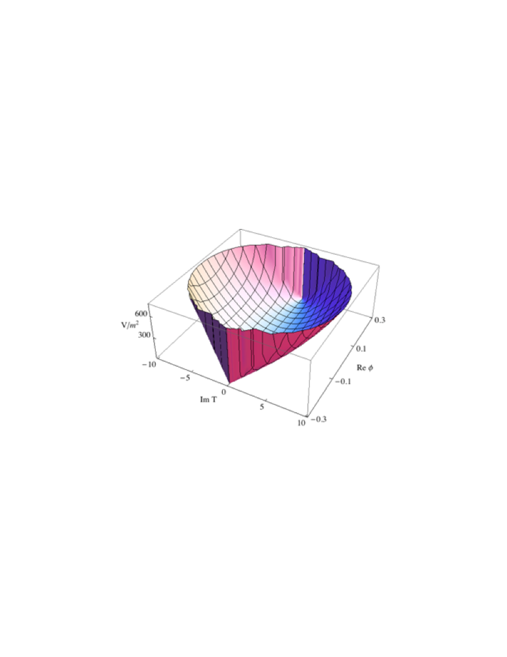
We display the effective scalar potential of the model (38, 39, 40) in various projections in Fig. 6, 7 and 8. Fig. 6 shows the effective potential for the real and imaginary components of . We see that both are stabilized around and, as already mentioned, the effective potential for has a BICEP2-compatible quadratic form. Fig. 7 shows that the modification (39) of the Kähler potential indeed fixes both components of . The range of is restricted by a singularity that appears as a near-vertical wall in Fig. 7. Finally, Fig. 8 shows the effective potential for the real parts of and . We conclude that this model provides a BICEP2-compatible model of inflation.


4.2.2 A Model with the Kähler Modulus fixed dynamically
As an alternative, we now investigate a model with the Kähler Modulus fixed dynamically and the inflaton identified with the other no-scale field, using a different choice of superpotential that yields an effective quadratic potential.
In such a no-scale scenario with fixed, the canonically-normalized inflaton field is defined by [10]
| (41) |
and the effective potential is
| (42) | |||||
| (43) |
Let us assume that inflation occurs along the real direction, . In the case of a quadratic potential, if . However, we see from (42) and (43) that, for a generic superpotential, the scalar potential grows exponentially fast at large :
| (44) |
The presence of the exponential is directly related to the presence of poles at , since for , . Therefore, if we are to have large-field inflation, one or both of the poles must be removed: . However, if this is the case, large implies , and for a polynomial superpotential , , corresponding to an asymptotically scale-invariant potential along the inflationary trajectory, more akin to the Starobinsky scenario than to the quadratic case.
It is possible to construct a quadratic potential if one relaxes the assumption for by allowing a non-polynomial form. Indeed, the choice
| (45) |
yields the effective potential , and it is clearly possible to construct alternative models that yield smaller values of . We note that the choice (45) has a symmetry: , consistent with the identification of the scalar component of as a sneutrino.
We also note that the imaginary direction of cannot support inflation for a general superpotential, due to the presence of singularities at Im . With the singularities removed, a superpotential that is polynomial in would result in a potential , with a range limited to Im .
4.3 A Modified No-Scale Model
As an alternative, one may consider the modified no-scale Kähler potential **** ** Such a form could appear if lies in a different modular sector, with the other modulus fixed by dynamics that we do discuss here.
| (46) |
The scalar field is now canonical, and in this case the scalar potential is of the form
| (47) |
assuming that the superpotential is a function of only and where we have again below set (see below for a mechanism which accomplishes this). It is then easy to see that the choice
| (48) |
again yields the effective potential , . In Eq. (48), the presence of the constant accounts for supersymmetry breaking with the gravitino mass given by . Therefore, we expect . The superpotential (48) also has the symmetry: , and is far simpler than the previous case (45), so we select it for more detailed study.
The model (46, 48) has two complex fields and hence four degrees of freedom. In order to show that this is a satisfactory model of inflation, one should demonstrate that the other degrees of freedom do not ‘misbehave’ while the real part of is driving inflation. We note first that the potential (47) given by (46, 48) is proportional to . Thus the potential rises exponentially along the Im direction, so that direction is automatically stabilized. In contrast, the potential given by (46, 48) is flat in the directions corresponding to the real and imaginary parts of , which must be stabilized in order to obtain suitable inflation. This can be achieved by modifying the Kähler potential to become [51, 11]
| (49) |
in which the quartic terms in the argument of the logarithm fix the vevs: and , providing the necessary stabilization. The masses of the real and imaginary parts of are both given by and thus are hierarchically larger than the gravitino mass. This type of hierarchy was recently shown to be compatible with preserving the baryon asymmetry while not over-producing the dark matter density through moduli and gravitino decays [52].
The shapes of the effective scalar potential in various projections are shown in Fig. 9, 10 and 11. We see explicitly in Fig. 9 the form of the effective potential for the real and imaginary components of , assuming that for the fixed value and . By construction, the real part of has the desired quadratic potential, and we see that the effective potential for the imaginary part has a minimum at . Secondly, Fig. 10 shows, correspondingly, that the real parts of and are indeed stabilized in the neighborhood of and . The curvature of the potential for the degree of freedom corresponding to is difficult to see in this figure, as its mass is in Planck units, which is hierarchically smaller than the mass of the inflaton , in this example. Thirdly, Fig. 11 shows, correspondingly, that both the real and imaginary parts of are indeed stabilized in the neighborhood of and when .


It is necessary also to verify also that the real and imaginary components of both and evolve correctly during the inflationary epoch. Accordingly, in Fig. 12 we display the evolutions of all four components during the inflationary epoch, assuming in (49), starting from the initial conditions
| (50) |
and assuming and . The top, second, third and fourth panels in Fig. 12 display the evolutions of and , respectively. We see that the inflaton evolves as expected towards zero, ending with some mild oscillations, and that there some harmless initial oscillations in , while the other field components remain very close to their values at the minimum of the effective potential throughout the inflationary epoch. The bottom panel of Fig. 12 displays the evolution of the cosmological scale factor during the inflationary epoch, demonstrating that a suitable number of e-folds can be obtained. The values of the scalar tilt and the tensor-to-scalar ratio are
| (51) |
We conclude that the model (49, 48) provides a satisfactory BICEP2-compatible model of inflation.


5 Summary and Conclusions
We have shown that the BICEP2 data on and the available data on are consistent (1) with a simple power-law, monomial, single-field model of inflation, and that is the power-law that best fits the available data (14). The required value of GeV and the small value of the quartic coupling required for the quadratic potential is to be a good approximation when during inflation are technically natural in a supersymmetric model [22]. Moreover, it is attractive to identify the inflaton with a singlet (right-handed) sneutrino, since this value of lies within the range favoured in Type-I seesaw models of neutrino masses. It is natural to embed quadratic (sneutrino) inflation within a supergravity framework, and we have given examples how this may be done in the context of both minimal and no-scale supergravity.
Nevertheless, we would like to reiterate that the BICEP2 measurement of is in tension with the Planck upper limit on , and emphasize that our choice here to discard the latter and explore the implications of the former is somewhat arbitrary. In our ignorance, we have no opinion how the tension between the two experiments will be resolved. If it is resolved in favour of Planck, Starobinsky-like models would return to favour, which can easily be accommodated in the no-scale supergravity framework, in particular, with a relatively simple superpotential such as (28). Alternatively, if the resolution favours BICEP2, as we have shown in this paper, the simplest possible potential would be favoured, which offers a very attractive connection to particle physics if the inflaton is identified as a sneutrino. As we have shown, such a model could also be accommodated within a no-scale supergravity framework, though at the expense of a more complicated superpotential such as (45) or (48). Models with values of intermediate between the ranges favoured by Planck and BICEP2 can also be constructed within the no-scale framework. A final caveat is that all our analysis is within the slow-roll inflationary paradigm, whereas the resolution of the tension between Planck and BICEP2 might require going beyond this framework, e.g., to accommodate large running of the scalar spectral index, a stimulating possibility that lies beyond the scope of this work.
Acknowledgements
The work of J.E. was supported in part by the London Centre for Terauniverse Studies (LCTS), using funding from the European Research Council via the Advanced Investigator Grant 267352. The work of D.V.N. was supported in part by the DOE grant DE-FG03-95-ER-40917 and would like to thank A.P. for inspiration. The work of M.A.G.G. and K.A.O. was supported in part by DOE grant DE-FG02-94-ER-40823 at the University of Minnesota.
References
- [1] P. A. R. Ade et al. [BICEP2 Collaboration], arXiv:1403.3985 [astro-ph.CO].
- [2] R. A. Hulse, J. H. Taylor, Ap. J. 195, L51 (1975).
- [3] K. A. Olive, Phys. Rept. 190 (1990) 307.
- [4] A. D. Linde, Particle Physics and Inflationary Cosmology (Harwood, Chur, Switzerland, 1990); D. H. Lyth and A. Riotto, Phys. Rep. 314 (1999) 1 [arXiv:hep-ph/9807278].
- [5] For a recent encyclopedic review see: J. Martin, C. Ringeval and V. Vennin, arXiv:1303.3787 [astro-ph.CO] and references therein.
- [6] A. A. Starobinsky, Phys. Lett. B 91, 99 (1980).
- [7] V. F. Mukhanov and G. V. Chibisov, JETP Lett. 33, 532 (1981) [Pisma Zh. Eksp. Teor. Fiz. 33, 549 (1981)].
- [8] A. A. Starobinsky, Sov. Astron. Lett. 9, 302 (1983).
- [9] F. Bezrukov and M. Shaposhnikov, JHEP 0907, 089 (2009) [arXiv:0904.1537 [hep-ph]].
- [10] J. Ellis, D. V. Nanopoulos and K. A. Olive, Phys. Rev. Lett. 111 (2013) 111301 [arXiv:1305.1247 [hep-th]];
- [11] J. Ellis, D. V. Nanopoulos and K. A. Olive, JCAP 1310 (2013) 009 [arXiv:1307.3537 [hep-th]];
- [12] R. Kallosh and A. Linde, JCAP 1306, 028 (2013) [arXiv:1306.3214 [hep-th]].
- [13] W. Buchmuller, V. Domcke and K. Kamada, Phys. Lett. B 726, 467 (2013) [arXiv:1306.3471 [hep-th]].
- [14] F. Farakos, A. Kehagias and A. Riotto, Nucl. Phys. B 876, 187 (2013) [arXiv:1307.1137].
- [15] S. Ferrara, R. Kallosh, A. Linde and M. Porrati, arXiv:1307.7696 [hep-th].
- [16] J. Ellis and N. E. Mavromatos, Phys. Rev. D 88 (2013) 085029 [arXiv:1308.1906 [hep-th]]; J. Alexandre, N. Houston and N. E. Mavromatos, Phys. Rev. D 89 (2014) 027703 [arXiv:1312.5197 [gr-qc]].
- [17] C. Pallis, arXiv:1312.3623 [hep-ph].
- [18] G. Hinshaw et al. [WMAP Collaboration], Astrophys. J. Suppl. 208, 19 (2013) [arXiv:1212.5226 [astro-ph.CO]].
- [19] P. A. R. Ade et al. [Planck Collaboration], arXiv:1303.5082 [astro-ph.CO].
- [20] A. D. Linde, Nucl. Phys. B 252, 153 (1985); M. S. Madsen and P. Coles, Nucl. Phys. B 298, 701 (1988).
- [21] H. Murayama, H. Suzuki, T. Yanagida and J.-i. Yokoyama, Phys. Rev. Lett. 70 (1993) 1912 and Phys. Rev. D 50 (1994) 2356 [hep-ph/9311326]; J. R. Ellis, M. Raidal and T. Yanagida, Phys. Lett. B 581 (2004) 9 [hep-ph/0303242].
- [22] J. R. Ellis, D. V. Nanopoulos, K. A. Olive and K. Tamvakis, Phys. Lett. B 118 (1982) 335; Phys. Lett. B 120 (1983) 331; Nucl. Phys. B 221 (1983) 52.
- [23] D. Z. Freedman, P. van Nieuwenhuizen and S. Ferrara, Phys. Rev. D 13 (1976) 3214; S. Deser and B. Zumino, Phys. Lett. B 62 (1976) 335.
- [24] D. V. Nanopoulos, K. A. Olive, M. Srednicki and K. Tamvakis, Phys. Lett. B 123, 41 (1983).
- [25] R. Holman, P. Ramond and G. G. Ross, Phys. Lett. B 137, 343 (1984).
- [26] A. D. Linde and A. Westphal, JCAP 0803, 005 (2008) [arXiv:0712.1610 [hep-th]].
- [27] E. J. Copeland, A. R. Liddle, D. H. Lyth, E. D. Stewart and D. Wands, Phys. Rev. D 49, 6410 (1994) [astro-ph/9401011]; E. D. Stewart, Phys. Rev. D 51, 6847 (1995) [hep-ph/9405389].
- [28] M. Kawasaki, M. Yamaguchi and T. Yanagida, Phys. Rev. Lett. 85, 3572 (2000) [arXiv:hep-ph/0004243].
- [29] E. Cremmer, S. Ferrara, C. Kounnas and D. V. Nanopoulos, Phys. Lett. B 133 (1983) 61; J. R. Ellis, A. B. Lahanas, D. V. Nanopoulos and K. Tamvakis, Phys. Lett. B 134 (1984) 429.
- [30] A. B. Lahanas and D. V. Nanopoulos, Phys. Rept. 145 (1987) 1.
- [31] J. R. Ellis, K. Enqvist, D. V. Nanopoulos, K. A. Olive and M. Srednicki, Phys. Lett. B 152 (1985) 175 [Erratum-ibid. 156B (1985) 452].
- [32] E. Witten, Phys. Lett. B 155 (1985) 151.
- [33] J. Ellis, A. Mustafayev and K. A. Olive, Eur. Phys. J. C 69, 219 (2010) [arXiv:1004.5399 [hep-ph]]; J. Ellis, D. V. Nanopoulos and K. A. Olive, Phys. Rev. D 89, 043502 (2014) [arXiv:1310.4770 [hep-ph]].
- [34] T. Kobayashi and O. Seto, arXiv:1403.5055 [astro-ph.CO]; X. Calmet and V. Sanz, arXiv:1403.5100 [hep-ph].
- [35] J. Ellis, M. Fairbairn and M. Sueiro, arXiv:1312.1353 [astro-ph.CO].
- [36] D. Croon, J. Ellis and N. E. Mavromatos, Physics Letters B 724 (2013) , 165 [arXiv:1303.6253 [astro-ph.CO]]; J. Ellis, N. E. Mavromatos and D. J. Mulryne, arXiv:1401.6078 [astro-ph.CO].
- [37] A. B. Goncharov and A. D. Linde, Phys. Lett. B 139, 27 (1984).
- [38] M. Yamaguchi and J. Yokoyama, Phys. Rev. D 63, 043506 (2001) [arXiv:hep-ph/0007021]; M. Yamaguchi, Phys. Rev. D 64, 063502 (2001) [arXiv:hep-ph/0103045]; M. Kawasaki and M. Yamaguchi, Phys. Rev. D 65, 103518 (2002) [arXiv:hep-ph/0112093]; M. Yamaguchi and J. Yokoyama, Phys. Rev. D 68 (2003) 123520 [arXiv:hep-ph/0307373]; P. Brax and J. Martin, Phys. Rev. D 72, 023518 (2005) [arXiv:hep-th/0504168]; K. Kadota and M. Yamaguchi, Phys. Rev. D 76, 103522 (2007) [arXiv:0706.2676 [hep-ph]]; F. Takahashi, Phys. Lett. B 693, 140 (2010) [arXiv:1006.2801 [hep-ph]]; K. Nakayama and F. Takahashi, JCAP 1011, 009 (2010) [arXiv:1008.2956 [hep-ph]]; K. Nakayama, F. Takahashi and T. T. Yanagida, Phys. Lett. B 725, 111 (2013) [arXiv:1303.7315 [hep-ph]].
- [39] S. C. Davis and M. Postma, JCAP 0803, 015 (2008) [arXiv:0801.4696 [hep-ph]].
- [40] R. Kallosh and A. Linde, JCAP 1011, 011 (2010) [arXiv:1008.3375 [hep-th]]; R. Kallosh, A. Linde and T. Rube, Phys. Rev. D 83, 043507 (2011) [arXiv:1011.5945 [hep-th]].
- [41] R. Kallosh, A. Linde, K. A. Olive and T. Rube, Phys. Rev. D 84, 083519 (2011) [arXiv:1106.6025 [hep-th]].
- [42] K. Harigaya and T. T. Yanagida, arXiv:1403.4729 [hep-ph].
- [43] K. Harigaya, M. Ibe, K. Schmitz and T. T. Yanagida, arXiv:1403.4536 [hep-ph]; K. Harigaya, M. Ibe, K. Ichikawa, K. Kaneta and S. Matsumoto, arXiv:1403.5880 [hep-ph].
- [44] S. Antusch, M. Bastero-Gil, K. Dutta, S. F. King and P. M. Kostka, JCAP 0901, 040 (2009) [arXiv:0808.2425 [hep-ph]].
- [45] A. S. Goncharov and A. D. Linde, Class. Quant. Grav. 1, L75 (1984).
- [46] H. Murayama, H. Suzuki, T. Yanagida and J. Yokoyama, Phys. Rev. D 50, 2356 (1994) [arXiv:hep-ph/9311326].
- [47] S. Antusch, M. Bastero-Gil, K. Dutta, S. F. King and P. M. Kostka, Phys. Lett. B 679, 428 (2009) [arXiv:0905.0905 [hep-th]].
- [48] S. Cecotti, Phys. Lett. B 190 (1987) 86.
- [49] S. Ferrara, A. Kehagias and A. Riotto, arXiv:1403.5531 [hep-th].
- [50] Z. Li, private communication; R. Kallosh, A. Linde, B. Vercnocke and W. Chemissany, arXiv:1403.7198 [hep-th]; K. Hamaguchi, T. Moroi and T. Terada, arXiv:1403.7521 [hep-ph].
- [51] J. R. Ellis, C. Kounnas and D. V. Nanopoulos, Phys. Lett. B 143, 410 (1984).
- [52] J. L. Evans, M. A. G. Garcia and K. A. Olive, arXiv:1311.0052 [hep-ph].