Generalized scale-invariant solutions to the two-dimensional stationary Navier-Stokes equations

We study a new special class of solutions to the stationary incompressible Navier-Stokes equations in $\Omega=\mathbb{R}^{2}\setminus\left\{\boldsymbol{0}\right\}$,

$\displaystyle\Delta\boldsymbol{u}-\boldsymbol{\nabla}p$

$\displaystyle=\boldsymbol{u}\boldsymbol{\cdot}\boldsymbol{\nabla}\boldsymbol{u}\,,$

$\displaystyle\boldsymbol{\nabla}\boldsymbol{\cdot}\boldsymbol{u}$

$\displaystyle=0\,,$

$\displaystyle\lim_{|\boldsymbol{x}|\to\infty}\boldsymbol{u}$

$\displaystyle=\boldsymbol{0}\,.$

(1)

An important parameter which labels the solutions of this system is the flux,

$$\Phi=\int_{\gamma}\boldsymbol{u}\boldsymbol{\cdot}\boldsymbol{n}\,,$$

(2)

which is independent of the choice of any simple closed curve $\gamma$ encircling the origin. The equations (1) are invariant under two types of symmetries: the rotations around the origin $\boldsymbol{u}(\boldsymbol{x})\mapsto\mathbf{R}^{-1}\boldsymbol{u}(\mathbf{R}\boldsymbol{x})$, with $\mathbf{R}\in\text{SO}(2)$ and the scaling $\boldsymbol{u}(\boldsymbol{x})\mapsto\lambda\boldsymbol{u}(\lambda\boldsymbol{x})$, with $\lambda\in\mathbb{R}$. The solutions that are invariant under these symmetries play a particular role (Wang, 1991, pp. 168-173) in the asymptotic behavior of the Navier-Stokes equations, as explained later. Šverák (2011) studied in details the scale-invariant solutions of the Navier-Stokes equations in dimension $d\geq 2$. In three dimensions, the only scale-invariant solutions are the Landau (1944) solutions, which decay like $\left|\boldsymbol{x}\right|^{-1}$ and are labeled by a vector in $\mathbb{R}^{3}$ whose norm determines the force acting on the fluid. In two-dimensions, Šverák (2011, §5) showed that the only scale-invariant solutions of (1) are the Hamel (1917, §6) solutions. The Hamel solutions are characterized by the flux $\Phi$ and a discrete parameter $n\in\mathbb{N}$, with an additional parameter $\mu$ for $n=0$. In polar coordinates $\left(r,\theta\right)$ they are given for $n=0$ by

$$\boldsymbol{u}_{\Phi,0}=\frac{\Phi}{2\pi r}\boldsymbol{e}_{r}+\frac{\mu}{r}\boldsymbol{e}_{\theta}\,,$$

(3)

where $\mu\in\mathbb{R}$ is an a additional parameter, and by

$$\boldsymbol{u}_{\Phi,n}=\frac{-1}{r}\varphi(\theta_{0}+\theta)\boldsymbol{e}_{r}\,,$$

(4)

for $n\in\mathbb{N}^{*}$ and $4+\frac{\Phi}{\pi}\leq n^{2}$, where $\varphi$ is a $\frac{2\pi}{n}$-periodic function determined by $n$ and $\Phi$, and $\theta_{0}$ is an angle that can be chosen arbitrarily. In view of their special form these solutions are scale-invariant, i.e. $\boldsymbol{u}(\boldsymbol{x})=\lambda\boldsymbol{u}(\lambda\boldsymbol{x})$. Moreover, it is interesting to note that in the case $n=0$, and $\Phi\neq-4\pi$, Hamel (1917, §11) found one more free parameter $A\in\mathbb{R}$ since

$$\boldsymbol{u}_{\Phi,0,A}=\frac{\Phi}{2\pi r}\boldsymbol{e}_{r}+\left(\frac{\mu}{r}+Ar^{1+\frac{\Phi}{2\pi}}\right)\boldsymbol{e}_{\theta}$$

(5)

is an exact solution of (1) provided $\Phi<-2\pi$. This solution in not scale-invariant and is bounded by $r^{-1}$ at infinity only for $\Phi\leq-4\pi$.

In what follows we look for solutions invariant under combinations of the scaling and rotational symmetries. We say that a solution $\boldsymbol{u}$ of the Navier-Stokes equations (1) is scale-invariant up to a rotation if there exists a rotation matrix $\mathbf{R}_{\lambda}\in\text{SO}(2)$ of continuously differentiable angle $R(\lambda)$ such that

$$\lambda\boldsymbol{u}(\lambda\boldsymbol{x})=\mathbf{R}_{\lambda}^{-1}\boldsymbol{u}(\mathbf{R}_{\lambda}\boldsymbol{x})\,,$$

(6)

for all $\lambda>0$. The scale-invariant solutions corresponds to the special case $R(\lambda)\equiv 0$. The aim of this paper is to determine all solutions of (1) that are scale-invariant up to a rotation, with $R(\lambda)$ a continuously differentiable function and discuss their implications.

Our main result is the following:

The study of scale-invariant solutions has proven to be of great importance, in particular for the determination of the asymptotic behavior of the stationary Navier-Stokes equations in two or three dimensions. The stationary and incompressible Navier-Stokes equations in the exterior domain $\Omega=\mathbb{R}^{2}\setminus B$ of a compact, connected set $B$ are

	$\displaystyle\Delta\boldsymbol{u}-\boldsymbol{\nabla}p$	$\displaystyle=\boldsymbol{u}\boldsymbol{\cdot}\boldsymbol{\nabla}\boldsymbol{u}\,,$	$\displaystyle\boldsymbol{\nabla}\boldsymbol{\cdot}\boldsymbol{u}$	$\displaystyle=0\,,$		(8a)
	$\displaystyle\left.\boldsymbol{u}\right|_{\partial B}$	$\displaystyle=\boldsymbol{u}^{*}\,,$	$\displaystyle\lim_{|\boldsymbol{x}|\to\infty}\boldsymbol{u}$	$\displaystyle=\boldsymbol{0}\,,$
where $\boldsymbol{u}^{*}$ is any smooth boundary condition with no net flux,
	$$\int_{\partial B}\boldsymbol{u}^{*}\boldsymbol{\cdot}\boldsymbol{n}=0\,.$$					(8b)

Problem (8b) is closely related to the one of the incompressible Navier-Stokes equations in $\mathbb{R}^{2}$,

$\displaystyle\Delta\boldsymbol{u}-\boldsymbol{\nabla}p$

$\displaystyle-\boldsymbol{u}\boldsymbol{\cdot}\boldsymbol{\nabla}\boldsymbol{u}=\boldsymbol{f}\,,$

$\displaystyle\boldsymbol{\nabla}\boldsymbol{\cdot}\boldsymbol{u}$

$\displaystyle=0\,,$

$\displaystyle\lim_{|\boldsymbol{x}|\to\infty}\boldsymbol{u}$

$\displaystyle=\boldsymbol{0}\,,$

(9)

where $\boldsymbol{f}$ is a smooth function of compact support. We remark, that the problems (8b) and (9) are very similar on a formal level: any solution of (8b) defines a solution of (9) on the exterior of the support of $\boldsymbol{f}$, and conversely any solution of (8b) can be truncated in order to obtain a solution of (9). In three dimensions, Nazarov & Pileckas (1999); Nazarov & Pileckas (2000) proved that the asymptotic behavior of solutions of (8b) is a scale-invariant solution. Then Korolev & Šverák (2011) simplified the proof by showing directly that, in this case, the Landau solution is the correct asymptotic behavior of any solution bounded by $\left(1+\left|\boldsymbol{x}\right|\right)^{-1}$. In two dimensions, existence of solutions to (8b) or (9) are not known in general (Galdi, 2004; Guillod & Wittwer, 2013), even for small data. The difference between two and three dimensions is essentially that in three dimensions the compatibility condition of the Stokes approximation to decay faster than $r^{-1}$ at infinity corresponds to the force and can be lifted by the Landau solutions which are exact solution of (9) with $\boldsymbol{f}(\boldsymbol{x})=\boldsymbol{b}\delta(\boldsymbol{x})$ where $\boldsymbol{b}\in\mathbb{R}^{3}$ is the net force and $\delta$ is the Dirac distribution. In two dimensions and in the case where $\boldsymbol{f}$ has non-zero mean, Guillod & Wittwer (2013) showed by physical arguments and detailed numerical verification that the velocity has to decay like $r^{-1/3}$ at infinity. In the case where $\boldsymbol{f}$ has zero mean, one would guess by analogy with the three-dimensional case that the asymptotic behavior should be a scale-invariant solution. However, Šverák (2011, §5) shows that one can not prove this by using perturbation techniques based on the Stokes approximation, and even together with the newly discovered solutions, we do not appear to be able to parameterize the general asymptotic behavior in the case where $\boldsymbol{f}$ has zero mean. The intuitive reason for this is the fact that the Stokes approximation has two compatibility conditions if we require the solution to decay faster than $r^{-1}$ at infinity: one of them might be lifted by adjusting the parameter $a$ of the new solutions, but we do not have sufficient parameters to lift also the other compatibility condition. We believe that the newly discovered solutions are a special case of a more general family of solutions, yet to be discovered, with one more parameter, corresponding to the general asymptotic behavior in the case where $\boldsymbol{f}$ has zero mean.

The paper in organized as follow. We first prove that the solutions which are scale-invariant up to a rotation are given explicitly in term of a $2\pi$-periodic function $\varphi$ satisfying an ordinary differential equation, and then we solve this differential equation by using elliptic functions. Finally we represent the solutions graphically, analyze the solutions having small amplitude, and discuss the implications for the solutions of Navier-Stokes equations.

We consider a solution $\boldsymbol{u}$ which is scale-invariant up to a rotation as defined in (6). In polar coordinates $\left(r,\theta\right)$ this symmetry is more easily expressed,

$\displaystyle\lambda u_{r}(\lambda r,\theta)$

$\displaystyle=u_{r}(r,\theta-R(\lambda))\,,$

$\displaystyle\lambda u_{\theta}(\lambda r,\theta)$

$\displaystyle=u_{\theta}(r,\theta-R(\lambda))\,.$

Therefore, by setting $\lambda=r^{-1}$, $u_{r}$ and $u_{\theta}$ are characterized by their values on $S^{1}$,

$\displaystyle u_{r}(r,\theta)$

$\displaystyle=\frac{1}{r}\varphi_{r}(\theta+R(r^{-1}))\,,$

$\displaystyle u_{\theta}(r,\theta)$

$\displaystyle=\frac{1}{r}\varphi_{\theta}(\theta+R(r^{-1}))\,,$

where $\varphi_{i}(\theta)=u_{i}(1,\theta)$ for $i\in\left\{r,\theta\right\}$. The divergence of the vector field $\boldsymbol{u}=u_{r}\boldsymbol{e}_{r}+u_{\theta}\boldsymbol{e}_{\theta}$ is

$$\boldsymbol{\nabla}\boldsymbol{\cdot}\boldsymbol{u}=\frac{1}{r^{2}}\left[\varphi_{\theta}^{\prime}(z)-r^{-1}R^{\prime}(r^{-1})\varphi_{r}^{\prime}(z)\right]\,,$$

where $z=\theta+R(r^{-1})$. The requirement of $\boldsymbol{u}$ to be divergence free therefore implies that

$\displaystyle R(\lambda)$

$\displaystyle=\theta_{0}-a\log\lambda\,,$

$\displaystyle\varphi_{\theta}(z)$

$\displaystyle=\mu-a\varphi_{r}(z)\,,$

where $a$, $\theta_{0}$ and $\mu$ are real constants. Consequently, a divergence free vector field satisfies the symmetry (6), if and only if $R(\lambda)=\theta_{0}-a\log\lambda$, and if it has the form

$\displaystyle\boldsymbol{u}$

$\displaystyle=\frac{1}{r}\left[-\varphi(z)\boldsymbol{e}_{r}+\left(\mu+a\varphi(z)\right)\boldsymbol{e}_{\theta}\right]\,,$

$\displaystyle z$

$\displaystyle=\theta_{0}+\theta+a\log r\,,$

(10)

where $\varphi$ is a $2\pi$-periodic function. The corresponding stream function $\psi$, defined such that $\boldsymbol{u}=\boldsymbol{\nabla}\boldsymbol{\wedge}\psi$, is

$$\psi(r,\theta)=\mu\log r+\Gamma(z)\,,$$

where $\Gamma$ is an antiderivative of $\varphi$.

We now determine the ordinary differential equation which $\varphi$ has to satisfy in order for $\boldsymbol{u}$ to be an exact solution of (1). The vorticity is

$$\omega=\frac{1+a^{2}}{r^{2}}\varphi^{\prime}(z)\,,$$

and the vorticity equation

$$\Delta\omega=\boldsymbol{u}\boldsymbol{\cdot}\boldsymbol{\nabla}\omega$$

becomes, after an explicit integration, the following ordinary differential equation

$$\left(1+a^{2}\right)\varphi^{\prime\prime}(z)-\left(\mu+4a\right)\varphi^{\prime}(z)+4\varphi(z)=\varphi(z)^{2}-C\,,$$

(11)

where $C\in\mathbb{R}$ is a constant related to certain averages of $\varphi$. By integrating the Navier-Stokes equations we can construct the pressure,

$$p=\frac{1}{r^{2}}\left[a\left(1+a^{2}\right)\varphi^{\prime}(z)-\left(2\left(1+a^{2}\right)+a\mu\right)\varphi(z)\right]-\frac{1}{2r^{2}}\left[\mu^{2}+C\left(1+a^{2}\right)\right]\,.$$

(12)

This shows that the only solutions of (1) which are scale-invariant up to a rotation are given by (10) and (12) where $\varphi$ is a $2\pi$-periodic function satisfying (11). The differential equation (11) is analog to the one describing the motion of a particle in a potential undergoing friction, and in order to obtain periodic solutions, the damping term has to vanish, i.e. $\mu+4a=0$. So we finally end up with a differential equation with two parameters: $a$ and $C$. In the next section we find the periodic solutions of this differential equation.

The ordinary differential equation (11) is clearly invariant under the translation $z\mapsto z+\theta_{0}$, so we do not keep track of this trivial symmetry and fix the origin later on in a convenient way. The trivial solutions where $\varphi$ is constant are not included in this analysis, since they correspond to the Hamel solutions (3). As explained above, in order to obtain periodic solutions we have to take $\mu+4a=0$, and therefore the ordinary differential equation (11) can be written as the differential equation describing a free particle in a potential,

$\displaystyle\varphi^{\prime\prime}$

$\displaystyle=-V^{\prime}(\varphi)\,,$

$\displaystyle V(\varphi)$

$\displaystyle=\frac{1}{1+a^{2}}\left[C\varphi+2\varphi^{2}-\frac{\varphi^{3}}{3}\right]\,.$

Finding the solutions of such an equation is rather standard (Rosenhead, 1940; Šverák, 2011, Theorem 2). The energy is conserved so

$\displaystyle E$

$\displaystyle=\frac{1}{2}\left(\varphi^{\prime}\right)^{2}+V(\varphi)\,,$

$\displaystyle\varphi^{\prime}$

$\displaystyle=\pm\sqrt{2E-2V(\varphi)}\,.$

Since we look for non-trivial periodic solutions, the potential has to have a minimum, so $C>-4$, and the energy has to be between the maximum and the minimum admissible values,

$$\frac{2}{3}\left(\sqrt{C+4}-2\right)\left(\sqrt{C+4}-2-C\right)<\left(1+a^{2}\right)E<\frac{2}{3}\left(\sqrt{C+4}+2\right)\left(\sqrt{C+4}+2+C\right)\,.$$

These two conditions imply that the polynomial $2E-2V(\varphi)$ has three distinct real roots, $\varphi_{1}<\varphi_{2}<\varphi_{3}$, and by Vieta’s formulas,

$$\varphi_{1}+\varphi_{2}+\varphi_{3}=6\,.$$

(13)

Therefore,

$$2E-2V(\varphi)=\frac{2}{3\left(1+a^{2}\right)}\left(\varphi-\varphi_{1}\right)\left(\varphi-\varphi_{2}\right)\left(\varphi-\varphi_{3}\right)\,,$$

and the solution is given in term of the incomplete elliptic function of the first kind $F$,

$$z(\varphi)=\sqrt{\frac{3}{2}}\sqrt{1+a^{2}}\int_{\varphi_{1}}^{\varphi}\frac{\mathrm{d}\varphi}{\sqrt{\left(\varphi-\varphi_{1}\right)\left(\varphi-\varphi_{2}\right)\left(\varphi-\varphi_{3}\right)}}=\sqrt{6}\frac{\sqrt{1+a^{2}}}{\sqrt{\varphi_{3}-\varphi_{1}}}F\left(\sqrt{\frac{\varphi-\varphi_{1}}{\varphi_{2}-\varphi_{1}}};\alpha\right)\,,$$

where

$$\alpha=\sqrt{\frac{\varphi_{2}-\varphi_{1}}{\varphi_{3}-\varphi_{1}}}\,.$$

We take the following convention for the elliptic integral $F$ (Gradshteyn & Ryzhik, 2007, §8.1),

$$F(x;\alpha)=\int_{0}^{x}\frac{\mathrm{d}t}{\sqrt{\left(1-t^{2}\right)\left(1-\alpha^{2}t^{2}\right)}}=\int_{0}^{\arcsin x}\frac{\mathrm{d}\theta}{\sqrt{1-\alpha^{2}\sin^{2}\theta}}\,.$$

The function $\varphi$ is $2\pi$-periodic if there exists $n\in\mathbb{N}^{*}$ such that

$$z(\varphi_{2})=\frac{\pi}{n}\,,$$

i.e., explicitly,

$$\frac{2\sqrt{1+a^{2}}K(\alpha)}{\sqrt{\varphi_{3}-\varphi_{1}}}=\sqrt{\frac{2}{3}}\frac{\pi}{n}\,,$$

(14)

where $K$ is the complete elliptic function of the first kind. The flux is given by

$$\Phi=\int_{\partial\Omega}\boldsymbol{u}\boldsymbol{\cdot}\boldsymbol{n}=\int_{\partial B(\boldsymbol{0},1)}\boldsymbol{u}\boldsymbol{\cdot}\boldsymbol{e}_{r}=-\int_{-\pi}^{+\pi}\varphi(z)\,\mathrm{d}z=-2n\int_{0}^{\pi/n}\varphi(z)\,\mathrm{d}z\,,$$

and, explicitly, by using the complete elliptic function of the second kind $E$,

$$\Phi=-n\sqrt{6}\int_{\varphi_{1}}^{\varphi_{2}}\frac{\sqrt{1+a^{2}}\,\varphi\,\mathrm{d}\varphi}{\sqrt{\left(\varphi-\varphi_{1}\right)\left(\varphi-\varphi_{2}\right)\left(\varphi-\varphi_{3}\right)}}=-2\sqrt{6}n\frac{\sqrt{1+a^{2}}}{\sqrt{\varphi_{3}-\varphi_{1}}}\left[\varphi_{3}K(\alpha)-\left(\varphi_{3}-\varphi_{1}\right)E(\alpha)\right]\,.$$

(15)

The conditions (13), (14) and (15) reduce to

$\displaystyle H(\alpha)$

$\displaystyle=\frac{1}{n^{2}\left(1+a^{2}\right)}\left(\pi^{2}+\frac{\pi\Phi}{4}\right)\,,$

$\displaystyle H(\alpha)$

$\displaystyle=\left[\left(\alpha^{2}-2\right)K(\alpha)+3E(\alpha)\right]K(\alpha)\,.$

(16)

Since the function $H$ is monotonic for $\alpha>0$ and its image is $\left(-\infty,\frac{\pi^{2}}{4}\right]$, this equation has a unique solution $\alpha_{n}>0$ for each $n\in\mathbb{N}^{*}$ satisfying

$$\frac{4+\frac{\Phi}{\pi}}{1+a^{2}}\leq n^{2}\,.$$

(17)

Since the equation determining $\alpha$ is continuous with respect to $a$ and $\Phi$, the solution $\varphi$ depends continuously on $a$ and $\Phi$ inside the region defined by (17).

For $n\in\mathbb{N}^{*}$, the exact solution $\boldsymbol{u}_{\Phi,n,a}$ exists provided condition (17) is satisfied. The corresponding region in the plane $\left(a,\Phi\right)$ is represented in figure 1. Moreover, for $n=0$, the Hamel solution $\boldsymbol{u}_{\Phi,0,A}$ defined by (5) with $A\neq 0$ exists for $\Phi<-2\pi$ and decays like $r^{-1}$ at infinity if $\Phi\leq-4\pi$, and less rapidly if $-4\pi<\Phi<-2\pi$. The linearization of the Navier-Stokes equations around the harmonic function (3) with $\mu=-4a$, can be solved exactly by the use of a Fourier series (Hillairet & Wittwer, 2013). The Fourier modes which are not zero decay faster than $r^{-1}$ provided a condition on $\Phi$ and $\mu$ holds. This condition is represented in figure 1 by a red curve, so that for all values above the curve the Fourier modes decay faster than $r^{-1}$ at infinity. The zero-flux case, was treated by Hillairet & Wittwer (2013), and they found that provided $\left|a\right|>\sqrt{3}$, the Navier-Stokes equations in the exterior of a unit disk with a Dirichlet boundary condition sufficiently close to $-4a\boldsymbol{e}_{\theta}$ admits a solution whose asymptote in given by $-4\tilde{a}\boldsymbol{e}_{\theta}/r$ where $\tilde{a}$ is close to $a$.

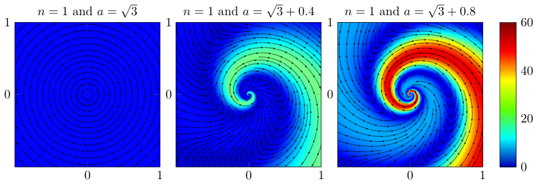
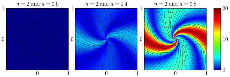
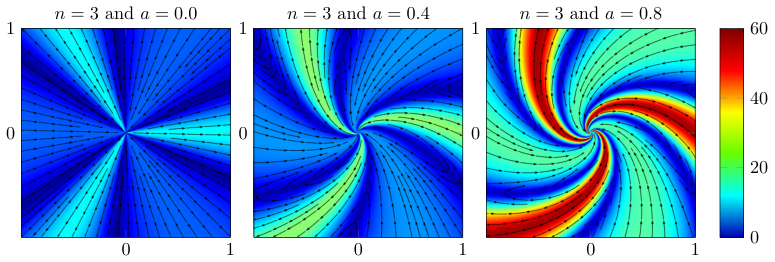
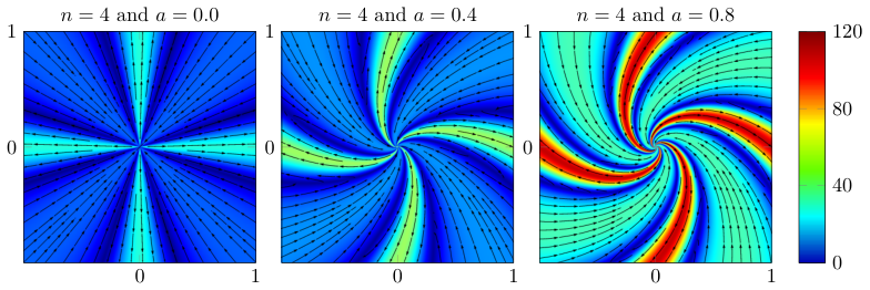
For a given $n$, the solution $\varphi$ has $n$ maxima and $n$ minima (figure 3) and the parameter $a$ has the effect of rotating the branches corresponding to these maxima or minima, as shown in figure 4. Small solutions of (1) are of particular interest because even in this case we don’t know the existence of a solution in general. Certain large solutions of the Navier-Stokes equations are known to exhibit exotic behavior at infinity, like for example the Hamel solutions which have arbitrary slow decay to infinity and violate uniqueness (Galdi, 2011, XII.2). Small solutions of the ordinary differential equation are given by $\alpha$ small, and to discuss these solutions we develop $H(\alpha)$ in a series,

$$H(\alpha)=\frac{\pi^{2}}{4}\left(1-\frac{3}{32}\alpha^{4}\right)+O(\alpha^{6})\,.$$

In view of (16), small solutions with $\Phi=0$ are only possible for $n\in\left\{1,2\right\}$. For $n=1$ and $\Phi=0$, the solutions are defined for $\left|a\right|\geq\sqrt{3}$, and we take for example $a=\sqrt{3}+\varepsilon$, with $\varepsilon>0$. We find by a series expansion, that

$$\alpha=\left(\frac{256}{3}\right)^{1/8}\varepsilon^{1/4}+O(\varepsilon^{1/2})\,,$$

and

$\displaystyle\varphi_{1}$

$\displaystyle=-4\,3^{3/4}\varepsilon^{1/2}+O(\varepsilon)\,,$

$\displaystyle\varphi_{2}$

$\displaystyle=4\,3^{3/4}\varepsilon^{1/2}+O(\varepsilon)\,,$

$\displaystyle\varphi_{3}$

$\displaystyle=6+O(\varepsilon)\,,$

and the solution satisfies

$$\varphi(z)=-4\,3^{3/4}\varepsilon^{1/2}\cos(z)+O(\varepsilon)\,.$$

Since in this case $\left|a\right|$ has to be large, we note that this does not produce a solution having a small velocity field, and the torque is also large, $M=16\pi\sqrt{3}+O(\varepsilon)$. Moreover, since $\mu+4a=0$, this corresponds to $\left|\mu\right|\geq\sqrt{48}$. This specific value is interesting since this is exactly the criterion found by Hillairet & Wittwer (2013) to obtain a solution of the Navier-Stokes equations (8b) having the asymptote $\mu\boldsymbol{e}_{\theta}/r$ for the velocity. We note that this is not in contradiction with the existence of the exact solutions found here, because the boundary condition given by the evaluation of the exact solution for $a=\sqrt{3}+\varepsilon$ is too big for the theorem of Hillairet & Wittwer (2013) to apply.

For $n=2$, we can take $a=\varepsilon$, so

$$\alpha=\left(\frac{32}{3}\right)^{1/4}\varepsilon^{1/2}+O(\varepsilon)\,,$$

and

$\displaystyle\varphi_{1}$

$\displaystyle=-4\sqrt{6}\,\varepsilon+O(\varepsilon^{2})\,,$

$\displaystyle\varphi_{2}$

$\displaystyle=4\sqrt{6}\,\varepsilon+O(\varepsilon^{2})\,,$

$\displaystyle\varphi_{3}$

$\displaystyle=6+O(\varepsilon^{2})\,,$

and the solution satisfies

$$\varphi(z)=-4\sqrt{6}\,\varepsilon\cos(2z)+O(\varepsilon^{2})\,.$$

The torque of this solution is given by $M=16\pi\varepsilon+O(\varepsilon^{2})$.

We now discuss the consequences of the existence of the newly found solutions for the solutions of the Navier-Stokes equations (9) in $\mathbb{R}^{2}$. For the reasons explained in the introduction, if $\boldsymbol{f}$ has non-zero mean, the solution can not decay like $r^{-1}$. Therefore, the new solutions describe, at best, the asymptotes of solutions for the case where $\boldsymbol{f}$ has zero mean. To discuss this question, we consider the Stokes approximation,

$$\Delta\boldsymbol{u}-\boldsymbol{\nabla}p=\boldsymbol{f}\,,$$

with $\boldsymbol{f}$ having zero mean. The asymptotic behavior of the solution to this equation is

$$\boldsymbol{u}=\frac{-1}{4\pi r}\left[\left(\cos(2\theta)\int_{\mathbb{R}^{2}}\left(x_{1}f_{1}-x_{2}f_{2}\right)+\sin(2\theta)\int_{\mathbb{R}^{2}}\left(x_{1}f_{2}+x_{2}f_{1}\right)\right)\boldsymbol{e}_{r}+\int_{\mathbb{R}^{2}}\left(\boldsymbol{x}\boldsymbol{\wedge}\boldsymbol{f}\right)\boldsymbol{e}_{\theta}\right]+O(r^{-2})\,,$$

By rotating the coordinates system, we can always make $\int_{\mathbb{R}^{2}}\left(x_{1}f_{2}+x_{2}f_{1}\right)=0$, so that the Stokes approximation has two compatibility conditions: the torque $\int_{\mathbb{R}^{2}}\left(\boldsymbol{x}\boldsymbol{\wedge}\boldsymbol{f}\right)$ and $\int_{\mathbb{R}^{2}}\left(x_{1}f_{1}-x_{2}f_{2}\right)$ which are represented in figure 2. Even if the small solution found for $n=2$ has the appropriate form $\cos(2z)$ which is similar to the $\cos(2\theta)$ of the Stokes solution, the asymptotic behavior is likely not described by this exact solution alone, because only one of the compatibility conditions can be lifted by this exact solution. In addition, we note that there are two exact solutions decaying like $r^{-1}$ and having arbitrary small torque: the harmonic function $\mu\boldsymbol{e}_{\theta}/r$ and the new solution for $n=2$. This emphasizes the wide variety of asymptotic behavior of the solutions to (9) with small data, since by truncating one of these solutions near the origin we obtain an exact solution in $\mathbb{R}^{2}$ with a certain small source term. In fact, numerical studies make us believe that even if the source term has zero mean, the solution of (9) is in general not bounded by $r^{-1}$.

References

- Galdi (2004) Galdi, G. P. 2004 Stationary Navier-Stokes problem in a two-dimensional exterior domain. In Stationary partial differential equations. Vol. I, pp. 71–155. Amsterdam: North-Holland.
- Galdi (2011) Galdi, G. P. 2011 An Introduction to the Mathematical Theory of the Navier-Stokes Equations. Steady-State Problems, 2nd edn. New York: Springer Verlag.
- Gradshteyn & Ryzhik (2007) Gradshteyn, I. & Ryzhik, I. 2007 Table of Integrals, Series, and Products, seventh edn. Academic Press.
- Guillod & Wittwer (2013) Guillod, J. & Wittwer, P. 2013 Asymptotic behaviour of solutions to the stationary Navier-Stokes equations in two dimensional exterior domains with zero velocity at infinity. arXiv:1307.6807.
- Hamel (1917) Hamel, G. 1917 Spiralförmige Bewegungen zäher Flüssigkeiten. Jahresbericht der Deutschen Mathematiker-Vereinigung 25, 34–60.
- Hillairet & Wittwer (2013) Hillairet, M. & Wittwer, P. 2013 On the existence of solutions to the planar exterior Navier Stokes system. Journal of Differential Equations 255 (10), 2996 – 3019.
- Korolev & Šverák (2011) Korolev, A. & Šverák, V. 2011 On the large-distance asymptotics of steady state solutions of the Navier-Stokes equations in 3D exterior domains. Annales de l’Institut Henri Poincaré - Analyse non linéaire 28 (2), 303–313.
- Landau (1944) Landau, L. D. 1944 A new exact solution of the Navier-Stokes equations. Doklady Akademii Nauk SSSR 43, 286–288.
- Nazarov & Pileckas (2000) Nazarov, S. A. & Pileckas, K. 2000 On steady Stokes and Navier-Stokes problems with zero velocity at infinity in a three-dimensional exterior domain. Journal of Mathematics of Kyoto University 40, 475–492.
- Nazarov & Pileckas (1999) Nazarov, S. A. & Pileckas, K. I. 1999 Asymptotic of solutions of the Navier-Stokes equations in the exterior of a bounded body. Doklady Mathematics 60 (1), 133–135.
- Rosenhead (1940) Rosenhead, L. 1940 The steady two-dimensional radial flow of viscous fluid between two inclined plane walls. Proceedings of the Royal Society of London. Series A, Mathematical and Physical Sciences 175 (963), 436–467.
- Šverák (2011) Šverák, V. 2011 On Landau’s solutions of the Navier-Stokes equations. Journal of Mathematical Sciences 179 (1), 208–228, translated from Problems in Mathematical Analysis 61, October 2011, pp. 175-190.
- Wang (1991) Wang, C. Y. 1991 Exact solutions of the steady-state Navier-Stokes equations. Annual Review of Fluid Mechanics 23, 159–177.