Exploiting Delay Correlation for Multi-Antenna-Assisted High Speed Train Communications

Delay correlation is a unique phenomenon caused by linear mobility and linearly spaced antenna array. To be specific, high speed train has deterministic moving direction and relatively steady speed in a short time. In addition, the receive array, which may utilize massive MIMO techniques, can be positioned to form a line topology in practical design. The aforementioned two assumptions form the foundation for this entire work.

Consider the toy example in Fig. 1, where two receive antennas move along the line defined by themselves. Then when Antenna 1 moves to the current position of Antenna 2 after time $\tau$, it experiences a similar channel that Antenna 2 experienced $\tau$ time ago¹¹ 1 For simplicity, assume that source S is equipped with single antenna.. In high speed scenario, $\tau$ can be so short that above mentioned two channels are almost identical. So in this case if Antenna 2 informs Antenna 1 the channel it estimated $\tau$ time ago, then Antenna 1 may save the effort for additional channel estimation. This simple but inspiring phenomenon offers even bigger advantage when the antenna number increases, as we will analyze in detail later.

Regarding correlation modeling, static scattering environment is assumed in previous works, which indicates that the channel will remain unchanged as long as the concerned antennas are immobile. However, if the ambient objects are dynamic, intuitively, there will be a decay factor attached to the cross-correlation coefficient of the diffuse counterpart. In particular, provided with the delay $\tau$ and antenna spacing $D$ for the above example, the correlation coefficient of Antenna 2 at time $t$ and Antenna 1 at time $t+\tau$ is given by the following definition.

Definition: The cross-correlation function for mobile frequency non-selective $1\times 2$ Rician fading MIMO channels is

$$\small\rho^{\textrm{DIF}}\left(\tau,D\right)=\frac{I_{0}\left(\sqrt{\kappa^{2}-\Delta^{2}-j2\kappa\Delta\cos\left(\mu-\gamma\right)}\right)}{\left(K_{R}+1\right)I_{0}\left(\kappa\right)}e^{-c_{0}v\left|\tau\right|},$$

(1)

$$\small\rho^{\textrm{LOS}}\left(\tau,D\right)=\frac{K_{R}}{K_{R}+1}e^{j\Delta\cos\left(\gamma\right)},$$

(2)

where $\Delta=2\pi\left(f_{D}\tau-\frac{D}{\lambda}\right)$ presents the location difference of the two antennas, $f_{D}=\frac{v}{\lambda}$ is the maximum Doppler shift and $\lambda$ is the signal wavelength. $\kappa$ controls the width of angle of arrival (AOA) and $\mu\in\left[-\pi,\pi\right)$ accounts for the mean direction of AOA. The mobility of the train is characterized by its velocity $v$ and direction $\gamma$. Finally, $c_{0}$ is a real-valued constant characterizing the inherent spatial property of the scattering objects.

Remarks: Some explanations for this concept are in order.

1) The cross-correlation of the diffuse part is mainly characterized by three factors: a) location difference; b) AOA difference; c) ambient objects’ movement. Apparently, static antennas and static???? scattering environment result in perfect correlation.

2) The LOS part only varies in phase of arrival, and the phase shift is obtained easily through geometric analysis.

3) This definition is in accordance with the result in [1] and may naturally be extended to multiple, even massive, antennas topology.

Based on the above definition, if $\tau$ is set as $\frac{D}{v}$, then $\Delta$ will be $0$, and finally, delay correlation is formulated. To be specific, delay correlation is characterized by

$$\small\rho^{\textrm{DIF}}\left(\tau,D\right)|_{\tau=\frac{D}{v}}=\frac{1}{K_{R}+1}e^{-c_{0}D}$$

(3)

$$\small\rho^{\textrm{LOS}}\left(\tau,D\right)|_{\tau=\frac{D}{v}}=\frac{K_{R}}{K_{R}+1}$$

(4)

Note that the direction and velocity of the train are known by both of the base station and the train.

Inspired by delay correlation, the multiple fast-fading channels between the receive antennas and and the base station is converted to a single and slow-fading channel. Therefore, repetitive channel re-estimations becomes dispensable, which will basically resolve the most challenging issue in HSTC.

Fig. 2 shows the staticized channel, which is a virtualized static channel between the source antenna and different receive antenna at different time. In particular, assume that the receiver is equipped with $N_{\textrm{R}}$ antennas. Since base station is informed of receive array spacing $D$ and velocity of the train $v$, it is reasonable to assume that base station being able to adjust the symbol time $T_{s}$ so that CSI will not change in $T_{s}$ and there exists an integer $K$ which satisfies $D=v\left(KT_{s}\right)$. By utilizing antenna selection, one antenna of the array is activated each time, marked as the dark ones in Fig. 2, to process the transmit signal. As the CSI variation of the selected antennas is negligible, channel re-estimations can be reduced in $N_{\textrm{R}}$ time slots.

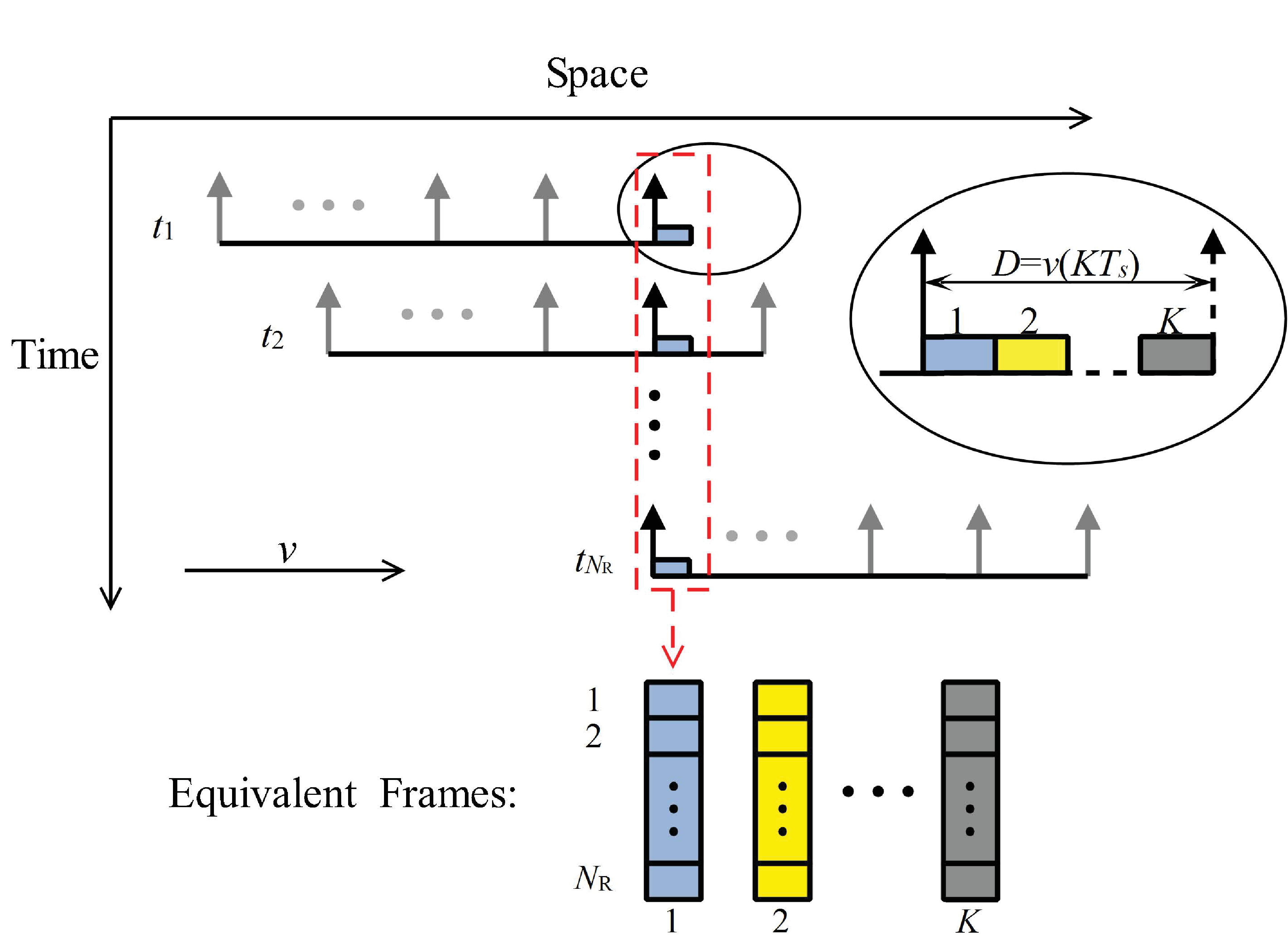
Assume Rician fading channels between S and the selected antennas $h_{i}\in\mathbb{C},i=1,\dots,N_{\textrm{R}}$. Then the signals observed at the train is given by

$$\small y_{i}=\sqrt{E_{0}}h_{i}x_{i}+n_{i},~i=1,\dots,N_{\textrm{R}}$$

(5)

where $y_{i}\in\mathbb{C}$ is the received signal, $n_{i}\in\mathbb{C}$ is the zero-mean complex Gaussian noise with covariance coefficient $\sigma^{2}_{n}$, $E_{0}$ is the average transmission energy of a symbol, scalar $x_{i}$ is the transmitted signal. To estimate the channel, several $x_{i}$ are selected to act as pilot symbols.

$\mathbf{h}=\left[h_{1}~h_{2}~\dots~h_{N_{\textrm{R}}}\right]^{T}$ is an equivalent slow fading channel. Utilizing the aforementioned delay correlation coefficients (3) and (4), the cross-correlation between $h_{p}$ and $h_{q}$, $1\leq p<q\leq N_{\textrm{R}}$, is given by

$$\small\rho^{\textrm{DIF}}_{p,q}\left(\tau,\left(q-p\right)D\right)|_{\tau=\frac{\left(q-p\right)D}{v}}=\frac{1}{K_{R}+1}e^{-c_{0}\left(q-p\right)D},$$

(6)

$$\small\rho^{\textrm{LOS}}_{p,q}\left(\tau,\left(q-p\right)D\right)|_{\tau=\frac{\left(q-p\right)D}{v}}=\frac{K_{R}}{K_{R}+1},$$

(7)

$\mathbf{x}=\left[x_{1}~x_{2}~\dots~x_{N_{\textrm{R}}}\right]^{T}$ is a vertical equivalent frame which involves $N_{\textrm{R}}$ symbols. It is noteworthy that the downlink transmission is actually divided into many successive staticized blocks, each lasts for a period of $N_{\textrm{R}}\times KT_{s}$, so there will be $K$ frames received in a block as depicted in Fig.2.

With $\mathbf{h}$ and $\mathbf{x}$ defined above, we formalize the system model as

$$\small\mathbf{y}=\sqrt{E_{0}}\mathbf{X}\mathbf{h}+\mathbf{n},$$

(8)

where $\mathbf{y}=\left[y_{1}~y_{2}~\dots~y_{N_{\textrm{R}}}\right]^{T}\in\mathbb{C}^{N_{\textrm{R}}\times 1}$ is the received vertical vector, $\mathbf{n}=\left[n_{1}~n_{2}~\dots~n_{N_{\textrm{R}}}\right]^{T}\in\mathbb{C}^{N_{\textrm{R}}\times 1}$ is the vertical noise vector with covariance matrix $\mathbf{R}_{n}=\sigma^{2}_{n}\mathbf{I}_{N_{\textrm{R}}}$, $\mathbf{X}$ is a size-$N_{\textrm{R}}$ diagonal matrix with $\mathbf{x}$ on its diagonal.

The Two-Step MMSE scheme proposed in [17] is employed for channel estimation. It decomposes the channel estimation into two steps, i.e., channel estimation at pilot locations and channel interpolation. With similar definitions, $N_{\textrm{R}}$ time slots are divided into $N_{s}$ data symbols and $N_{p}\leq N_{s}$ pilot symbols. $N_{\textrm{R}}$, $N_{s}$ and $N_{p}$ can be chosen such that $L=\frac{N_{s}}{N_{p}}$ is an integer. The pilot symbols are equally spaced such that two adjacent pilot symbols are interpolated by $L$ data symbols. In this sense, the pilot percentage is $\delta=\frac{1}{L+1}$. Assume that the stationary LOS part of Rician fading channel $h^{\textrm{LOS}}$ is perfectly estimated, which implies that channel estimation will only apply to the diffuse component $h^{\textrm{DIF}}$. Hence, using the model in (5), the mean square error (MSE) of the $i-$th channel coefficient is

$$\small\sigma_{i}^{2}=\textrm{E}\left[\left|\hat{h}_{i}-h_{i}\right|^{2}\right]=\textrm{E}\left[\left|\hat{h}_{i}^{\textrm{DIF}}-h_{i}^{\textrm{DIF}}\right|^{2}\right],~i=1,\dots,N_{\textrm{R}},$$

(9)

where $\hat{h}_{i}$ is an estimation of $h_{i}$.

Firstly, the receiver obtains the channel estimations at pilot locations. Assume that $\mathbf{P}$, $\mathbf{h}_{p}$ and $\mathbf{y}_{p}$ are the pilot symbols and their corresponding fading channels, received symbols extracted from $\mathbf{X}$, $\mathbf{h}$ and $\mathbf{y}$, respectively. Then the received pilot symbols are expressed as

$$\small\mathbf{y}_{p}=\sqrt{E_{0}}\mathbf{P}\mathbf{h}_{p}+\mathbf{n}_{p},$$

(10)

The receive array derives the channel estimations by minimizing the average MSE, $\sigma_{\textrm{avg}}^{2}=\frac{1}{N_{p}}\textrm{E}[\|\hat{\mathbf{h}}_{p}^{\textrm{DIF}}-\mathbf{h}_{p}^{\textrm{DIF}}\|^{2}]$. Its solution is

$$\small\hat{\mathbf{h}}_{p}^{\textrm{DIF}}=\mathbf{W}_{p}^{H}\left(\mathbf{y}_{p}-\sqrt{E_{0}}\mathbf{P}\mathbf{h}_{p}^{\textrm{LOS}}\right),$$

(11)

where $\hat{\mathbf{h}}_{p}^{\textrm{DIF}}\in\mathbb{C}^{N_{p}\times 1}$ is the estimation of $\mathbf{h}_{p}^{\textrm{DIF}}$, and $\mathbf{W}_{p}=\sqrt{E_{0}}(E_{0}\mathbf{P}\mathbf{R}_{hh}^{\textrm{DIF}}\mathbf{P}^{H}+\sigma^{2}_{n}\mathbf{I}_{N_{p}})^{-1}\mathbf{P}\mathbf{R}_{hh}^{\textrm{DIF}}$ is the channel MMSE estimation matrix, auto-correlation matrix of the diffuse channel $\mathbf{R}_{hh}^{\textrm{DIF}}=\textrm{E}\left[\mathbf{h}_{p}^{\textrm{DIF}}\left(\mathbf{h}_{p}^{\textrm{DIF}}\right)^{H}\right]\in\mathbb{R}^{N_{p}\times N_{p}}$ is a Toeplitz matrix whose $\left(m,n\right)$-th element being

$$\small\rho_{m,n}=\rho_{m,n}^{\textrm{DIF}}=\frac{1}{K_{R}+1}e^{-c_{0}\left|m-n\right|\frac{D}{\delta}},$$

(12)

where $\delta$ is the pilot percentage.

In the second step, the channel estimation of arbitrary $h_{i}$ is obtained through interpolating $\hat{\mathbf{h}}_{p}^{\textrm{DIF}}$ and attaching the LOS component

$$\small\hat{h}_{i}=\mathbf{w}_{d}^{H}\hat{\mathbf{h}}_{p}^{\textrm{DIF}}+h_{i}^{\textrm{LOS}},$$

(13)

where the real-valued coefficient vector $\mathbf{w}_{d}\in\mathbb{R}^{N_{p}\times 1}$ is designed according to the MSE minimization criterion (9).

It is proved in [17] that this scheme is equivalent to the optimum linear MMSE estimator as follows

$$\small\begin{split}\hat{h}_{i}=&\sqrt{E_{0}}\mathbf{r}_{i}^{\textrm{DIF}}\mathbf{P}^{H}(E_{0}\mathbf{P}\mathbf{R}_{hh}^{\textrm{DIF}}\mathbf{P}^{H}+\sigma^{2}_{n}\mathbf{I}_{N_{p}})^{-1}\times\\ &\left(\mathbf{y}_{p}-\sqrt{E_{0}}\mathbf{P}\mathbf{h}_{p}^{\textrm{LOS}}\right)+h_{i}^{\textrm{LOS}},~i=1,\dots,N_{\textrm{R}},\end{split}$$

(14)

where $\mathbf{r}_{i}^{\textrm{DIF}}=\textrm{E}\left[h_{i}^{\textrm{DIF}}\left(\mathbf{h}_{p}^{\textrm{DIF}}\right)^{H}\right]$, which indicates that $\mathbf{w}_{d}^{H}=\mathbf{r}_{i}^{\textrm{DIF}}\left(\mathbf{R}_{hh}^{\textrm{DIF}}\right)^{-1}$.

The accuracy of channel estimation is mainly determined by pilot percentage. Meanwhile, imperfect channel estimation results in high error probability[18]. Hence, there exists a mapping between error probability $P_{e}$ and pilot percentage $\delta$.

Above all, the MSE of the Two-Step MMSE estimation scheme is derived. As stated in [6], define the error correlation matrix at pilot locations as

$$\small\mathbf{R}_{ee}=\textrm{E}\left[\mathbf{e}_{p}\mathbf{e}_{p}^{H}\right],$$

(15)

where $\mathbf{e}_{p}=\hat{\mathbf{h}}_{p}-\mathbf{h}_{p}=\hat{\mathbf{h}}_{p}^{\textrm{DIF}}-\mathbf{h}_{p}^{\textrm{DIF}}$. For simplicity, assume that the pilot symbols $\mathbf{P}=\mathbf{I}_{N_{p}}$. Substituting this assumption and (10)(11) into (15), it can be calculated that

$$\small\mathbf{R}_{ee}=\mathbf{R}_{hh}^{\textrm{DIF}}-\mathbf{R}_{hh}^{\textrm{DIF}}\left(\mathbf{R}_{hh}^{\textrm{DIF}}+\frac{1}{\gamma}\mathbf{I}_{N_{p}}\right)^{-1}\mathbf{R}_{hh}^{\textrm{DIF}},$$

(16)

where $\gamma=\frac{E_{0}}{\sigma_{n}^{2}}$ is the signal-to-noise ratio (SNR). Then the average MSE at pilot locations is

$$\small\sigma_{p,N_{p}}^{2}=\frac{1}{N_{p}}\textrm{trace}\left(\mathbf{R}_{ee}\right),$$

(17)

Through asymptotic analysis, i.e., $N_{p}\rightarrow\infty$, $N_{s}\rightarrow\infty$ and $N_{\textrm{R}}\rightarrow\infty$, with a finite pilot percentage $\delta$, the asymptotic MSE at pilot locations can be expressed as a function of $\delta$ with the following theorem. Note that asymptotic analysis is reasonable for massive MIMO where a large amount of receiver antennas exist.

Intuitively, more pilot symbols result in better channel estimations, which would help improve the spectral efficiency. On the other hand, excessive pilot symbols would lead to unnecessary spectrum overhead. Hence, there exists an optimal pilot percentage which would maximize the spectral efficiency. [6] gives the maximum spectral efficiency analysis with imperfect channel information in Rayleigh fading channels. In a similar fashion, the relation between spectral efficiency $\eta$ and pilot percentage $\delta$ in Rician fading models will be obtained.

In this paper, the effective spectral efficiency is defined as

$$\small\eta=\frac{N_{s}}{N_{\textrm{R}}}\textrm{E}_{\hat{h}}\left[C\left(\hat{h},\gamma\right)\right]=\left(1-\delta\right)\textrm{E}_{\hat{h}}\left[C\left(\hat{h},\gamma\right)\right],$$

(30)

where $C(\hat{h},\gamma)$ is the channel capacity with imperfect channel estimations $\hat{h}$ and SNR $\gamma$.

After SNR $\gamma$ and pilot percentage $\delta$ are specified, the corresponding MSE at data symbol locations can be calculated through (24). Furthermore, the average error probability $P_{e}$ and spectral efficiency $\eta_{up}$ can be derived through (29) and (35), respectively. Evidently, it is unrealistic to simultaneously achieve lower $P_{e}$ and higher $\eta_{up}$, thus implying a tradeoff relation between them.

According to (32), it is possible to obtain the maximum spectral efficiency through selecting a specific $\delta_{\textrm{SE-opt}}$, yet the corresponding BER performance would not necessarily be satisfactory. However, it is worth nothing that $\delta_{\textrm{SE-opt}}$ has practical implication in our tradeoff analysis, i.e., it would serve as the lower bound of feasible pilot percentages. When $\delta>\delta_{\textrm{SE-opt}}$, both spectral efficiency and error probability would decrease monotonically. Hence, it is crucial to choose a pilot percentage between $\delta_{\textrm{SE-opt}}$ and $0.5$ to balance between error probability and spectral efficiency.

Having understood the relation among MSE, error probability and spectral efficiency, it makes sense to adjust $\delta$ between $\delta_{\textrm{SE-opt}}$ and $0.5$ while calculating the corresponding $P_{e}$ and $\eta_{up}$, thus obtaining the optimal tradeoff between error probability and spectral efficiency.

(17) is equal to summarizing the eigenvalues of $\frac{1}{N_{p}}\mathbf{R}_{ee}$ as follows

$$\small\begin{split}\sigma_{p,N_{p}}^{2}&=\frac{1}{N_{p}}\sum_{n=1}^{N_{p}}\left[\lambda_{n}-\left(\lambda_{n}+\frac{1}{\gamma}\right)^{-1}\lambda_{n}^{2}\right]\\ &=\frac{1}{N_{p}}\sum_{n=1}^{N_{p}}\left(\frac{\lambda_{n}}{\lambda_{n}\gamma+1}\right)\end{split}$$

(36)

where $\lambda_{n}$ is the $n$-th eigenvalue of $\mathbf{R}_{hh}$. Based on the asymptotic analysis method in [20], when $N_{p}\rightarrow\infty$, $\sigma_{p,N_{p}}^{2}$ can be recast as

$$\small\sigma_{p}^{2}=\lim_{N_{p}\rightarrow\infty}\sigma_{p,N_{p}}^{2}=\frac{1}{2\pi}\int_{-\pi}^{\pi}\left[\frac{\Lambda\left(\Omega\right)}{\Lambda\left(\Omega\right)\gamma+1}\right]d\Omega$$

(37)

where $\Lambda\left(\Omega\right)$ is the discrete-time Fourier transform (DTFT) of $\left\{\frac{1}{K_{R}+1}e^{-c_{0}\left|k\right|\frac{D}{\delta}}\right\}_{k}$, which is expressed as

$$\small\begin{split}\Lambda\left(\Omega\right)&=\sum_{k=-\infty}^{\infty}\left(\frac{1}{K_{R}+1}e^{-c_{0}\left|k\right|\frac{D}{\delta}}\right)e^{-jk\Omega}\\ &=\frac{1}{K_{R}+1}\left[\frac{1-\alpha^{2}}{1-2\alpha\textrm{cos}(\Omega)+\alpha^{2}}\right]\end{split}$$

(38)

where $\alpha=e^{-c_{0}\frac{D}{\delta}}$. Therefore, $\sigma_{p}^{2}$ could be calculated by

$$\small\begin{split}\sigma_{p}^{2}&=\frac{1}{2\pi}\int_{-\pi}^{\pi}\left[\frac{\frac{1}{K_{R}+1}}{\frac{\gamma}{K_{R}+1}+\frac{1+\alpha^{2}}{1-\alpha^{2}}-\frac{2\alpha}{1-\alpha^{2}}\textrm{cos}\left(\Omega\right)}\right]d\Omega\\ &=\frac{1}{K_{R}+1}\times\sqrt{\frac{1}{a^{2}-b^{2}}}\end{split}$$

(39)

where $a=\frac{\gamma}{K_{R}+1}+\frac{1+\alpha^{2}}{1-\alpha^{2}}$ and $b=-\frac{2\alpha}{1-\alpha^{2}}$.

The same with (36) and (37), $\sigma_{d,u,N_{p}}^{2}$ can be rewritten as

$$\small\sigma_{d,u}^{2}=\frac{1}{2\pi}\int_{-\pi}^{\pi}\left[\Lambda\left(\Omega\right)-\frac{\left|\Lambda_{dh,u}\left(\Omega\right)\right|^{2}}{\Lambda\left(\Omega\right)+\frac{1}{\gamma}}\right]d\Omega$$

(40)

$\Lambda_{dh,u}\left(\Omega\right)$ is the DTFT of $\left\{\frac{1}{K_{R}+1}e^{-c_{0}\left|k+\delta u\right|\frac{D}{\delta}}\right\}_{k}$ and is expressed as

$$\small\Lambda_{dh,u}\left(\Omega\right)=\frac{1}{K_{R}+1}\left[\frac{\alpha\left(\beta^{-1}-\beta\right)e^{j\Omega}+\beta-\alpha^{2}\beta^{-1}}{1-2\alpha\textrm{cos}(\Omega)+\alpha^{2}}\right]$$

(41)

where $\beta=e^{-c_{0}uD}$. Substituting (38) and (41) into (40), $\sigma_{d,u}^{2}$ could be recast as the form in (24).

The capacity $C(\hat{h},\gamma)$ is equivalent to the maximum conditional mutual information $\max\{\textrm{I}(x;y|\hat{h})\}$, where $\textrm{I}(x;y|\hat{h})$ is defined below

$$\small\textrm{I}\left(x;y|\hat{h}\right)=\textrm{E}_{x,y}\left[\log p\left(y|x,\hat{h}\right)\right]-\textrm{E}_{y}\left[\log p\left(y|\hat{h}\right)\right]$$

(42)

where $x$ is a symbol of the $u$-th group, $\hat{h}$ and $y$ are the corresponding estimated channel coefficient and received signal. Conditional on $\hat{h}$ and $x$, $y$ is Gaussian distributed with mean and variance given in [6]

$$\small\mu_{y|x,\hat{h}}=\sqrt{E_{0}}\hat{h}x$$

(43)

$$\small\sigma_{y|x,\hat{h}}^{2}=E_{0}\sigma_{d,u}^{2}+\sigma_{n}^{2}$$

(44)

$\left|x_{u}\right|=1$ is utilized in the second equation. Therefore,

$$\small\textrm{E}_{x,y}\left[\log p\left(y|x,\hat{h}\right)\right]=\log\frac{1}{\pi e\left(E_{0}\sigma_{d,u}^{2}+\sigma_{n}^{2}\right)}$$

(45)

Note that $h-\hat{h}\sim\textrm{CN}(0,\sigma_{d,u}^{2})$, so the mean and variance of $y$ conditional on $\hat{h}$ are

$$\small\mu_{y|\hat{h}}=0$$

(46)

$$\small\sigma_{y|\hat{h}}^{2}=E_{0}\left(|\hat{h}|^{2}+\sigma_{d,u}^{2}\right)+\sigma_{n}^{2}$$

(47)

$\textrm{I}(x;y|\hat{h})$ is maximized when $y|\hat{h}$ is Gaussian distributed. However, $y|\hat{h}$ is not Gaussian distributed in practise. In this case,

$$\small-\textrm{E}_{y}\left[\log p\left(y|\hat{h}\right)\right]\leq\log\left(\pi e\left(E_{0}\left(|\hat{h}|^{2}+\sigma_{d,u}^{2}\right)+\sigma_{n}^{2}\right)\right)$$

(48)

Substituting (45) and (48) into (42) completes the proof.

Since $h$ is Rician distributed with parameters $\nu=\sqrt{\frac{K_{R}}{K_{R}+1}}$ and $\sigma=\sqrt{\frac{1}{2(K_{R}+1)}}$, i.e., $h\sim\textrm{Rice}\left(\sqrt{\frac{K_{R}}{K_{R}+1}},\sqrt{\frac{1}{2(K_{R}+1)}}\right)$. Hence, $|\sqrt{2(K_{R}+1)}h|^{2}$ accords with a noncentral chi-squared distribution with two degrees of freedom and noncentrality parameter $2K_{R}$.

Combining (11), (20) and (22), it could be obtained that

$$\small\mathbf{R}_{\hat{d}\hat{d},u}=\frac{K_{R}}{K_{R}+1}\mathbf{I}_{N_{p}}+\mathbf{R}_{\hat{d}\hat{d},u}^{\textrm{DIF}}=\mathbf{I}_{N_{p}}-\mathbf{\Psi}_{ee,u}$$

(49)

From (49), $\textrm{E}[|\hat{h}|^{2}]$ is given by

$$\small\textrm{E}[|\hat{h}|^{2}]=\lim_{N_{p}\rightarrow\infty}\frac{1}{N_{p}}\mathbf{R}_{\hat{d}\hat{d},u}=1-\sigma^{2}_{d,u}$$

(50)

$|h|^{2}$ and $|\hat{h}|^{2}$ are of highly correlated distributions. Moreover, (50) implies that $\textrm{E}[|\hat{h}|^{2}]\approx\textrm{E}[|h|^{2}]$. As a consequence, it is practical to use $|h|^{2}$ to approximate $|\hat{h}|^{2}$. Therefore,

$$\small C(\hat{h},\gamma)_{u}\approx\log\left(1+\frac{|\sqrt{2(K_{R}+1)}h|^{2}}{2\left(K_{R}+1\right)\left(\sigma_{d,u}^{2}+\frac{1}{\gamma}\right)}\right)$$

(51)

and

$$\small\eta\approx\left(1-\delta\right)\int_{0}^{+\infty}\log\left(1+\frac{x}{2\left(K_{R}+1\right)\left(\sigma_{d,u}^{2}+\frac{1}{\gamma}\right)}\right)p\left(x\right)dx$$

(52)

where $p\left(x\right)$ is the probability density function of $|\sqrt{2(K_{R}+1)}h|^{2}$, which could be expressed as

$$\small p\left(x\right)=\frac{1}{2}e^{-\frac{x+2K_{R}}{2}}I_{0}\left(\sqrt{2K_{R}x}\right)$$

(53)

$I_{n}(z)$ is $n$-th order modified Bessel function of the first kind.

References

- [1] A. Abdi and M. Kaveh, “A space-time correlation model for multielement antenna systems in mobile fading channels,” Selected Areas in Communications, IEEE Journal on, vol. 20, no. 3, pp. 550–560, 2002.
- [2] IST-WINNER, “Deliverable 1.1.2 v.1.2, WINNER II Channel Models,” Tech. Rep., 2008 (http://projects.celtic-initiative.org/winner+/deliverables. html), Tech. Rep., 2007.
- [3] X. Ma, G. B. Giannakis, and S. Ohno, “Optimal training for block transmissions over doubly selective wireless fading channels,” Signal Processing, IEEE Transactions on, vol. 51, no. 5, pp. 1351–1366, 2003.
- [4] R. Negi and J. Cioffi, “Pilot tone selection for channel estimation in a mobile OFDM system,” Consumer Electronics, IEEE Transactions on, vol. 44, no. 3, pp. 1122–1128, 1998.
- [5] I. Barhumi, G. Leus, and M. Moonen, “Optimal training design for MIMO OFDM systems in mobile wireless channels,” Signal Processing, IEEE Transactions on, vol. 51, no. 6, pp. 1615–1624, 2003.
- [6] N. Sun and J. Wu, “Maximizing spectral efficiency for high mobility systems with imperfect channel state information,” Wireless Communications, IEEE Transactions on, 2014, accepted (to be published).
- [7] M. Grossglauser and D. Tse, “Mobility increases the capacity of ad-hoc wireless networks,” in INFOCOM 2001. Twentieth Annual Joint Conference of the IEEE Computer and Communications Societies. Proceedings. IEEE, vol. 3. IEEE, 2001, pp. 1360–1369.
- [8] L. Sun and W. Wang, “On latency distribution and scaling: from finite to large cognitive radio networks under general mobility,” in INFOCOM, 2012 Proceedings IEEE. IEEE, 2012, pp. 1287–1295.
- [9] X. Lu, J. L. Tiffany, Y. Liu, and C. Yuen, “A novel siso trellis strategy for relaying distorted signals in wireless networks,” in Communications (ICC), 2013 IEEE International Conference on. IEEE, 2013, pp. 5247–5251.
- [10] H. Zhang, Z. Zhang, and H. Dai, “Gossip-based information spreading in mobile networks,” Wireless Communications, IEEE Transactions on, vol. 12, no. 11, pp. 5918–5928, 2013.
- [11] L. Sun and W. Wang, “On distribution and limits of information dissemination latency and speed in mobile cognitive radio networks,” in INFOCOM, 2011 Proceedings IEEE. IEEE, 2011, pp. 246–250.
- [12] X. Chen and C. Yuen, “Efficient resource allocation in a rateless-coded mu-mimo cognitive radio network with qos provisioning and limited feedback,” Vehicular Technology, IEEE Transactions on, vol. 62, no. 1, pp. 395–399, 2013.
- [13] X. Chen and H. Chen, “Interference-aware resource control in multi-antenna cognitive ad hoc networks with heterogeneous delay constraints,” IEEE Communication Letter, vol. 17, no. 6, pp. 1184–1187, 2013.
- [14] D. Gesbert, M. Shafi, D.-s. Shiu, P. J. Smith, and A. Naguib, “From theory to practice: an overview of MIMO space-time coded wireless systems,” Selected Areas in Communications, IEEE Journal on, vol. 21, no. 3, pp. 281–302, 2003.
- [15] A. F. Molisch, “A generic model for MIMO wireless propagation channels in macro-and microcells,” Signal Processing, IEEE Transactions on, vol. 52, no. 1, pp. 61–71, 2004.
- [16] K. I. Pedersen, J. B. Andersen, J. P. Kermoal, and P. Mogensen, “A stochastic multiple-input-multiple-output radio channel model for evaluation of space-time coding algorithms,” in Vehicular Technology Conference, 2000. IEEE-VTS Fall VTC 2000. 52nd, vol. 2. IEEE, 2000, pp. 893–897.
- [17] J. Wu and N. Sun, “Optimum sensor density in distortion-tolerant wireless sensor networks,” Wireless Communications, IEEE Transactions on, vol. 11, no. 6, pp. 2056–2064, 2012.
- [18] W. M. Gifford, M. Z. Win, and M. Chiani, “Diversity with practical channel estimation,” Wireless Communications, IEEE Transactions on, vol. 4, no. 4, pp. 1935–1947, 2005.
- [19] J. Wu and C. Xiao, “Optimal diversity combining based on linear estimation of Rician fading channels,” Communications, IEEE Transactions on, vol. 56, no. 10, pp. 1612–1615, 2008.
- [20] H. Gazzah, P. A. Regalia, and J.-P. Delmas, “Asymptotic eigenvalue distribution of block toeplitz matrices and application to blind simo channel identification,” Information Theory, IEEE Transactions on, vol. 47, no. 3, pp. 1243–1251, 2001.