User Cooperation in Wireless Powered Communication Networks

Energy harvesting has recently received a great deal of attention in wireless communication since it provides virtually perpetual energy supplies to wireless networks through scavenging energy from the environment. In particular, harvesting energy from the far-field radio-frequency (RF) signal transmissions is a promising solution, which opens a new avenue for the unified study of wireless energy transfer (WET) and wireless information transmission (WIT) as radio signals are able to carry energy and information at the same time.

There are two main paradigms of research along this direction. One line of work aims to characterize the fundamental trade-offs in simultaneous WET and WIT with the same transmitted signal in the so-called simultaneous wireless information and power transfer (SWIPT) systems (see e.g., [1]-[3] and the references therein). Another line of research focuses on designing a new type of wireless network termed wireless powered communication network (WPCN) in which wireless terminals communicate using the energy harvested from WET (see e.g., [4]-[6]).

In our previous work [6], we studied a typical WPCN model, in which one hybrid access-point (H-AP) coordinates WET/WIT to/from a set of distributed users in the downlink (DL) and uplink (UL) transmissions, respectively. It has been shown in [6] that the WPCN suffers from a so-called “doubly near-far” problem, which occurs when a far user from the H-AP receives less wireless energy than a near user in the DL, but needs to transmit with more power in the UL for achieving the same communication performance due to the doubled distance-dependent signal attenuation over both the DL and UL. As a result, unfair rate allocations among the near and far users are inured when their sum-throughput is maximized. In [6], we proposed to assign shorter/longer time to the near/far users in their UL WIT to solve the doubly near-far problem, which is shown to achieve more fair rate allocations among the users in a WPCN.

On the other hand, user cooperation is an effective way to improve the capacity, coverage, and/or diversity performance in conventional wireless communication systems. Assuming constant energy supplies at user terminals, cooperative communication has been thoroughly investigated in the literature under various protocols such as decode-and-forward and amplify-and-forward (see e.g., [7], [8] and the references therein). Recently, cooperative communication has been studied in energy harvesting wireless communication and SWIPT systems (see e.g. [9]-[11]). However, how to exploit user cooperation in the WPCN to overcome the doubly near-far problem and further improve the network throughput and user fairness still remains unknown, which motivates this work.

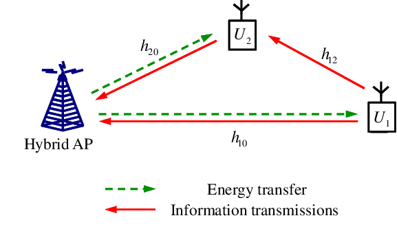
In this paper, we study user cooperation in the WPCN for throughput optimization. For the purpose of exposition, we consider a two-user WPCN, as shown in Fig. 1, where one H-AP broadcasts wireless energy to two distributed users with different distances in the DL, and the two users transmit their independent information using individually harvested energy to the H-AP in the UL through time-division-multiple-access (TDMA). To enable user cooperation, we propose that the near user which has a better channel than the far user for both DL WET and UL WIT uses part of its allocated UL time and DL harvested energy to first help to relay the information of the far user to the H-AP and then uses the remaining time and energy to transmit its own information. Under this protocol, we characterize the maximum weighted sum-rate (WSR) of the two users by jointly optimizing the time and power allocations in the network for both WET in the DL and WIT in the UL, subject to a given total time constraint. The achievable throughput gain in the WPCN by the proposed user cooperation scheme is shown both analytically and through simulations over the baseline scheme in [6] without user cooperation.

The rest of this paper is organized as follows. Section II presents the system model of the WPCN with user cooperation. Section III presents the time and power allocation problem to maximize the WSR in the WPCN, and compares the solutions and achievable throughput regions with versus without user cooperation. Section IV presents more simulation results under practical fading channel setups. Finally, Section V concludes the paper.

As shown in Fig. 1, this paper considers a two-user WPCN with WET in the DL and WIT in the UL. The network consists of one hybrid access point (H-AP) and two users (e.g., sensors) denoted by $U_{1}$ and $U_{2}$, respectively, operating over the same frequency band. The H-AP and the users are assumed to be each equipped with one antenna. Furthermore, it is assumed that the H-AP has a constant energy supply (e.g., battery), whereas $U_{1}$ and $U_{2}$ need to replenish energy from the received signals broadcast by the H-AP in the DL, which is then stored and used to maintain their operations (e.g., sensing and data processing) and also communicate with the H-AP in the UL.

We assume without loss of generality that $U_{2}$ is nearer to the H-AP than $U_{1}$, and hence denote the distance between the H-AP and $U_{1}$, that between the H-AP and $U_{2}$, and that between the $U_{1}$ and $U_{2}$ as $D_{10}$, $D_{20}$, and $D_{12}$, respectively, with $D_{10}\geq D_{20}$. We also assume that $D_{12}\leq D_{10}$ so that $U_{2}$ can more conveniently decode the information sent by $U_{1}$ than the H-AP, to motivate the proposed user cooperation to be introduced next. Assuming that the channel reciprocity holds between the DL and UL, then the DL channel from the H-AP to user $U_{i}$ and the corresponding reversed UL channel are both denoted by a complex random variable $\tilde{h}_{i0}$ with channel power gain $h_{i0}={|\tilde{h}_{i0}|^{2}}$, $i=1,2$, which in general should take into account the distance-dependent signal attenuation and long-term shadowing as well as the short-term fading. In addition, the channel from $U_{1}$ to $U_{2}$ is denoted by a complex random variable $\tilde{h}_{12}$ with channel power gain $h_{12}={|\tilde{h}_{12}|^{2}}$. If only the distance-dependent signal attenuation is considered, we should have $h_{10}\leq h_{12}$ and $h_{10}\leq h_{20}$ due to the assumptions of $D_{10}\geq D_{20}$ and $D_{10}\geq D_{12}$. Furthermore, we consider block-based transmissions over quasi-static flat-fading channels, where $h_{10}$, $h_{20}$, and $h_{12}$ are assumed to remain constant during each block transmission time, denoted by $T$, but can vary from one block to another. In each block, it is further assumed that the H-AP has the perfect knowledge of $h_{10}$, $h_{20}$, and $h_{12}$, and $U_{2}$ knows perfectly $h_{12}$.

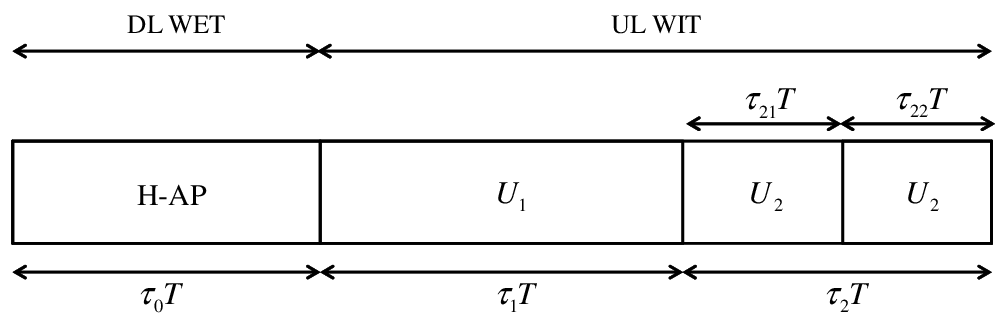
We extend the harvest-then-transmit protocol proposed in [6] for the two-user WPCN to enable user cooperation, as shown in Fig. 2. In each block, during the first $\tau_{0}T$ amount of time, $0<\tau_{0}<1$, the H-AP broadcasts wireless energy to both $U_{1}$ and $U_{2}$ in the DL with fixed transmit power $P_{0}$. The far user $U_{1}$ then transmits its information with average power $P_{1}$ during the subsequent $\tau_{1}T$ amount of time in the UL, $0<\tau_{1}<1$, using its harvested energy, and both the H-AP and $U_{2}$ decode the received signal from $U_{1}$. To overcome the doubly near-far problem [6], during the remaining $(1-\tau_{0}-\tau_{1})T$ amount of time in each block, the near user $U_{2}$ first relays the far user $U_{1}$’s information and then transmits its own information to the H-AP using its harvested energy with average power $P_{21}$ over $\tau_{21}T$ amount of time and with average power $P_{22}$ over $\tau_{22}T$ amount of time, respectively, where $\tau_{21}+\tau_{22}=\tau_{2}$. Note that we have a total time constraint given by

$${\sum\limits_{i=0}^{2}{{\tau_{i}}}=\tau_{0}+\tau_{1}+\tau_{21}+\tau_{22}\leq 1.}$$

(1)

For convenience, we noramlize $T=1$ in the sequel without loss of generality.

During the DL phase, the transmitted complex baseband signal of the H-AP in one block of interest is denoted by an arbitrary random signal, $x_{0}$, satisfying $\mathbb{E}[{{{\left|{{x_{0}}}\right|}^{2}}}]=P_{0}$. The received signal at $U_{i}$, $i=1,2$, is then expressed as

$${{y_{i}^{(0)}}=\sqrt{h_{i\,0}}{x_{0}}+{z_{i}},\,\,\,\,\,\,i=1,2,}$$

(2)

where $y_{r}^{(k)}$ denotes the received signal at $U_{r}$ during $\tau_{k}$, with $k\in\left\{{0,1,21,22}\right\}$ and $r\in\left\{{0,1,2}\right\}$ (with $U_{0}$ denoting the H-AP in the sequel). In (2), ${z_{i}}$ denotes the received noise at $U_{i}$ which is assumed to be ${z_{i}}\sim{\mathcal{CN}}\left({0,\sigma_{i}^{2}}\right)$, $i=1,2$, where ${\mathcal{CN}}({\mu,\sigma^{2}})$ stands for a circularly symmetric complex Gaussian (CSCG) random variable with mean $\mu$ and variance $\sigma^{2}$. It is assumed that $P_{0}$ is sufficiently large such that the energy harvested due to the receiver noise is negligible and thus is ignored. Hence, the amount of energy harvested by each user in the DL can be expressed as (assuming unit block time, i.e., $T=1$)

$${{E_{i}}={\zeta_{i}}{P_{0}}{h_{i0}}{\tau_{0}},\,\,\,\,\,\,i=1,2,}$$

(3)

where $0<\zeta_{i}<1$, $i=1,2$, is the energy conversion efficiency at the receiver of $U_{i}$.

After the DL phase, each user uses a fixed portion of its harvested energy, denoted by $\eta_{i}$, with $0<\eta_{i}\leq 1$, $i=1,2$, for the UL transmissions, i.e., transmitting own information (by both $U_{1}$ and $U_{2}$) or relaying the other user’s information (by $U_{2}$ only) to the H-AP. Within the first $\tau_{1}$ amount of time allocated to $U_{1}$, the average transmit power of $U_{1}$ is given by

$${{P_{1}}=\frac{{{\eta_{1}}{E_{1}}}}{{{\tau_{1}}}}={\eta_{1}}{\zeta_{1}}{P_{0}}{h_{10}}\frac{{{\tau_{0}}}}{{{\tau_{1}}}}.}$$

(4)

We denote $x_{1}$ as the complex baseband signal transmitted by $U_{1}$ with power $P_{1}$, which is assumed to be Gaussian, i.e., ${x_{1}}\sim{\mathcal{CN}}\left({0,P_{1}}\right)$. The received signals at the H-AP and $U_{2}$ in this UL slot for $U_{1}$ are expressed, respectively, as

$${y_{i}^{(1)}=\sqrt{{h_{1i}}}\,{x_{1}}+{z_{i}},\,\,i=0,\,2,}$$

(5)

where ${z_{0}}\sim{\mathcal{CN}}\left({0,\sigma_{0}^{2}}\right)$ denotes the receiver noise at the H-AP.

During the last $\tau_{2}$ amount of time allocated to $U_{2}$, the total energy consumed by $U_{2}$ for transmitting its own information and relaying the decoded information for $U_{1}$ should be no larger than $\eta_{2}E_{2}$, i.e.,

$${\tau_{21}P_{21}+\tau_{22}P_{22}\leq\eta_{2}{\zeta_{2}}{P_{0}}{h_{20}}{\tau_{0}}.}$$

(6)

We denote the complex basedband signals transmitted by $U_{2}$ for relaying $U_{1}$’s information and transmitting its own information as $x_{21}$ with power $P_{21}$ and $x_{22}$ with power $P_{22}$, respectively, where ${x_{21}}\sim{\mathcal{CN}}\left({0,P_{21}}\right)$ and ${x_{22}}\sim{\mathcal{CN}}\left({0,P_{22}}\right)$. During $\tau_{21}$ and $\tau_{22}$ amount of time allocated to $U_{2}$, the corresponding received signals at the H-AP can be expressed as

$${y_{0}^{(2i)}=\sqrt{{h_{20}}}\,{x_{2i}}+{z_{0}},\,\,i=1,\,2.}$$

(7)

Denote the time allocations to DL WET and UL WIT as $\boldsymbol{\tau}=[\tau_{0},\,\,\tau_{1},\,\,\tau_{21},\,\,\tau_{22}]$, and the transmit power values of $U_{1}$ and $U_{2}$ for UL WIT as ${\bf{P}}=[P_{1},\,\,P_{21},\,\,P_{22}]$. From [8], the achievable rate of $U_{1}$ for a given pair of $\boldsymbol{\tau}$ and ${\bf{P}}$ can be expressed from (5) and (7) as

$${R_{1}\left({\boldsymbol{\tau},{\bf{P}}}\right)=\min\left[{{R_{1}^{(10)}}\left({\boldsymbol{\tau},{\bf{P}}}\right)+{R_{1}^{(20)}}\left({\boldsymbol{\tau},{\bf{P}}}\right),\,\,{R_{1}^{(12)}}\left({\boldsymbol{\tau},{\bf{P}}}\right)}\right],}$$

(8)

with ${R_{1}^{(10)}}\left({\boldsymbol{\tau},{\bf{P}}}\right)$, ${R_{1}^{(20)}}\left({\boldsymbol{\tau},{\bf{P}}}\right)$, and ${R_{1}^{(12)}}\left({\boldsymbol{\tau},{\bf{P}}}\right)$ denoting the achievable rates of the transmissions from $U_{1}$ to the H-AP, from $U_{2}$ to the H-AP, and from $U_{1}$ to $U_{2}$, respectively, which are given by

$${{R_{1}^{(10)}}\left({\boldsymbol{\tau},{\bf{P}}}\right)={\tau_{1}}{\log_{2}}\left({1+\frac{{{P_{1}}{h_{10}}}}{{{\sigma_{0}^{2}}}}}\right),}$$

(9)

$${{R_{1}^{(12)}}\left({\boldsymbol{\tau},{\bf{P}}}\right)={\tau_{1}}{\log_{2}}\left({1+\frac{{{P_{1}}{h_{12}}}}{{{\sigma_{2}^{2}}}}}\right),}$$

(10)

$${{R_{1}^{(20)}}\left({\boldsymbol{\tau},{\bf{P}}}\right)={\tau_{21}}\,{\log_{2}}\left({1+\frac{{{P_{21}}{h_{20}}}}{{{\sigma_{0}^{2}}}}}\right).}$$

(11)

Furthermore, the achievable rate of $U_{2}$ is expressed from (7) as

$${{R_{2}}\left({\boldsymbol{\tau},{\bf{P}}}\right)={\tau_{22}}\,{\log_{2}}\left({1+\frac{{{P_{22}}{h_{20}}}}{{{\sigma_{0}^{2}}}}}\right).}$$

(12)

In this section, we study the joint optimization of the time allocated to the H-AP, $U_{1}$, and $U_{2}$, i.e., $\boldsymbol{\tau}$, and power allocations of the users, i.e., $\bf{P}$, to maximize the weighted sum-rate (WSR) of the two users in UL transmission.

Let $\boldsymbol{\omega}=[\omega_{1},\,\,\,\omega_{2}]$ with $\omega_{1}$ and $\omega_{2}$ denoting the given non-negative rate weights for $U_{1}$ and $U_{2}$, respectively. The WSR maximization problem is then formulated from (8)-(12) as

$${\rm{(P1)}}:\,\,\,\,\mathop{\max}\limits_{{\boldsymbol{\tau}},\,\,{\bf{P}}}\,\,\,{\omega_{1}}{R_{1}}\left({{\boldsymbol{\tau}},{\bf{P}}}\right)+{\omega_{2}}{R_{2}}\left({{\boldsymbol{\tau}},{\bf{P}}}\right)$$

$$\,\,\,{\rm{s}}{\rm{.t}}{\rm{.}}\,\,\,\,{\rm{(1)}},\,\,\,(4),\,\,\,{\rm{and}}\,\,\,{\rm{(6),}}$$

$$\,\,\,\,\,\,\,\,\,\,\,\,\,\,\,\,\,\,\,\,\,\,\,\,\,\,\,\,\,\,\,\,\,\,\,\,\,\,\,\,\,\,\,\,\,\,\,\,\,\,\,\,\,\,\,\,\,{\tau_{0}}\geq 0,\,\,\,{\tau_{1}}\geq 0,\,\,\,{\tau_{21}}\geq 0,\,\,\,{\tau_{22}}\geq 0,$$

$$\,\,\,\,\,\,\,\,\,\,\,\,\,\,\,\,\,\,\,\,\,\,\,\,\,\,\,\,\,\,\,\,\,\,\,\,\,\,\,{P_{1}}\geq 0,\,\,\,{P_{21}}\geq 0,\,\,\,{P_{22}}\geq 0.$$

Notice that if we set $\tau_{21}=0$ and $P_{21}=0$, then (P1) reduces to the special case of WPCN without user cooperation studied in [6], i.e., the near user $U_{2}$ only transmits its own information to the H-AP, but does not help the far user $U_{1}$ for relaying its information to the H-AP.

Note that (P1) can be shown to be non-convex in the above form. To make this problem convex, we change the variables as $t_{21}=\frac{\tau_{21}P_{21}}{\eta_{2}\zeta_{2}h_{20}P_{0}}$ and $t_{22}=\frac{\tau_{22}P_{22}}{\eta_{2}\zeta_{2}h_{20}P_{0}}$. Since ${P_{1}}={\eta_{1}}{\zeta_{1}}{P_{0}}{h_{10}}\frac{{{\tau_{0}}}}{{{\tau_{1}}}}$ as given in (4), ${R_{1}^{(10)}}\left({\boldsymbol{\tau},{\bf{P}}}\right)$, ${R_{1}^{(12)}}\left({\boldsymbol{\tau},{\bf{P}}}\right)$, ${R_{1}^{(20)}}\left({\boldsymbol{\tau},{\bf{P}}}\right)$, and ${R_{2}}\left({\boldsymbol{\tau},{\bf{P}}}\right)$ in (9)-(12) can be re-expressed as functions of ${\bf{t}}=[{\boldsymbol{\tau}},\,\,t_{21},\,\,t_{22}]$, i.e.,

$${{R_{1}^{(10)}}\left({{\bf{t}}}\right)={\tau_{1}}{\log_{2}}\left({1+\rho_{1}^{(10)}\frac{{{\tau_{0}}}}{{{\tau_{1}}}}}\right),}$$

(13)

$${{R_{1}^{(12)}}\left({{\bf{t}}}\right)={\tau_{1}}{\log_{2}}\left({1+\rho_{1}^{(12)}\frac{{{\tau_{0}}}}{{{\tau_{1}}}}}\right),}$$

(14)

$${{R_{1}^{(20)}}\left({{\bf{t}}}\right)={\tau_{21}}\,{\log_{2}}\left({1+\rho_{2}\frac{t_{21}}{\tau_{21}}}\right),}$$

(15)

$${{R_{2}}\left({{\bf{t}}}\right)={\tau_{22}}\,{\log_{2}}\left({1+\rho_{2}\frac{t_{22}}{\tau_{22}}}\right),}$$

(16)

where $\rho_{1}^{(10)}=h_{10}^{2}\frac{\eta_{1}\zeta_{1}P_{0}}{\sigma_{0}^{2}}$, $\rho_{1}^{(12)}={h_{10}}{h_{12}}\frac{\eta_{1}\zeta_{1}P_{0}}{\sigma_{2}^{2}}$, and $\rho_{2}=h_{20}^{2}\frac{\eta_{2}\zeta_{2}P_{0}}{\sigma_{0}^{2}}$. Furthermore, we introduce a new variable $\bar{R}$ defined as ${\bar{R}}=\min\,\,[{R_{1}^{(10)}}\left({{\bf{t}}}\right)+{R_{1}^{(20)}}\left({{\bf{t}}}\right),\,\,{R_{1}^{(12)}}\left({{\bf{t}}}\right)]$. It then follows that $\bar{R}\leq{R_{1}^{(10)}}\left({{\bf{t}}}\right)+{R_{1}^{(20)}}\left({{\bf{t}}}\right)$ and $\bar{R}\leq{R_{1}^{(12)}}\left({{\bf{t}}}\right)$. Accordingly, (P1) can be equivalently reformulated as

$${\rm{(P2)}}:\,\,\,\,\mathop{\max}\limits_{\bar{R},\,\,{\bf{t}}}\,\,\,\,\,{\omega_{1}}\bar{R}+{\omega_{2}}{R_{2}}\left({{\bf{t}}}\right)\,\,\,\,\,\,\,\,\,\,\,\,\,\,\,\,\,\,\,\,\,\,\,\,\,$$

(17)

$$\,\,\,\,\,\,\,\,\,\,\,\,\,\,\,\,\,\,\,\,\,\,\,\,\,\,\,\,\,\,\,\,\,\,\,\,\,\,\,\,\,\,\,\,\,\,\,{\rm{s}}{\rm{.t}}{\rm{.}}\,\,\,\,\,\,\,\tau_{0}+\tau_{1}+\tau_{21}+\tau_{22}\leq 1,$$

(18)

$$\,\,\,\,\,\,\,\,\,\,\,\,\,\,\,\,\,\,\,\,\,\,\,\,\,\,\,\,\,\,\,\,\,\,\,\,{t_{21}+t_{22}\leq\tau_{0},}\,\,\,\,\,\,\,\,\,\,\,\,\,\,\,\,\,\,\,\,\,\,\,\,$$

(19)

$$\,\,\,\,\,\,\,\,\,\,\,\,\,\,\,\,\,\,\,\,\,\,\,\,\,\,\,\,\,\,\,\,\,\,\,\,\,\,\,\,\,\,\,\,\,\,\,\,\,\,\,\,\,\,\,\,\,\,\,\,\,\,\,\,\bar{R}\leq{R_{1}^{(10)}}\left({{\bf{t}}}\right)+{R_{1}^{(20)}}\left({{\bf{t}}}\right),$$

(20)

$$\,\,\,\,\,\,\,\,\,\,\,\,\,\,\,\,\,\,\,\,\,\,\,\,\,\,\,\,\,\,\bar{R}\leq{R_{1}^{(12)}}\left({{\bf{t}}}\right),\,\,\,\,\,\,\,\,\,\,\,\,\,\,\,$$

(21)

where the time constraint in (19) can be shown to be equivalent to the power constraint originally given in (6). It is worth noting that $t_{21}$ and $t_{22}$ denote the amount of time in the DL slot duration $\tau_{0}$ in which the harvested energy by $U_{2}$ is later allocated to relay $U_{1}$’s information and transmit its own information in the UL, respectively. By introducing the new variables $t_{21}$ and $t_{22}$ in $\bf{t}$ and $\bar{R}$, joint time and power allocation in problem (P1) is converted to time allocation only in problem (P2).

Note that ${R_{1}^{(10)}}\left({{\bf{t}}}\right)$, ${R_{1}^{(20)}}\left({{\bf{t}}}\right)$, ${R_{1}^{(12)}}\left({{\bf{t}}}\right)$, and ${R_{2}}\left({{\bf{t}}}\right)$ are all monotonically increasing functions over each element of $(\tau_{0},\tau_{1})$, $(\tau_{0},\tau_{1})$, $(t_{21},\tau_{21})$, and $(t_{22},\tau_{22})$, respectively. Let the optimal solution of (P2) be denoted by ${\bf{t}}^{*}=[{\boldsymbol{\tau}}^{*},t_{21}^{*},t_{22}^{*}]$ $=$ $[\tau_{0}^{*},\tau_{1}^{*},\tau_{21}^{*},\tau_{22}^{*},t_{21}^{*},t_{22}^{*}]$. Then, it can be easily verified that $t_{21}^{*}+t_{22}^{*}=\tau_{0}^{*}$ must hold (otherwise, we can always increase ${R_{2}}\left({{\bf{t}}}\right)$ by increasing $t_{22}$ to improve the weighted sum-rate). Similarly, it can also be verified that

$${{R_{1}^{(10)}}\left({{\bf{t}}^{*}}\right)+{R_{1}^{(20)}}\left({{\bf{t}}^{*}}\right)\leq{R_{1}^{(12)}}\left({{\bf{t}}^{*}}\right),}$$

(22)

since, otherwise, we can allocate part of $\tau_{21}$ (or $t_{21}$) to $\tau_{22}$ (or $t_{22}$) until the equality holds, which will result in an increased ${R_{2}}\left({{\boldsymbol{\tau}},{\bf{t}}}\right)$ without reducing ${R_{1}}\left({{\boldsymbol{\tau}},{\bf{t}}}\right)$.

In this section, we compare the maximum common throughput in the WPCN with versus without user cooperation under the practical fading channel setup, while the other system parameters are set similarly as for Figs. 3 and 4. The short-term fading in the network is assumed to be Rayleigh distributed, and thus $\theta_{10}$, $\theta_{20}$, and $\theta_{12}$ in the previously given channel models are exponentially distributed with unit mean.

Fig. 6 shows the maximum average common-throughput versus the transmit power of H-AP, i.e., $P_{0}$ in dBm, with $\alpha=2$ and $\kappa=0.5$. It is observed that the maximum common-throughput in the WPCN with user cooperation is notably larger than that without user cooperation, especially when $P_{0}$ becomes large. This result shows the effectiveness of the proposed user cooperation in the WPCN to further improve both the throughput and user fairness as compared to the baseline scheme in [6] with optimized time allocation only but without user cooperation.

Fig. 7 shows the maximum average common-throughput versus different values of $\kappa$ with $P_{0}=30$dBm. It is observed that the maximum common-throughput in the WPCN with user cooperation is always larger than that without user cooperation. Furthermore, the common-throughput in the WPCN with user cooperation first increases over $\kappa$, but decreases with increasing $\kappa$ when $\kappa$ is larger than a certain threshold. The threshold value of $\kappa$ that maximizes the average common-throughput of the WPCN with user cooperation is observed to increase over $\alpha$.

This paper studied a two-user WPCN in which user cooperation is jointly exploited with resources (time, power) allocation to maximize the network throughput and at the same time achieve desired user fairness by overcoming the doubly near-far problem. We characterized the maximum WSR in the WPCN with user cooperation via a problem reformulation and applying the tools from convex optimization. By comparing the achievable throughput regions as well as the maximum common-throughput in the WPCN with versus without user cooperation, it is shown by extensive simulations that the proposed user cooperation is effective to improve both the throughput and user fairness. In future work, we will extend the results of this paper to other setups, e.g., when there are more than two users, alternative relaying schemes are applied, and/or other performance metrics are considered.

References

- [1] X. Zhou, R. Zhang, and C. K. Ho, “Wireless information and power transfer: architecture design and rate-energy tradeoff,” IEEE Trans. Commun., vol. 61, no. 11, pp.4757-4767, Nov. 2013.
- [2] L. Liu, R. Zhang, and K. C. Chua, “Wireless information transfer with opportunistic energy harvesting,” IEEE Trans. Wireless Commun., vol. 12, no. 1, pp. 288-300, Jan. 2013.
- [3] R. Zhang and C. K. Ho, “MIMO broadcasting for simultaneous wireless information and power transfer,” IEEE Trans. Wireless Commun., vol. 12, no. 5, pp. 1989-2001, May 2013.
- [4] K. Huang and V. K. N. Lau, “Enabling wireless power transfer in cellular networks: architecture, modeling and deployment,” IEEE Trans. Wireless Commun., vol. 13, no. 2, pp. 902-912, Feb. 2014.
- [5] S. H. Lee, R. Zhang, and K. B. Huang, “Opportunistic wireless energy harvesting in cognitive radio networks,” IEEE Trans. Wireless Commun., vol. 12, no. 9, pp. 4788-4799, Sep. 2013.
- [6] H. Ju and R. Zhang, “Throughput maximization in wireless powered communication networks,” IEEE Trans. Wireless Commun., vol. 13, no. 1, pp. 418-428, Jan. 2014.
- [7] A. Sendonaris, E. Erkip, and B. Aazhang, “User cooperation diversity: Part I and Part II,” IEEE Trans. Commun., vol. 51, no. 11, pp. 1927-1948, Nov. 2003.
- [8] Y. Liang and V. V. Veeravalli, “Gaussian orthogonal relay channels: optimal resource allocation and capacity,” IEEE Trans. Inform. Theory, vol. 51, no. 9, pp. 3284-3289, Sep. 2005.
- [9] C. Huang, R. Zhang, and S. Cui, “Throughput maximization for the Gaussian relay channel with energy harvesting constraints,” IEEE J. Sel. Areas Commun., vol. 31, no. 8, pp. 1469-1479, Aug. 2013.
- [10] B. Gurakan, O. Ozel, J. Yang, and S. Ulukus, “Energy cooperation in energy harvesting wireless communications,” in Proc. IEEE Inter. Symp. Inform. Theory, Cambridge, MA, USA, July 2012.
- [11] A. A. Nasir, X. Zhou, S. Durrani, and R. A. Kennedy, “Relaying protocols for wireless energy harvesting and information processing,” IEEE Trans. Wireless Commun., vol. 12, no. 7, pp. 3622-3636, July 2013.
- [12] H. Ju and R. Zhang, “User cooperation in wireless powered communication networks,” ArXiv preprint, available online at arXiv:1403:7123.
- [13] S. Boyd and L. Vandenberghe, Convex Optimization. Cambridge University Press, 2004.
- [14] S. Boyd, EE364b Lecture Notes. Stanford, CA: Stanford Univ., avaliable online at .