A toolkit for semiclassical computations for strongly-driven molecules: “frustrated” ionization of H2 driven by elliptical laser fields
Abstract
We study the formation of highly excited neutral atoms during the break-up of strongly-driven molecules. Past work on this significant phenomenon has shown that during the formation of highly excited neutral atoms () during the break-up of H2 in a linear laser field the electron that escapes does so either very quickly or after remaining bound for a few periods of the laser field. Here, we address the electron-nuclear dynamics in formation in elliptical laser fields, through Coulomb explosion. We show that with increasing ellipticity two-electron effects are effectively “switched-off”. We perform these studies using a toolkit we have developed for semiclassical computations for strongly-driven multi-center molecules. This toolkit includes the formulation of the probabilities of strong-field phenomena in a transparent way. This allows us to identify the shortcomings of currently used initial phase space distributions for the electronic degrees of freedom. In addition, it includes a 3-dimensional method for time-propagation that fully accounts for the Coulomb singularity. This technique has been previously developed in the context of celestial mechanics and we currently adopt it to strongly-driven systems. Moreover, we allow for tunneling during the time-propagation. We find that this is necessary in order to accurately describe the fragmentation of strongly-driven molecules.
pacs
33.80.Rv, 34.80.Gs, 42.50.HzI Introduction
A wealth of physical phenomena take place during the fragmentation of strongly-driven molecules by intense infrared laser fields. Such phenomena include bond-softening and above-threshold dissociation [1, 2], molecular non-sequential double ionization (NSDI) [3, 4, 5, 6] and enhanced ionization (EI) [7, 6, 8]. Exploring the interplay of electronic and nuclear motion during the break-up of strongly-driven molecules is a task of great interest. Understanding break-up dynamics paves the way for controlling and imaging molecular processes [9]; it is, however, a highly challenging task due to the many degrees of freedom involved.
The formation of highly excited neutral fragments in linearly polarized laser fields has attracted a lot of interest in the last few years [12, 13, 14, 10, 11]. In [15] we reported a theoretical study of the mechanisms of this “frustrated”—since only one electron eventually escapes—double ionization process. The break-up of into a proton, a Rydberg atom () and an escaping electron through Coulomb explosion of the nuclei is a significant phenomenon. It accounts roughly for 10% of all possible events during the break-up of . Thus, to obtain a complete picture of the break-up of it is important to also understand the dynamics leading to formation. For linear fields, we have shown that formation takes place through two distinctly different routes depending on which one of the two ionization steps is “frustrated”.
Currently, quantum mechanical computations in 3-dimensions for formation during the break-up of strongly-driven are out of reach. In this work, we present a toolkit for 3-dimensional (3-d) semiclassical calculations for the break-up of strongly-driven multi-center molecules. Previous semiclassical 3-d models did not account for nuclear motion; they used fixed-centers to elucidate double ionization in strongly-driven diatomic molecules [16, 17, 18]. The important aspects of the toolkit we present are the following: we formulate the computation of probabilities of strong-field phenomena in a transparent way. This allows us to identify the shortcomings of currently used initial phase space distributions for the electronic degrees of freedom; these shortcomings are more evident when transitioning from the tunneling to the over-the-barrier intensity regime. Moreover, we use a 3-d method for time-propagation that explicitly accounts for the Coulomb singularity while treating two-electron effects as well as nuclear and electronic motion at the same time. This 3-d method involves the global regularization scheme described in [19] as well as a time-transformed leapfrog propagation technique [20] in conjunction with the Bulirsch-Stoer method [22, 21]. This technique has been developed in the context of gravitational few-body systems [23, 20, 24] and we currently adopt it to treat strongly-driven molecules. The advantage of this latter propagation technique over the one we previously used in [18, 15] is that it is numerically more robust with a smaller propagation error. The reason is that in the current technique the masses do not enter in the time-transformation resulting in a more accurate treatment of many-body systems with large mass ratios [20]. Another important element of this toolkit is allowing for tunneling during the propagation, that is, the time-propagation is not fully classical. We find this to be necessary in order to accurately describe phenomena related to enhanced ionization during the fragmentation of strongly-driven molecules.
Elucidating the electron dynamics and its interplay with nuclear motion in formation during the break-up of by elliptical laser fields is a challenging problem. We do so for two intensities: one intensity in the tunneling and one in the over-the-barrier regime. We show how the degree of ellipticity of the laser field changes the contribution of each of the pathways leading to formation. Specifically, we show that by using an elliptical field we can “switch-off” the contribution of the pathway where two-electron effects are important (pathway B). We find that one-electron effects (pathway A) prevail with increasing ellipticity. Moreover, we discuss how the observable 2-d momentum distribution of the escaping electron in formation changes with increasing ellipticity. Finally, we identify the tunneling site of the initially bound electron (electron 2).
II The model
We consider an elliptically polarized laser field with its axis parallel to the molecular axis. We consider a laser field at 800 nm corresponding to a.u. (a.u. - atomic units), with the ellipticity of the laser field. In the current work, we consider a pulse envelope of the form for and for , with T the period of the field. In what follows for all our calculations the laser field intensities considered refer to We start the propagation at , where the initial phase of the laser field is chosen in the interval . can be selected randomly. For computational efficiency, in the current work, we select equally spaced . For each we set up the initial phase space distribution and compute the probability for the process under consideration ; in the current work this process is the formation of highly excited neutral fragments. We then compute the total probability for the process of interest by averaging over all as follows:
| (1) |
where is the ionization rate for field strength , see Appendix A. We are justified in computing for each separately, since, for any process under consideration, the probabilities at different are independent of each other. Note that computing the total probability using Eq. (1) is different than the method presented in [17], which is equivalent to:
| (2) |
In Eq. (2) each initial condition is created at a different randomly selected in ; denotes the of a trajectory labeled as , for instance, a “frustrated” ionization trajectory. For an intensity in the over-the-barrier regime, care must be taken when using Eq. (2) to correctly account for the different normalization constants of the electronic initial phase space distributions in the below- and the over-the-barrier intensity regime. Note that this is not an issue when using Eq. (1), since is computed for each separately. We have checked that both Eq. (1) and Eq. (2) give the same results, when the different normalization constants are properly accounted for in Eq. (2).
II.1 Initial phase space distribution of the electrons
We next discuss how to set up the initial phase space distribution for the below- and the over-the-barrier intensity regimes for the electronic degrees of freedom. If the instantaneous field strength at is smaller than the threshold field strength for over-the-barrier ionization, we assume that one electron (electron 1) tunnel ionizes, i.e., tunnels through the field-lowered Coulomb potential to the continuum with an initial velocity distribution that is perpendicular to the direction of the field [25]. It is interesting to note that this first assumption has been very recently verified experimentally for the case of strongly-driven Ar [26]. We take the electron’s initial position to be the classical exit point, see Section II.1.1. To describe the initially bound electron (electron 2), we use a one-electron microcanonical distribution [27]. For the ionization rate, , we use the semiclassical formula derived in [28], see Appendix A.
If the instantaneous field strength at corresponds to the over-the-barrier intensity regime, then we employ two different methods to set-up the initial phase space distribution for the electrons. In method 1, a double microcanonical distribution is used [27] for the two electrons, which has already been used in [16, 17] and in previous work of ours [18, 15]. An alternative method (method 2) is described in what follows: for electron 1 we assume that it tunnel ionizes at the maximum of the field-lowered Coulomb potential; its kinetic energy is equal to the difference between the first ionization energy and the maximum of the field-lowered Coulomb potential, for details see II.1.2. For electron 2 we employ the same one-electron microcanonical distribution as for the below-the-barrier intensity regime.
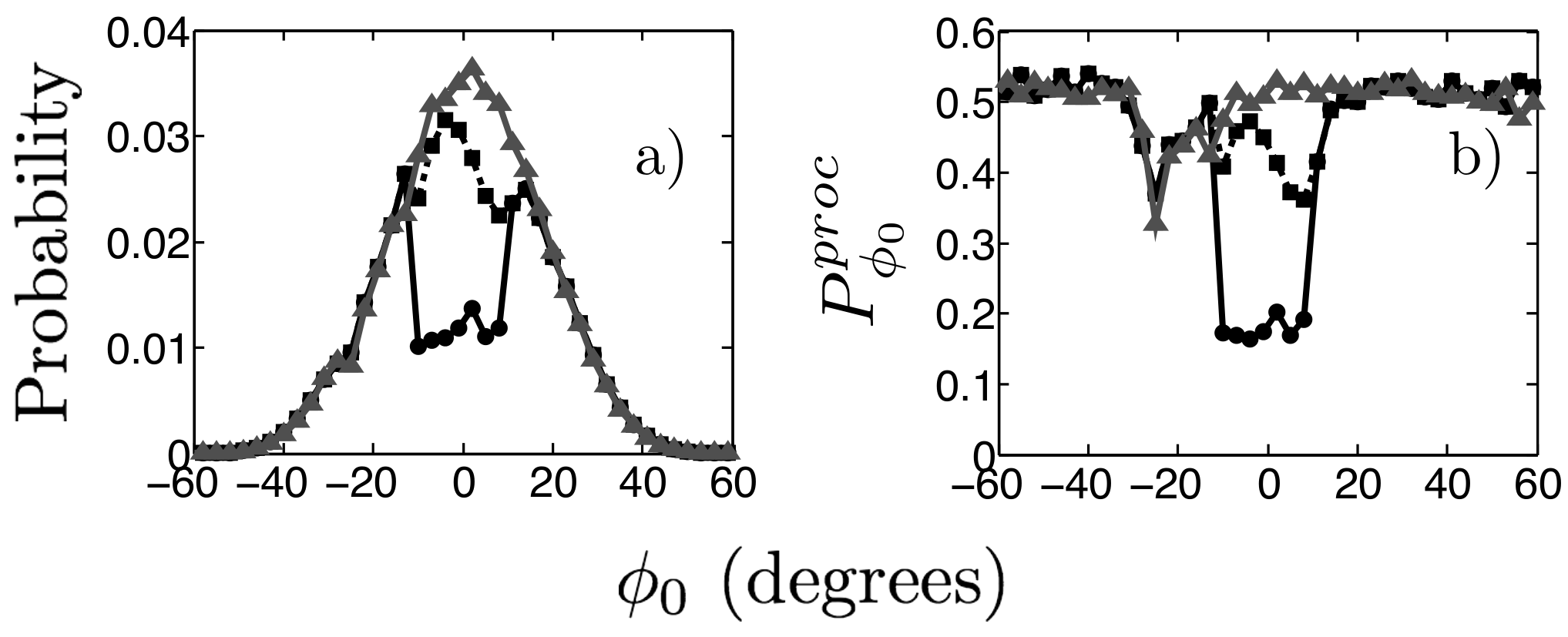
We use both methods and compare the results for the probabilities for double ionization and frustrated ionization for an intensity just below ( W/cm2) and just above ( W/cm2) the threshold intensity for over-the-barrier ionization. One expects that, for each process, the probabilities at these two similar intensities should be very close to each other. In table 1, we show that this condition is satisfied best when using method 2. Moreover, for the above two intensities, in Fig. 1 a) we plot the distribution of the initial phase of the laser field , that is we plot for double ionization events. We find that the distributions for W/cm2 and W/cm2 are more similar when using method 2 rather than method 1 for the over-the-barrier intensity regime. That method 2 is better than method 1 can also be seen in Fig. 1 b) by plotting the probability as a function of . It can be clearly seen that when using method 1 drops sharply in magnitude for corresponding to field strengths in the over-the-barrier-intensity regime. We, therefore, adapt method 2 in our calculations for the over-the-barrier intensity regime.
| I (W/cm2) | |||
|---|---|---|---|
| (Method 1) | (Method 2) | ||
| Double ion. | 49% | 34% | 45% |
| Frustrated ion. | 6.3% | 4.7% | 5.6% |
II.1.1 Exit point of tunneling electron for the below-the-barrier intensity regime
Assuming electron 1 tunnel ionizes with zero momentum along the field direction, we compute the position where electron 1 exits from the field-lowered Coulomb potential using the following equation:
computed at . We solve Eq. (II.1.1) for , the component of along the direction of the field, while setting equal to zero the component of perpendicular to the field; is the first ionization potential, which for is equal to 0.57 a.u. The integral in Eq. (II.1.1) accounts for the screening effect from the bound electron 2. Expressing the wave function of the bound electron 2 in terms of Gaussians we obtain an analytic expression for this integral. is the 1 wave function of at the equilibrium distance of , which we obtain using MOLPRO—a quantum chemistry package [29]. To obtain a relatively simple analytic expression for the integral in Eq. (II.1.1) we expand the wave function in terms of s-symmetry Gaussian functions:
| (4) |
with the contracted s-type functions
| (5) |
and the position vectors of the nuclei. Expanding in s-symmetry Gaussian functions is a very good approximation for the wave function currently under consideration. The final expression for the screening potential due to electron 2 is
where the function is given by
with and the error function [30]. For the current calculation the coefficients , and are obtained from a Hartree-Fock calculation with MOLPRO using the aug-cc-pV5Z basis set. The calculated Hartree-Fock energy for H at the equilibrium distance of H2, is -0.57 a.u. which is in full agreement with the exact value derived in [31].
At this point a brief discussion regarding the exit point is in place. For some simple strongly-driven atoms the exact exit point can be computed using parabolic coordinates [32]. Such computations in terms of parabolic coordinates have been employed in a series of papers, such as [33, 34, 35] to mention just a few. Recently, it was demonstrated that using the exact exit point is necessary to accurately account for the observable momentum of the tunneling electron in attoclock experiments involving single ionization in atoms [36]. For most atoms and molecules, however, it is not possible to compute the exact exit point using parabolic coordinates. Thus, approximations are employed such as the one in the current work. Namely, Eq. (II.1.1) is effectively a 1-d equation where only the potential along the direction of the field is accounted for. That is, we assume that electron 1 tunnels along the direction of the field and, using Eq. (II.1.1), we compute approximately the exit point. For the strong-field phenomena under consideration in our studies, which are double ionization and “frustrated” double ionization, this approximation has proven to be a very good one; our results on “frustrated” double ionization in linearly polarized laser fields [15] are in very good agreement with experimental ones [10].
II.1.2 Exit point of tunneling electron for the over-the-barrier intensity regime
If the instantaneous field strength at the initial phase is larger than the threshold intensity for over-the-barrier ionization, then we assume that electron 1 exits in a direction opposite to the field at a distance [37]; is the coordinate along the laser field direction where the field-lowered Coulomb potential is maximum. In addition, we set the magnitude of the momentum of electron 1, , equal to
| (8) |
The direction of is uniformly distributed in space with the only restriction being that .
II.2 Initial phase space distribution of the nuclei
We take the initial vibrational state of the nuclei to be the ground state of the Morse potential
| (9) |
with the internuclear distance, a.u., a.u., and = 1.4 a.u. (equilibrium distance of H2). The relative momentum of the nuclei satisfies:
| (10) |
where a.u is the vibrational ground state and
| (11) |
where and are the masses of the nuclei. We choose the Wigner distribution of the ground state of the Morse potential [38] to describe the initial phase space distribution of the nuclei. The intensity we consider is high enough to justify restricting the initial distance of the nuclei to [39]. Concerning the relative momentum of the nuclei, , we assign to it a random number uniformly distributed in the interval [0, 10]; for values greater than 10 the Wigner distribution of the state under consideration is essentially zero. After determining the relative momentum, we determine the momenta of the two nuclei [40].
Instead of the Wigner distribution we can use the classical value of the relative momentum, which we find to be equal to 4.3 a.u. from Eq. (10). In addition, we also consider a phase space distribution with the nuclei initially at rest. We find that the Wigner and the two classical distributions yield the same results for the processes under consideration in this work, see Fig. 2.

II.3 Propagation Technique
Next, we describe the technique we follow to propagate the full four-body Hamiltonian in time, i.e. including both electronic and nuclear motion. We present the technique in the context of Coulomb interacting particles that are driven by a laser field. Previously, in [18, 15], we formulated the equations of motion using the global regularization scheme described in [19]. In this latter work, the resulting equations of motion were propagated using the 5th order Runge-Kutta method [21]. In the current work, we use a time-transformed leapfrog propagation technique [20] in conjunction with the Bulirsch-Stoer method [22, 21]. Combining these two techniques has been used successfully to describe gravitational few-body systems [23, 20, 24]. The advantage of the current propagation technique over the one we previously used in [18, 15] is that it is numerically more robust with a smaller propagation error. One reason is that, unlike the technique we previously used, in the current technique the masses do not enter in the time-transformation resulting in a more accurate treatment of many-body systems with large mass ratios [20]. Note that the current technique as well as the technique we previously used in [18, 15] explicitly account for the accurate treatment of the Coulomb singularity during time propagation. This is an essential ingredient of an accurate classical treatment, since classically an electron is allowed to come infinitely close to a nucleus.
II.3.1 Transforming to a new coordinate system
The Hamiltonian for Coulomb interacting particles in the presence of a laser field is given by
| (12) |
where is the charge, is the mass, is the momentum vector and is the position vector of particle and is the laser-field vector. Next, we transform to a new coordinate system that involves the relative coordinate vectors and the corresponding conjugate momenta , which are given by [19]
| (13) |
| (14) |
where and . Expressing and in terms of and we obtain
| (15) |
and
| (16) |
where . Next, we define a fictitious particle for each pair replacing the with the index as follows
| (17) |
for with a total of fictitious particles. Using this notation Eq. (16) takes the form
| (18) |
with and when , otherwise . Expressing the Hamiltonian in Eq. (12) in terms of the relative coordinates and conjugate momenta we obtain
| (19) | |||||
with
| (20) | |||
| (21) | |||
| (22) |
The equations of motion are, then, given by
| (23) | |||||
| (24) |
II.3.2 Time-transformed leapfrog
For close encounters between two particles the Hamiltonian in Eq. (19) is singular. Previously, in [18, 15], this issue was addressed by transforming to regularized coordinates [19]. In the current work, to address the singularity, we use the time-transformed leapfrog method that is described in [20]; we can do so, since in Eq. (24) the derivative expressions are independent of the quantities themselves. In the leapfrog method two sets of first order differential equations are identified. In our case, these two sets correspond to the relative coordinates and the corresponding conjugate momenta . In addition, we consider the time transform [20]; is an arbitrary positive function of the relative position vectors. Introducing a new auxiliary variable the equations of motion take the form , and ; prime denotes the derivate with respect to the new time variable . Instead of using the relation directly, we obtain the value of from the differential equation:
| (25) |
Applying the leapfrog method we now propagate , , and over a time-step as follows: i) we propagate and over half a time-step, ; ii) we propagate and over a time-step using the values of and at half the time step . For each pair of a relative coordinate and the corresponding conjugate momentum the time-transformed leapfrog set of equations take the form:
| (26) |
where the subscripts 0, 1/2, 1 denote the values of the variables at the initial time, at half a time-step and at the end of a time-step. Note that we have such sets of equations, as many as the number of fictitious particles. We choose so that if any of the relative coordinates becomes small (two-body close encounter) then the time-step reduces accordingly:
| (27) |
II.3.3 Bulirsch-Stoer Method
The final step in the integration of the equations of motion, involves incorporating the leapfrog method into the Bulirsch-Stoer method [21, 22]. In this latter method, the propagation over a time step takes place by splitting it into substeps of size . For the propagation over each one of these substeps, we use the time-transformed leapfrog technique. The algorithm we follow to propagate is given by [23, 24]
| (28) |
where . This process of integrating from , to , is repeated with increasing values of until extrapolation to zero time-step, i.e. and for , is achieved with satisfactory error. Using the techniques described above we obtain results similar to those in [15] for H2 when driven by a linearly polarized laser field. The current technique is numerically more robust than the one used in [15] and we, thus, adopt it in what follows.
II.4 Tunneling during propagation
During time propagation, we allow each electron to tunnel at the classical turning points along the field axis using the Wentzel-Kramers-Brillouin (WKB) approximation, for details see [41]. For the transmission probability we use the WKB formula for transmission through a potential barrier [42]
| (29) |
with the potential along the field direction of each electron in the presence of the nuclei and the laser field, which is of the same form as the potential in Eq. (II.1.1) except for the integral term; is the energy of an electron at the time of tunneling, , and and are the classical turning points. We find that accounting for tunneling during time-propagation is necessary in order to accurately describe phenomena related to enhanced ionization during the fragmentation of strongly-driven molecules.
II.5 Identifying Rydberg states in neutral atoms
In what follows, we adopt a Classical Trajectory Monte Carlo (CTMC) method that involves all the techniques discussed in the previous sub-sections. We use this CTMC method to describe the formation of highly excited neutral atoms, through Coulomb explosion, in strongly-driven H2. After propagating the trajectories to the asymptotic limit we select trajectories that produce, H+, a free electron and H∗ (where denotes that the electron is in a quantum state). To identify the trajectories when the electron is captured in an excited state, we first find the classical principal number , where is the total energy of the trapped electron. We, next, assign a quantum number so that the following criterion, which is derived in [43], is satisfied:
| (30) |
III Results
In what follows we consider two laser field intensities, specifically, Wcm2 in the tunneling regime and Wcm2 in the over-the-barrier regime. In Fig. 3 we compute the distribution of the quantum number for and for the two field intensities. We find that the quantum number peaks around 8 in all cases considered. In Fig. 4 we show the energy distribution of the H+ and H∗ fragments for the same two intensities and ellipticities of the laser field. The energy distribution of the H+ and H∗ fragments remains roughly the same as a function of ellipticity while it peaks at a slightly higher value for Wcm2 compared to Wcm2.


Next, we investigate the dependence of the two pathways of formation on the degree of ellipticity of the laser field. These pathways can be separated as to which one of the two ionization steps, i.e., the earlier tunnel ionization of electron 1 or the later tunnel ionization of electron 2 is “frustrated” [15]. In Fig. 5 a) we show pathway A where electron 1 tunnel ionizes, subsequently escaping very quickly. Electron 2, later, tunnel ionizes and quivers in the laser field; however, when the field is turned off, electron 2 does not have enough drift energy to escape and occupies a Rydberg state of the H-atom instead. Hence, in Pathway A the later ionization step is “frustrated”. In Fig. 5 b) we show pathway B where electron 1 tunnel ionizes very quickly, quivering in the field, while electron 2 tunnel ionizes and escapes after a few periods of the laser field. When the laser field is turned off, electron 1 does not have enough energy to escape and remains in a Rydberg state of the H-atom instead, i.e., the earlier ionization step is “frustrated”.
In Fig. 6 we show how the probability of pathway A and B (out of all trajectories) changes with the degree of ellipticity of the laser field. For the smaller intensity of Wcm2, we find that as increases the probability of pathway B drops more sharply than that of A. For instance, for pathway B is 1.6 times more probable than pathway A, while for pathway B is roughly 6 times less probable than A. Thus, for the smaller intensity in the tunneling regime, for pathway B is practically “switched-off” with pathway A prevailing. For the higher intensity of Wcm2, we find that as increases the probability of pathway B drops even more sharply compared to the smaller intensity. For instance, for pathway B is roughly as probable as pathway A, while for pathway B is roughly 25 times less probable than A. Thus, for the higher intensity in the over-the-barrier regime, for pathway B is practically “switched-off”.

The question that naturally arises is why pathway B is more sensitive to the ellipticity of the laser field. Double ionization events where re-collisions prevail are very sensitive to . The reason is that a slight ellipticity of the laser field offsets the electron from the ion roughly by making a re-collision less probable [44]. The sensitivity to ellipticity of our “frustrated” double ionization events for pathway B strongly suggests that two-electron effects in the form of re-collisions underlie pathway B and not pathway A. This explanation is also consistent with pathway B being “switched-off” faster for Wcm2 than for Wcm2: the offset of the re-colliding electron from the ion core increases with increasing intensity of the laser field.
Indeed, in [15] we have provided evidence that one-electron effects prevail in pathway A, while two-electron effects prevail in pathway B. That is, we have shown that in pathway A electron 2 transitions from the ground state of the molecule to a high Rydberg state of the H-atom by gaining energy through a strong interaction with the laser field. This gain of energy resembles enhanced ionization in [7]. We have also provided evidence that in pathway B electron 2 gains energy to ionize mainly through two-electron effects resembling Delayed NSDI (non-sequential double ionization) which is a major pathway of double electron escape (also referred to as re-collision-induced excitation with subsequent field ionization, RESI [45]). In Delayed NSDI (weak re-collision) the re-colliding electron returns to the core close to a zero of the field, transfers energy to the second electron and one electron escapes with a delay after re-collision. For pathway B the electron-electron correlation is in the form of “frustrated” delayed NSDI since one electron eventually does not escape. From the above, it follows that the dependence of the probability of pathways A and B on (Fig. 6) provides strong support that re-collisions underlie pathway B.
Pathway A also decreases with ellipticity, even though pathway A is less sensitive to ellipticity compared to pathway B. To understand this decrease we consider the change in momentum, due to the laser field, of the electron that tunnel ionizes in pathway A, i.e. of electron 2. This change is roughly , where is the time of tunnel ionization and . Moreover, since tunnel ionization takes place mostly around a maximum of the laser field, the change in momentum of electron 2 reduces to . Thus, with increasing ellipticity the momentum of electron 2 increases. As a result “frustrated” double ionization events are converted to double ionization events, accounting for the decrease with ellipticity of the probability of pathway A.
Fig. 6 shows that two-electron effects are essentially “switched-off” in formation for for an intensity Wcm2 and for for an intensity Wcm2 with pathway A prevailing. This prevalence of one-electron effects with increasing is also evident in the observable momentum space of the escaping electron. In Fig. 7 we plot the total x-z momentum distribution of the escaping electron for ellipticities 0 and 0.45 for the two laser field intensities currently under consideration. The total 2-d distributions account for both pathways and all initial tunneling directions of electron 1. For (Fig. 7 a) and c)) the traces of both pathways A and B (Fig. 6) are present in the 2-d momentum distributions. The trace of pathway B is the large spread in momentum [15] which is mostly due to the strong interaction of electron 2 with the Coulomb potential [46]. However, for larger values of this large spread disappears, see Fig. 7 b) and d); this is a clear signature of the prevalence of pathway A. Note that with increasing ellipticity the highest momentum along the x-axis increases. This is expected since the maximum change in momentum along the x-axis, due to the laser field, is approximately given by . We note that the 2-d momentum distributions for the higher intensity reach higher values of momentum in than for the lower intensity. The reason, most probably, is that while in the tunneling regime electron 1 tunnel ionizes at time zero with zero velocity along the direction of the laser field, in the over-the-barrier regime electron 1 tunnels with non zero velocity.
Moreover, for larger values of , see Fig. 7 b) and d), we obtain an asymmetric two-lobe momentum distribution. This asymmetry, first observed in [47], has sparked a lot of studies in single ionization of atoms in elliptical fields. It has been, mainly, attributed to the effect of the Coulomb potential [48]. Since our 3-d semiclassical model fully accounts for the Coulomb potential the asymmetry in the momentum distribution is also evident in our results in Fig. 7 b) and c). Besides the current study, studies of this asymmetry for molecular systems are few; they include a theoretical one of strongly-driven [37] and an experimental one on double ionization of [49]. Our results for formation in Fig. 7 b) and d) show that with increasing the two-lobe structure tends to align closer to the minor axis of the field (x-axis in our case) [49, 37].

Finally, we briefly discuss the sites electron 2 tunnel ionizes from. Specifically, we consider the combined potential of electron 2 in the presence of the two nuclei and the laser field along the direction of the laser field (tunneling direction). Our results indicate that when electron 2 tunnel ionizes the inter-nuclear distances range from intermediate to large. For these distances and at times close to extrema of the field we find that the potential of electron 2 along the direction of the field has either a double or a single-well. For the double-well an inner barrier is present such that the potential of electron 2 is higher in one well (up-field) compared to the other well (low-field) (as is the case for enhanced ionization [7, 6, 8]). The tunnel ionization sites are thus an up-field, low-field and a single-well, see Fig. 8. We consider ellipticities up to 0.45. For Wcm2 we find that, out of all H∗ formation events, electron 2 tunnel ionizes from an up-field well in 85% of the cases while from a low-field or a single-well in 10% of the cases. For Wcm2, we find that electron 2 again mostly tunnel ionizes from an up-field well, however, there is an increased probability to tunnel ionize from a low-field or a single well compared to the lower intensity.

IV Conclusions
We have presented a toolkit for semiclassical computations of strongly-driven molecules. This toolkit includes the formulation of the probabilities of strong-field phenomena in a transparent way. This formulation allowed us to identify an electronic initial phase space distribution for the over-the-barrier intensity regime that works better than previous ones. However, more work is needed to formulate more accurate initial phase space distributions for the electronic degrees of freedom in the over-the-barrier regime. This toolkit also includes a 3-dimensional method for time-propagation that fully accounts for the Coulomb singularity. This 3-d method combines the time-transformed leapfrog propagation technique and the Bulirsch-Stoer method and has been previously developed in the context of celestial mechanics. In the current work, we adopt this technique to strongly-driven systems. Another important element of this toolkit is allowing for tunneling during propagation, that is, the time-propagation is not classical. We find that the latter is necessary in order to accurately describe phenomena associated with enhanced ionization in the fragmentation of strongly-driven molecules. In the current work, using this toolkit, we elucidated the interplay of the electronic and nuclear dynamics in formation during the break-up of strongly-driven by elliptical laser fields. We find that with increasing ellipticity we “switch-off” two-electron effects. That is, we find that pathway A, which is similar to a “frustrated” enhanced ionization process, prevails. Moreover, we have shown that the observable momentum space of the escaping electron clearly bears the imprints of one-electron effects with increasing ellipticity.
Acknowledgments. A.E. acknowledges helpful discussions with Dr. Andre Staudte and support from the EPSRC grants no. H0031771 and J0171831 and the use of the computational resources of Legion at UCL.
Appendix A Ionization rate
For both the below- and the over-the-barrier intensity regimes we use a semiclassical formula for the tunneling rate that was derived in [28]
| (31) |
where is the instantaneous field strength, is the angle between the laser field and the z-axis in the molecular frame, , and is the asymptotic charge. For H2 the asymptotic charge is equal to one. The coefficient is obtained by fitting the Dyson orbital to the following asymptotic form of the wave function
| (32) |
The Dyson orbital [50] is the overlap integral of the two-electron wave function of the molecule with the one-electron wave function of the molecular ion; for the current work the overlap integral is that of the ground state of with the 1 state of computed at the equilibrium distance of . We derive both wave functions with the Hartree-Fock method, using MOLPRO [29]. For H2 the Hartree-Fock energy obtained is -1.134 a.u., which has a 3.5% relative difference from the experimental value of -1.175 a.u. [51].

The function depends on the molecular orbital the electron occupies before tunneling. For H2 the electron occupies a orbital [52],which we can approximately express as a LCAO of two 1s orbitals
| (33) |
Taking the asymptotic expansion for , we derive an expression for
| (34) |
with the distance between the nuclei. An alternative expression is provided in [53]
| (35) |
We find that both expressions give similar results for the tunneling rate. After fitting the Dyson orbital in the interval a.u. and we find and for . The interval was chosen so that for a.u., the Coulomb potential corresponding to the H molecular ion has effectively the form of a one-center Coulomb potential, i.e. ; the upper limit was chosen so that for a.u. the Dyson orbital is practically zero.
As discussed in [28] (shown also here for completeness), the function is given by
where
| (37) | |||
with , , , , and the first and second order partial derivatives of with respect to and , calculated at and . The ionization rate we obtain using Eq. (31) is in very good agreement with the ones obtained in [54, 55], see Fig. 9.
References
- [1] A. Giusti-Suzor, X. He, O. Atabek, and F. H. Mies, Phys. Rev. Lett. 64, 515 (1990).
- [2] A. Zavriyev, P. H. Bucksbaum, H. G. Muller, and D. W. Schumacher, Phys. Rev. A 42, 5500 (1990).
- [3] A. Staudte, C. L. Cocke, M. H. Prior, A. Belkacem, C. Ray, H. W. Chong, T. E. Glover, R. W. Schoenlein, and U. Saalmann, Phys. Rev. A 65, 020703 (R) (2002).
- [4] H. Sakai, J. J. Larsen, I. Wendt-Larsen, J. Olesen, P. B. Corkum, and H. Stapelfeldt, Phys. Rev. A 67, 063404 (2003).
- [5] A. S. Alnaser, T. Osipov, E. P. Benis, A. Wech, B. Shan, C. L. Cocke, X. M. Tong, and C. D. Lin, Phys. Rev. Lett. 91, 163002 (2003).
- [6] H. Niikura, F. Légaré, R. Hasbani, A. D. Bandrauk, M. Yu. Ivanov, D. M. Villeneuve, and P. B. Corkum, Nature 417, 917 (2002).
- [7] T. Zuo and A. D. Bandrauk, Phys. Rev. A 52, R2511 (1995); T. Seideman, M. Yu. Ivanov, and P. B. Corkum, Phys. Rev. Lett. 75, 2819 (1995); D. M. Villeneuve, M. Yu. Ivanov, and P. B. Corkum, Phys. Rev. A 54, 736 (1996); E. Dehghanian, A. D. Bandrauk, and G. Lagmago Kamta, ibid 81, 061403 (2010).
- [8] J. Wu, M. Meckel, L.Ph.H. Schmidt, M. Kunitski, S. Voss, H. Sann, H. Kim, T. Jahnke, A. Czasch, and R. Dörner, Nature Comm. 3 1113 (2012).
- [9] M. Meckel, D. Comtois, D. Zeidler, A. Staudte, D. Pavičić, H. C. Bandulet, H. Pépin, J. C. Kieffer, R. Dörner, D. M. Villeneuve, and P. B. Corkum, Science 320, 1478 (2008).
- [10] B. Manschwetus, T. Nubbemeyer, K. Gorling, G. Steinmeyer, U. Eichmann, H. Rottke, and W. Sandner, Phys. Rev. Lett 102, 113002 (2009).
- [11] T. Nubbemeyer, K. Gorling, A. Saenz, U. Eichmann, and W. Sandner, Phys. Rev. Lett. 101, 233001 (2008).
- [12] T. Nubbemeyer, U. Eichmann, and W. Sandner, J. Phys. B 42, 134010 (2009); B. Manschwetus, H. Rottke, G. Steinmeyer, L. Foucar, A. Czasch, H. Schmidt-Böcking, and W. Sandner, Phys. Rev. A 82, 013413 (2010); B. Ulrich, A. Vredenborg, A. Malakzadeh, M. Meckel, K. Cole, M. Smolarski, Z. Chang, T. Jahnke, and R. Dörner, Phys. Rev. A 82, 013412 (2010).
- [13] J. McKenna, A.M. Sayler, B. Gaire, N. G. Kling, B. D. Esry, K. D. Carnes, and I. Ben-Itzhak, New Journal of Physics 14, 103029 (2012).
- [14] J. Wu, A. Vredenborg, B. Ullrich, L. Ph. H. Schmidt, M. Meckel, S. Voss, H. Sann, H. Kim, T. Jahnke, and R. Dörner, Phys. Rev. Lett 107, 043003 (2011).
- [15] A. Emmanouilidou, C. Lazarou, A. Staudte, and U. Eichmann, Phys. Rev. A 85, 011402 (R) (2012).
- [16] J. Liu, D. F. Ye, J. Chen, and X. Liu, Phys. Rev. Lett. 99, 013003 (2007).
- [17] D. F. Ye, J. Chen, and J. Liu, Phy. Rev. A. 77, 013403 (2008).
- [18] A. Emmanouilidou and A. Staudte, Phys. Rev. A 80, 053415 (2009).
- [19] D. C. Heggie, Celestial Mechanics 10, 217 (1974).
- [20] S. Mikkola and S. Aarseth, Celestial Mechanics and Dynamical Astronomy 84, 343 (2002).
- [21] W. H. Press, S. A. Teukolsky, W. T. Vetterling and B. P. Flannery, Numerical Recipes, Cambridge University Press (2007).
- [22] R. Bulirsch and J. Stoer, Num. Math 8, 1-13 (1966).
- [23] S. Mikkola and K. Tanikawa, Monthly Notices of the Royal Astronomical Society 310, 745 (1999).
- [24] S. Mikkola and K. Tanikawa, New Astronomy 20, 38 (2013).
- [25] X. Hao, G. Wang, X. Jia, W. Li, J. Liu, and J. Chen, Phys. Rev. A 80, 023408 (2009).
- [26] L. Fechner, N. Camus, J. Ullrich, T. Pfeifer, and R. Moshammer Phys. Rev. Lett. 112, 213001 (2014).
- [27] L. Meng, C. O. Reinhold, and R. E. Olson, Phys. Rev. A 40, 3637 (1989).
- [28] R. Murray, M. Spanner, S. Patchkovskii, and M. Yu. Ivanov, Phys. Rev. Lett. 106, 173001 (2011).
- [29] H.-J. Werner P. J. Knowles, G. Knizia, F. R. Manby, M. Schütz, et al., Molpro, version 2012.1, a package of ab initio programs (2012), see http://www.molpro.net.
- [30] M. Abramowitz and I. A. Stegun, Handbook of mathematical functions, Dover Publications, New York (1965).
- [31] H. Wind, J. Chem. Phys. 42, 2371 (1965).
- [32] L. D. Landau and E. M. Lifschitz, Quantum Mechanics Nonrelativistic Theory, 2nd ed., Pergamon, Oxford (1965).
- [33] B. Hu, J. Liu, and S. G. Chen, Phys. Lett. A 236, 533 (1997).
- [34] L. B. Fu, J. Liu, J. Chen, and S. G. Chen, Phys. Rev. A 63, 043416 (2001); L.B. Fu, J. Liu, and S. G. Chen Phys. Rev. A 65, 021406 (2002).
- [35] A. Emmanouilidou, Phys. Rev. A 78, 023411 (2008).
- [36] A. N. Pfeiffer, C. Cirelli, M. Smolarski, D. Dimitrovski, M. Abu-samha, L. B. Madsen, and U. Keller, Nature Phys. 8, 76 (2012).
- [37] K. Doblhoff-Dier, K. I. Dimitriou, André Staudte, and S. Gräfe, Phys. Rev. A 88, 033411 (2013).
- [38] A. Frank, A. L. Rivera, and K. B. Wolf, Phys. Rev. A 61, 054102 (2000).
- [39] A. Saenz, Phys. Rev. A 61, 051402 (R) (2000).
- [40] H. Goldstein, Classical Mechaniss, Addison-Wesley (1980).
- [41] J. S. Cohen, Phys. Rev. A 64, 043412 (2000).
- [42] E. Merzbacher, Quantum Mechanics (Willey, New York, 1998), 3rd ed.
- [43] R. L. Becker and A. D. MacKellar, J. Phys. B 17, 3923 (1984).
- [44] P. Dietrich, N. H. Burnett, M. Ivanov, and P. B. Corkum, Phys. Rev. A 50, 3585 (R) (1994).
- [45] R. Kopold, W. Becker, H. Rottke, and W. Sandner, Phys. Rev. Lett. 85, 3781 (2000); B. Feuerstein, R. Moshammer, D. Fischer, A. Dorn, C. D. Schröter, J. Deipenwisch, J. R. Crespo Lopez-Urrutia, C. Höhr, P. Neumayer, J. Ullrich, H. Rottke, C. Trump, M. Wittmann, G. Korn, and W. Sandner, Phys. Rev. Lett. 87, 043003 (2001).
- [46] D. Comtois, D. Zeidler, H. Pépin, J. C. Kieffer, D. M. Villeneuve, and P. B. Corkum, J. Phys. B 38, 1923 (2005).
- [47] M. Bashkansky, P. H. Bucksbaum, and D. W. Schumacher, Phys. Rev. Lett. 60, 2458 (1988).
- [48] S. P. Goreslavski, G. G. Paulus, S. V. Popruzhenko, and N. I. Shvetsov-Shilovski, Phys. Rev. Lett. 93, 233002 (2004).
- [49] M Spanner, S. Gräfe, S. Chelkowski, D Pavičić, M. Meckel, D. Zeidler, A. B. Bardon, B. Ulrich, A. D. Bandrauk, D. M. Villeneuve, R. Dörner, P. B. Corkum, and A. Staudte, J. Phys. B 45, 194011 (2012).
- [50] S. Patchkovskii, Z. Zhao, T. Brabec, and D. M. Vileneuve, J. Chem. Phys. 126, 114306 (2007).
- [51] K. P. Huber and G. Herzberg “Molecular spectra and molecular structure vol. IV: Constants of Diatomic Molecules”, Van Nostrand-Reinhold Company (1979).
- [52] I. N. Levine, Quantum Chemistry, Prentice Hall, New Jersey, 5th ed. (2000).
- [53] A. A. Radzig and B. M. Smirnov, Reference data, on atoms, molecules, and ions, Springer-Verlag, Berlin (1985).
- [54] S.-Feng Zhao, C. Jin, A.-Thu Le, T. F. Jiang, and C. D. Lin, Phys. Rev. A 81, 033423 (2010).
- [55] A. Saenz, Phys. Rev. A 66, 063408 (2002).