Distributional Analysis for
Model Predictive Deferrable Load Control
Abstract
Deferrable load control is essential for handling the uncertainties associated with the increasing penetration of renewable generation. Model predictive control has emerged as an effective approach for deferrable load control, and has received considerable attention. Though the average-case performance of model predictive deferrable load control has been analyzed in prior works, the distribution of the performance has been elusive. In this paper, we prove strong concentration results on the load variation obtained by model predictive deferrable load control. These results highlight that the typical performance of model predictive deferrable load control is tightly concentrated around the average-case performance.
I Introduction
The electricity grid is at the brink of change. On the generation side, the penetration of wind and solar in the energy portfolio is on the rise due to environmental concerns. And, on the demand side, many smart appliances and devices with adjustable power consumption levels are entering the market. The combination of these two changes make generation less controllable and load less predictable, which makes the traditional “generation follows load” model of control much more difficult.
Fortunately, while smart devices make demand forecasting more challenging, they also provide an opportunity to mitigate the intermittency of wind and solar generation from the load side by allowing for demand response. There are two major categories of demand response, direct load control (DLC) and price-based demand response. See [1] for a discussion of the contrasts between these approaches.
In this paper we focus on direct load control with the goal of using demand response to reduce variations of the aggregate load. This objective has been studied frequently in the literature, e.g., [2, 3], because reducing the variations of the aggregate load corresponds to minimizing the generation cost of the utilities. In particular, large generators with the smallest marginal costs, e.g., nuclear generators and hydro generators, have limited ramp rates, i.e., their power output cannot be adjusted too quickly. So, if load varies frequently, then it must be balanced by more expensive generators (i.e., “peakers”) that have fast ramp rate. Thus, if the load variation is reduced, then the utility can use the least expensive sources of power generation to satisfy the electricity demand.
I-A Model predictive deferrable load control
There is a growing body of work on direct load control algorithms, which includes both simulation-based evaluations [4, 5, 6] and theoretical performance guarantees [7, 8]. The most commonly proposed framework for algorithm design from this literature is, perhaps, model predictive control.
Model predictive control (MPC) is a classical control algorithm, e.g., see [9] for a survey. MPC can be applied to settings where unknown disturbances to the system are present through the robust control paradigm or the certainty equivalence principle, e.g., see [10, 11, 12]. In the context of direct load control, many variations have been proposed. Scalability and performance in the presence of uncertainty are essential to MPC algorithms for direct load control. At this point, there exist model predictive deferrable load control algorithms that can be fully distributed with guaranteed convergence to optimal deferrable load schedules, e.g., [3].
However, to this point, the evaluation of model predictive deferrable load control has focused primarily on average-case analysis, e.g., [13, 14], or worst-case analysis, e.g., [15, 16]. While such analysis provides important insights, there is still much to learn about the performance of model predictive deferrable load control.
For example, it is likely that an algorithm has good average performance but bad worst case performance, and vice versa. What is really needed is a distributional analysis that tells us about the “typical” performance, which can say, e.g., that the load variation will be less than the desired level 95 percent of the time. But, to this point, no results on the distribution of the load variation under model predictive deferrable load control exist.
I-B Contributions of this paper
The main contribution of this paper is to provide a distributional analysis of the load variation under model predictive deferrable load control. More specifically, we prove sharp concentration results for the load variation arising from model predictive distributed load control.
Our results are derived in the context of a standard formulation of the so-called “optimal deferrable load control” (OLDC) problem, where we adopt the model predictive deferrable load control mechanism in [3] since it can be fully distributed, and average-case analysis suggests that it performs well in environments with uncertain predictions.
However, in Proposition 4, we provide a new worst case analysis which states that this model predictive deferrable load control can be as bad as having no control at all if predictions are adversarial.
Given this context, the main result of the paper is Theorem 1, which proves a Bernstein-type concentration for the load variation under model predictive deferrable load control. This result highlights that the load variation is concentrated around its mean, and therefore the typical performance is tightly concentrated around the average performance. Additionally, the result provides useful performance bounds on, e.g., the 95th percentile.
Finally, in addition to the usefulness of Theorem 1 in the context of deferrable load control, the proof technique we develop may also be useful for understanding the distributional performance of model predictive control in other settings.
II Model
In this paper we consider a standard model for deferrable load control introduced by [17] and then studied in, e.g., [6, 18, 7]. It is a discrete-time model where the time-slot length matches the timescale at which the power grid system operator makes control decisions.
The goal is to flatten the aggregate load over the control horizon . In practice, the control horizon could be a day and a time slot could be on the order of minutes. To formalize the objective of flattening the aggregate load, previous work has tended to focus on minimizing the variation of the load:
| (1) |
where is the aggregate load profile at each time slot.
Importantly, the aggregate load consists of two types. The first type, which is called baseload, includes loads like lighting and heating, and is stochastic and non-controllable. Note that renewable generation like wind and solar can be considered as a negative stochastic and non-controllable load. Denote the baseload by , and note that can be interpreted as the difference between non-deferrable load and renewable generation during each time period.
The second type of load, which is called deferrable load, consists of devices whose power consumption can be controlled by the utility, e.g., pool pumps, dryers, and electric vehicles taking part in direct load control programs [19, 20]. It is the control of these devices that can be used to minimize (1), provided that energy constraints and charging rate constraints are satisfied. To model deferrable load we consider devices indexed , and let denote the power consumption of device at time for and . Further, each device has associated constraints on the power consumption as follows
| (2a) | ||||
| (2b) | ||||
Note that, using the above, arrival and deadline constraints can be specified by setting for before arrival and after deadline. Here we assume that the deferrable loads are continuously adjustable in constraint (2a) and the power loss due to heat dissipation can be ignored in constraint (2b). Similar assumptions are made for EV loads in [3, 19]. Although real appliances may deviate from these assumptions, we keep these simplifying assumptions as a first step towards analyzing MPC load control algorithm in the presence of uncertainty.
Given the previous notation, we can now formally specify the optimal deferrable load control (ODLC) problem that is the focus of this paper. Define for .
| (3) | ||||
| over | ||||
| s.t. | ||||
An important observation is that ODLC is a convex optimization problem, but cannot be solved in real time since the optimal decision at time depends on future information about the baseload and the arrivals of deferrable load. This information is not known exactly, but commonly there do exist predictions of future baseload and deferrable load arrivals. So, in practice such predictions are used for real time control.
Thus, the final component of the model is to specify a model for the predictions. Crucially, prediction errors should grow as prediction is made further into the future. Further, it is likely that errors are correlated, e.g., an underestimate for time slot likely leads to an underestimate for time slot . To capture these issues, [3] has suggested a model based on Weiner filters, and we adopt the same assumptions here.
Specifically, baseload is modeled as a random deviation around its expectation as illustrated in Fig. 1. The process is modeled as a sequence of independent random variables , each with mean 0 and variance , passing through a causal filter with impulse response ( for ), i.e.,
Using the current information, one can update the prediction at time by
| (4) |
Further, deferrable loads are modeled as random arrivals over time. Let be the number of loads that arrive before (or at) time for . Define
as the energy request of deferrable loads that arrive at time . We model the total energy request at each time due to arrival of deferrable loads to be a sequence of independent random variables with mean and variance . Further, let denote the total energy requested after time for .
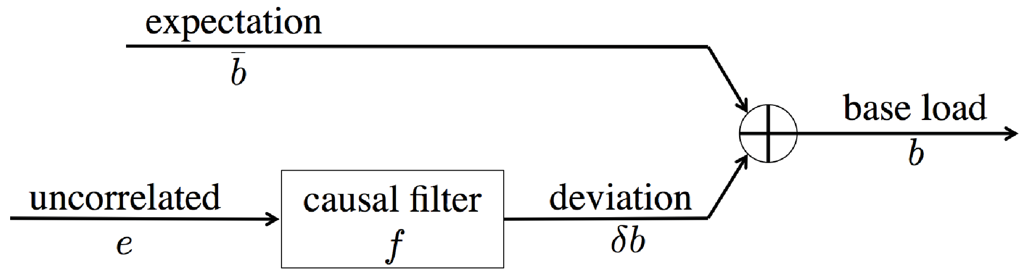
In summary, when attempting to solve ODLC, an algorithm has, at time , the following information: (i) the energy request and power consumption bounds of the present deferrable loads, i.e., , , and for , with for any beyond the consumption deadline; (ii) the expectation of future energy requests; and (iii) the prediction of the non-deferrable load .
III Model predictive deferrable load control
A natural approach for solving the optimal deferrable load control (ODLC) problem described in the previous section is model predictive control, which has been applied in many settings, e.g., see [9] for a survey.
In the context of the ODLC problem, at each time , such an approach uses the updated prediction of baseload and the updated prediction of future energy request to solve an optimization problem over the remainder of the control horizon, and obtains deferrable load profiles for the remainder of the control horizon. Only will be implemented at time , and will be recomputed in the future with more updated predictions.
Interestingly, previous work has found that the optimization problem that is solved should not simply be a truncated version of the ODLC problem as done in receding horizon control (RHC). Instead, [3] suggests introducing a pseudo load to account for the future arrival of deferrable load, and plan for the remainder of the entire horizon, giving rise to the shrinking horizon variant of model predictive control. The introduction of this term allows for strong analytic guarantees on performance [3]. Hence, this is the version of model predictive control we consider in this paper.
Specifically, we consider the model predictive deferrable load control algorithm described in Algorithm 1,
Initialize for ;
At time step ,
where at each time the following optimization problem is solved
| ODLC-t | |||
| over | |||
| s.t. | |||
In this formulation, is the energy to be consumed at or after time , for all and all . Here can be viewed as “pseudo-load” with the constraint that it sums to the expected future energy request . The constraints , are predicted values of maximum and minimum energy request from historical data with . However, if no prediction is available, we can simply set and without affecting the theoretical guarantees of the algorithm.
Importantly, if predictions are exact then Algorithm 1 solves ODLC exactly. Further, prior papers have shown that Algorithm 1 can be run in a completely distributed manner and still ensure (fast) convergence to optimal solutions [3].
For our purposes, the most relevant part of previous studies of Algorithm 1 is that there exists simple characterizations of the solutions to ODLC-, which prove quite useful when analyzing the performance of the algorithm.
Specifically, in cases where there are a large number of deferrable loads, the solutions to ODLC- satisfy a property that is referred to as -valley-filling.
Definition 1.
For any time , a feasible schedule is called -valley-filling, if there exists such that
| (5) |
Proposition 1 ([3]).
At time , a -valley-filling deferrable load schedule, if it exists, solves ODLC-.
This characterization provides a strong basis for the performance analysis of Algorithm 1. To see this, note that if there exists a -valley-filling solution then, besides being optimal, it ensures that the aggregate load satisfies
| (6) |
for . This property tend to be satisfied when the penetration of deferrable load is high, and it gives us a nice structure to analyze the load variance obtained by Algorithm 1. Subsequently, we assume that a -valley-filling exists for each throughout the paper.
IV Performance analysis
The main focus of this paper is the performance analysis of model predictive deferrable load control (Algorithm 1). As discussed, the algorithm has been introduced in [3] followed by the average-case performance analysis. The goal of this paper is to perform a distributional analysis, rather than simply average-case analysis. However, to provide context we first introduce the previous average-case analysis and contrast it with a (novel) worst-case analysis.
IV-A Average-case analysis (previous work)
An average-case analysis of Algorithm 1 was performed in [3]. The following is the main result from that paper.
Proposition 2 ([3]).
If a -valley-filling solution exists for , then the expected load variation obtained by Algorithm 1 is
| (7) |
where for .
Proposition 2 explicitly highlights that as the predictions get precise, i.e., and . More importantly, it follows from Proposition 2 that tends to 0 as time horizon increases, provided that the error correlation decays sufficiently fast with .
This condition is practically relevant since the error correlation usually decays fast with and the time horizon is usually long, which implies that Algorithm 1 should typically have good average case performance.
IV-B Worst-case analysis
The results surveyed above highlight that Algorithm 1 performs well on average; however, it is often important to guarantee more than average case performance. For that reason, many results in the literature focus on worst case, e.g., [21, 22, 12]. While no existing results apply directly to the setting of this paper, we can show that the worst-case performance of Algorithm 1 is quite bad.
To see this, let us consider a setting where the prediction error for generation, , and deferrable load, , have bounded deviations from their means (0 and respectively).
Definition 2.
We say that prediction errors are bounded if there exist and such that, at any time ,
| (8) |
In this situation, it is straightforward to see that the worst case performance of Algorithm 1 can potentially be quite bad. For , define
Proposition 4.
The worst-case performance is achieved when all prediction errors has the maximum magnitude with the appropriate signs—the case where and for all . The proof of this proposition can be found in the technical report [23].
Corollary 1.
Interestingly, the form of Corollary 1 implies that, in the worst-case, Algorithm 1 can be as bad as having no control at all: the time averaged load variation behaves like the worst one step load variation. Meanwhile, recall from Proposition 3 that the average performance as . Hence, while the the load variation has a small mean , it can be quite large in the worst case.
V Distributional analysis
The contrast between the worst-case analysis (Proposition 4) and average-case analysis (Proposition 2) motivates the main goal of this paper — to understand how often the “bad cases,” where takes large values, happen. That is, we want to understand what the typical variations of obtained by Algorithm 1 look like.
V-A Concentration bounds
We start with analyzing the tail probability of . Concretely, our focus is on
which denotes the minimum value such that with probability for . Our main result provides upper bounds on , for large values of , for arbitrary of prediction error distributions.
More specifically, we prove that with high probability, the load variation of Algorithm 1 does not deviate much from its average-case performance, i.e., we prove a concentration result for model predictive deferrable load control.
Theorem 1.
The theorem is proved in the technical report [23]. The proof relies on the technical assumption that -valley-filling profiles exist, which tends to be satisfied with high penetration of deferrable loads. However, in Section V-C, it is shown that the concentration phenomenon still holds in real data traces when this assumption is removed.
Theorem 1 implies that the actual performance of Algorithm 1 does not deviate much from its mean. To illustrate this, consider the following example:
Example 1.
Suppose that the baseload prediction is precise, i.e., . Then the average load variation is
and the tail bound in Theorem 1 can be simplified as
Recall that constant is the variance of and constant is the maximum deviation of from its mean. The above expression shows that, with high probability, is at most a constant times of its mean .
More generally, the quantity controls the decaying speed of the tail bound in (9): the smaller , the faster the tail bound decays in , and the load variation achieved by Algorithm 1 concentrates sharper around its mean . The following corollary highlights that tends to 0 as increases, provided that the error correlation decays fast enough in . Note that the condition on is the same for Corollary 2 and Proposition 3.
Corollary 2.
Under the assumptions of Theorem 1, if the error correlation for some , then as .
A detailed proof of Theorem 1 is included in the technical report [23]. Note that the bound we obtained in Theorem 1 is much sharper than the Markov and Chebyshev bounds for large . This is done by controlling the moment generating function of using the Log-Sobolev inequality similar to the technique used in [24].
V-B Bounds on the variance
To further understand the scale of typical load variation under Algorithm 1, it is useful to also study its variance. In addition, the form of the variance highlights the impact of the tight concentration shown in Theorem 1.
Theorem 2.
To interpret this result, let denote the upper bound on provided in (10). Theorem 10 implies that and scale similarly with .
It immediately follows from the Chebyshev inequality that can only deviate significantly from with a small probability.
Corollary 3.
Under the assumptions in Theorem 10, for ,
| (11) |
While the tail bound (9) in Theorem 1 scales at least exponentially in , the Chebyshev inequality only provides a tail bound (11) that scales inverse quadratically in . Hence for large , (9) provides a much tighter tail bound. However for small values of , the tail bound (11) is usually tighter since the variance is well estimated in (10).
Furthermore, the variance vanishes as expands, provided that decays sufficiently fast as grows, as formally stated in the following corollary.
Corollary 4.
Under the assumptions of Theorem 10, if the error correlation for some , then as .
Note that the condition on parallels that in Proposition 3.
V-C A case study
Theorems 1 and 10 provide theoretical guarantees that the load variance obtained by Algorithm 1 concentrates around its mean, if prediction errors are bounded as in (8) and error correlation decays sufficiently fast (c.f. Corollary 2). Thus, they give the intuition that the expected performance of Algorithm 1 is a useful metric to focus on, and does indeed give an indication of the “typical” performance of the algorithm.
However, our analysis is based on the assumption that a -valley-filling solution exists, which relies on the penetration of deferrable load being high enough. This is a necessary technical assumption for our analysis, and has been used by the previous analysis of Algorithm 1 as well, e.g., [3].
Given this assumption in the analytic results, it is important to understand the robustness of the results to this assumption. To that end, here we provide a case study to demonstrate that this intuition is robust to the -valley-filling assumption.
In our case study, we mimic the setting of [3], where an average-case analysis of Algorithm 1 is performed. In particular, we use 24 hour residential load trace in the Southern California Edison (SCE) service area averaged over the year 2012 and 2013 [25] as the non-deferrable load, and wind power generation data from the Alberta Electric System Operator from 2004 to 2012 [26]. The wind power generation data is scaled so that its average over 9 years corresponds to 30% penetration level, and pick the wind generation of a random day as renewable during each run. We generate random prediction error in baseload and arrival of deferrable load similar to [3].
Given this setting, we simulate 100 instances in each scenario and compare the results with the Theorems 1. The results are shown in Fig. 2 where we plot the cumulative distribution (CDF) of the load variance produced by Algorithm 1 under two different scenarios. Specifically, in Fig. 2(a), we assume the prediction error in wind power generation is , and in Fig. 2(b), we assume the prediction error is . We plot the CDF on the same scale in both plots and additionally show an analytic bound on the confidence interval computed from Theorem 1. For both cases, the results highlight a strong concentration around the mean, and the analytic bound from Theorem 1 is valid despite the fact that the -valley-filling assumption is not satisfied. Further, note that the analytic bound is much tighter when prediction error is small, which coincides the statement of Theorem 1.
VI Conclusion
We have studied a promising algorithm for direct control demand response: model predictive deferrable load control. In particular, we have, for the first time, provided a distributional analysis of the algorithm and shown that the load variance is tightly concentrated around its mean. Thus, our results highlight that the typical performance one should expect to see with model predictive deferrable load control is not-too-different from the average-case analysis. Importantly, the proof technique we develop may be useful for the analysis of model predictive control in more general settings as well.
The main limitation in our analysis (which is also true for the prior stochastic analysis of model predictive deferrable load control) is the assumption that a -valley-filling solution exists. Practically, one can expect this to be satisfied if the penetration of deferrable loads is high; however, relaxing the need for this technical assumption remains an important challenge. Interestingly, the numerical results we report here highlight that one should also expect a tight concentration in the case where a -valley-filling solution does not exist.
References
- [1] M. H. Albadi and E. El-Saadany, “Demand response in electricity markets: An overview,” in Power Engineering Society General Meeting, 2007. IEEE, June 2007, pp. 1–5.
- [2] E. Sortomme, M. Hindi, S. MacPherson, and S. Venkata, “Coordinated charging of plug-in hybrid electric vehicles to minimize distribution system losses,” Smart Grid, IEEE Transactions on, vol. 2, no. 1, pp. 198–205, March 2011.
- [3] L. Gan, A. Wierman, U. Topcu, N. Chen, and S. H. Low, “Real-time deferrable load control: handling the uncertainties of renewable generation,” in Proceedings of the fourth international conference on Future energy systems. ACM, 2013, pp. 113–124.
- [4] S. Acha, T. C. Green, and N. Shah, “Effects of optimised plug-in hybrid vehicle charging strategies on electric distribution network losses,” in Transmission and Distribution Conference and Exposition, 2010 IEEE PES. IEEE, 2010, pp. 1–6.
- [5] K. Mets, T. Verschueren, W. Haerick, C. Develder, and F. De Turck, “Optimizing smart energy control strategies for plug-in hybrid electric vehicle charging,” in Network Operations and Management Symposium Workshops (NOMS Wksps), 2010 IEEE/IFIP. IEEE, 2010, pp. 293–299.
- [6] M. Ilic, J. W. Black, and J. L. Watz, “Potential benefits of implementing load control,” in Power Engineering Society Winter Meeting, 2002. IEEE, vol. 1. IEEE, 2002, pp. 177–182.
- [7] Z. Ma, D. Callaway, and I. Hiskens, “Decentralized charging control for large populations of plug-in electric vehicles,” in Decision and Control (CDC), 2010 49th IEEE Conference on. IEEE, 2010, pp. 206–212.
- [8] L. Gan, U. Topcu, and S. H. Low, “Stochastic distributed protocol for electric vehicle charging with discrete charging rate,” in Power and Energy Society General Meeting, 2012 IEEE. IEEE, 2012, pp. 1–8.
- [9] S. J. Qin and T. A. Badgwell, “A survey of industrial model predictive control technology,” Control engineering practice, vol. 11, no. 7, pp. 733–764, 2003.
- [10] E. F. Camacho and C. B. Alba, Model predictive control. Springer, 2013.
- [11] W. H. Kwon and S. H. Han, Receding horizon control: model predictive control for state models. Springer, 2006.
- [12] A. Bemporad and M. Morari, “Robust model predictive control: A survey,” in Robustness in identification and control. Springer, 1999, pp. 207–226.
- [13] A. J. Conejo, J. M. Morales, and L. Baringo, “Real-time demand response model,” Smart Grid, IEEE Transactions on, vol. 1, no. 3, pp. 236–242, 2010.
- [14] J. Roos and I. Lane, “Industrial power demand response analysis for one-part real-time pricing,” Power Systems, IEEE Transactions on, vol. 13, no. 1, pp. 159–164, 1998.
- [15] S. Chen and L. Tong, “iems for large scale charging of electric vehicles: Architecture and optimal online scheduling,” in Smart Grid Communications (SmartGridComm), 2012 IEEE Third International Conference on. IEEE, 2012, pp. 629–634.
- [16] Q. Li, T. Cui, R. Negi, F. Franchetti, and M. D. Ilic, “On-line decentralized charging of plug-in electric vehicles in power systems,” arXiv preprint arXiv:1106.5063, 2011.
- [17] K.-H. Ng and G. B. Sheble, “Direct load control-a profit-based load management using linear programming,” Power Systems, IEEE Transactions on, vol. 13, no. 2, pp. 688–694, 1998.
- [18] L. Gan, U. Topcu, and S. Low, “Optimal decentralized protocol for electric vehicle charging,” in Decision and Control and European Control Conference (CDC-ECC), 2011 50th IEEE Conference on. IEEE, 2011, pp. 5798–5804.
- [19] K. Clement-Nyns, E. Haesen, and J. Driesen, “The impact of charging plug-in hybrid electric vehicles on a residential distribution grid,” Power Systems, IEEE Transactions on, vol. 25, no. 1, pp. 371–380, Feb 2010.
- [20] M. Pedrasa, T. Spooner, and I. MacGill, “Coordinated scheduling of residential distributed energy resources to optimize smart home energy services,” Smart Grid, IEEE Transactions on, vol. 1, no. 2, pp. 134–143, Sept 2010.
- [21] J. a. Lee and Z. Yu, “Worst-case formulations of model predictive control for systems with bounded parameters,” Automatica, vol. 33, no. 5, pp. 763–781, 1997.
- [22] M. Lin, Z. Liu, A. Wierman, and L. L. Andrew, “Online algorithms for geographical load balancing,” in Green Computing Conference (IGCC), 2012 International. IEEE, 2012, pp. 1–10.
- [23] N. Chen, L. Gan, S. H. Low, and A. Wierman, “Distributional Analysis for Model Predictive Deferrable Load Control,” ArXiv e-prints, Mar. 2014.
- [24] S. Boucheron, G. Lugosi, P. Massart et al., “On concentration of self-bounding functions,” Electronic Journal of Probability, vol. 14, no. 64, pp. 1884–1899, 2009.
- [25] “Southern california edison dynamic load profiles,” https://www.sce.com/wps/portal/home/regulatory/load-profiles, 2013.
- [26] “Alberta eelctric system operator. wind power and alberta internal load data,” http://www.aeso.ca/gridoperations/20544.html, 2012.
- [27] M. Ledoux, “Concentration of measure and logarithmic sobolev inequalities,” in Seminaire de probabilites XXXIII. Springer, 1999, pp. 120–216.
Appendix A Proof of Proposition 4
It has been computed in [3] that the load variance obtained by Algorithm 1 is composed of two parts:
where
is the variance due to the prediction error on deferrable load and
is the variance due to the prediction error on baseload. Now we compute the worst-case and under the bounded prediction error assumption (8).
We start with computing the worst-case . Let for , then
The first term
where for . Let the matrix be given by
for , i.e.,
then
where the vector . When prediction error is bounded as in (8), one has for all , and therefore
and the equality is attained if and only if for all , or for all . Finally, we simplify the worst-case expression of as follows:
We proceed to compute the worst-case . Using the same derivation, it can be computed that
where
It follows that
and that the equality is attained if and only if for all , or for all . Finally, we simplify the worst-case expression of as follows:
To summarize, the worst-case load variance obtained by Algorithm 1 is
Appendix B Proof of Theorem 1
The theorem relies on a variant of the Log-Sobolev inequality provided in the following lemma.
Lemma 1 (Theorem 3.2, [27]).
Let be convex and be supported on , then
| (12) |
If is further “self-bounded”, then its tail probability can be bounded as in the following lemma.
Lemma 2.
Let be convex and be supported on . If and satisfies the following self-bounding property
| (13) |
then the tail probability of can be bound as
| (14) |
Proof.
Denote the moment generating function of by
The function is convex, and therefore it follows from Lemma 1 that
According to the self-bounding property (13), one has
Divide both sides by to get
Integrate both sides from 0 to to get
for . Noting that and , one has
and therefore
| (15) |
for . We can bound the tail probability with the control (15) over the moment generating function .
In particular, one has
for . Choose to get
∎
Proof of Theorem 1.
It has been computed in [3] that the load variance obtained by Algorithm 1 is composed of two parts:
where
is the variance due to the prediction error on deferrable load and
is the variance due to the prediction error on baseload.
Let for , then
where the matrix is given by
Similarly, the variance due to the prediction error on baseload can be written as
where the matrix is given by
for . Therefore, the load variance
where
Define a centered random variable
and note that the function is convex. Let be the maximum eigenvalue of , then
According to the bounded prediction error assumption (8), one has componentwise. Then, apply Lemma 14 to the random variable to obtain
for , i.e.,
for . Finally, let , , and , the largest eigenvalue of can be bounded above as
The last equality is because
and
.
Appendix C Proof of Theorem 10
The derivation of the theorem is based on the following two lemma, which separates the cases when there is only one type of prediction error.
Lemma 3.
If there is no prediction error in the base load, then the variance of the performance of Algorithm 1 is bounded by
| (16) |
Lemma 4.
If there is no prediction error in the deferrable load, then the variance of the performance of Algorithm 1 is bounded by
| (17) |
Firstly we will prove Lemma 16, where we only consider prediction error in deferrable load.
Proof of Lemma 16.
Let , then is centered, with variance . Let . From the results in [3] Lemma 1, we have
Define an auxilary matrix such that
Then we have
Hence is a convex function, by convex Poincaré inequality, we have
| (18) |
Whereas
∎
Next we proof lemma 17 the case where we only consider the prediction error in the base load.
Proof of Lemma 17.
Let , when there is no prediction error in the deferrable load arrival, we have
If we define an auxilary matrix such that
Then we have
Hence is a convex function in . By similar argument as Lemma 16
| (19) |
Whereas
∎
Next, we bring the two results together to get a proof of Theorem 10.
Proof of Theorem 2.
Let be the load variance without prediction error in base load and be the load variance without prediction error in the deferrable load.
By independence of and , the variance of is bounded by
∎