Statistics of the inverse-cascade regime in two-dimensional magnetohydrodynamic turbulence
Abstract
We present a detailed direct numerical simulation of statistically steady, homogeneous, isotropic, two-dimensional magnetohydrodynamic (2D MHD) turbulence. Our study concentrates on the inverse cascade of the magnetic vector potential. We examine the dependence of the statistical properties of such turbulence on dissipation and friction coefficients. We extend earlier work significantly by calculating fluid and magnetic spectra, probability distribution functions (PDFs) of the velocity, magnetic, vorticity, current, stream-function, and magnetic-vector-potential fields and their increments. We quantify the deviations of these PDFs from Gaussian ones by computing their flatnesses and hyperflatnesses. We also present PDFs of the Okubo-Weiss parameter, which distinguishes between vortical and extensional flow regions, and its magnetic analog. We show that the hyperflatnesses of PDFs of the increments of the stream-function and the magnetic vector potential exhibit significant scale dependence and we examine the implication of this for the multiscaling of structure functions. We compare our results with those of earlier studies.
Keywords:
MHD, turbulence, multiscaling , inverse cascadepacs
47.27.-i, 47.27.ek, 47.27.er, 47.27.GsI Introduction
The energy spectrum describes the distribution of energy over the wave-number () scales in a turbulent fluid; it is, therefore, an important statistical measure of the characteristics of fluid turbulence. In three-dimensional (3D) fluid turbulence, energy, injected at , cascades down to small length scales (), because of the nonlinearities in the system, and leads to the scaling form , in the inertial range , where and the Kolmogorov dissipation length scale is ; at the level of Kolmogorov’s [1, 2] phenomenological theory (K41), . This Richardson forward cascade of energy, from large to small length scales, continues until the length scale , at which point viscous dissipation becomes significant [2, 3] and falls very rapidly for .
In two-dimensional (2D), statistically steady turbulence, the Richardson forward cascade is replaced by two cascades, one forward and the other inverse [2, 4, 5, 6, 7, 11, 9, 10], because of the conservation of energy and enstrophy in the unforced, inviscid limit. In the forward-cascade regime, enstrophy cascades from to larger values of and leads to , where depends on the friction on the 2D fluid film (if there is no friction, ); by contrast, in the inverse-cascade regime, energy cascades from to smaller values of , which leads to the formation of large vortices, whose size is limited, finally, by the friction [11, 9, 10, 12, 13, 14]. Direct numerical simulations (DNSs) have been used to study the two cascades in 2D fluid turbulence in great detail [15].
Inverse energy cascades have been found and investigated in other turbulent systems, such as quasi-geostrophic flows [16, 17] and turbulence in fluid films with polymer additives [18]. It has also been noted that quantities other than the energy can show inverse cascades; examples include the inverse cascade of magnetic helicity in three-dimensional (3D) MHD turbulence [19, 20] and its analog in 2D MHD turbulence [21]. The 3D MHD equations conserve the energy , cross helicity, and magnetic helicity in the inviscid, unforced case; when viscosity and magnetic diffusivity are included, forced 3D MHD turbulence displays a nonequilibrium statistically steady state in which the magnetic helicity displays an inverse cascade, from the forcing length scale to larger scales, whereas the energy and cross helicity display forward cascades [22, 19]. The 2D MHD analog of the magnetic helicity is , where is the 2D scalar analog of the 3D magnetic vector potential [23]. The inverse cascade in turbulent MHD is very important in the formation of large-scale structures in astrophysical plasmas [20, 24].
To provide some background for our study, we begin with dimensional predictions [21, 25] for the fluid- and magnetic-energy spectra, and , respectively, in the 2D MHD inverse-cascade regime, which we have described above. The dimensions (indicated by square brackets and expressed as powers of length and time ) of various quantities are given below (velocity and magnetic fields have the same units in the standard formulation of MHD [26, 27]):
| (1) |
here, and are, respectively, dissipation rates per unit time for and , and the arguments denote spatial fourier transforms. displays an inverse cascade, so we can make a Kolmogorov-type ansatz [26, 1, 2, 11] for its spectrum, namely, in the inverse-cascade region, should not depend on viscosity, magnetic diffusivity, and friction. Therefore, we write
| (2) |
and then dimensional analysis (Eq. 1) requires
| (3) |
from which we find and and , i.e.,
| (4) |
To obtain the scaling form for , we must make an additional assumption. One such assumption [25] is that the nonlinear terms in the velocity equation in 2D MHD (see below) must balance each other in the inverse-cascade regime; this assumption implies . It has been suggested [21] that this result is valid only in the forward-cascade parts of these energy spectra, because the large-scale part of the magnetic field leads to an Alfvén-type effect, which yields, in turn, a strong coupling between small-scale velocity and magnetic fields and implies, thereby, that ; Ref. [21] goes on to suggest that this effect may not operate in the inverse-cascade regime in 2D MHD. Our study has been designed to explore, among other issues, the scaling forms of such spectra in this regime.
We build on earlier studies of inverse cascades in homogeneous, isotropic, and statistically steady MHD turbulence, in both 3D [19] and 2D [21], by carrying out extensive direct numerical simulations (DNSs) of the forced 2D MHD equations, with friction, and forcing that yields a substantial spectral regime in which there is a substantial inverse-cascade region in the spectrum for . We investigate two cases R1, with a finite, positive friction, and R2, with zero friction. Our study yields a variety of interesting and unforeseen results.
The most remarkable result of our study is that the runs R1 and R2 yield quantitatively different statistical properties. In particular, run R1 yields fluid- and magnetic-energy spectra whose scaling forms in the inverse-cascade regime are, respectively, consistent with and ; by contrast, run R2 yields energy spectra that are consistent with and . Furthermore, we find that, in both runs R1 and R2, the PDFs of , , , and (the fluid stream function) are close to Gaussian; we characterize mild deviations from Gaussian forms by calculating the kurtoses for these PDFs. The PDFs of field increments, such as , are also predominantly Gaussian, but their hyperflatnesses , which depend on the length scale , show deviations from the Gaussian value of 15, especially for the increments and . The angle between and is and that between and is . We obtain the PDFs of these angles and show therefrom that, in both runs R1 and R2, (a) and are perfectly aligned or anti-aligned, with equal probability, and (b) the PDF of is symmetrical about a minima at and attains its highest values at . We obtain the Okubo-Weiss parameter , which is positive (negative) in regions where the fluid flow is vortical (extensional), and its magnetic analog ; we then obtain PDFs of and and also their joint PDF; and we show that they are qualitatively similar for runs R1 and R2; in particular, the PDFs have a cusp at the origin and tails that we fit to exponential forms. We also explore the scaling and possible multiscaling of structure functions of field increments.
The remaining part of this paper is organized as follows. Section II contains a description of equations of 2D MHD, the quantities we calculate, and the numerical methods we use. In Section III we present our results. Section IV contains our conclusions and a discussion of our results.
II model and numerical methods
The 2D MHD equations can be written as
where , the magnetic field, and , the velocity field, are related to the 2D analog of the magnetic vector potential and the stream function as follows: and , where is the unit vector normal to our 2D simulation domain. The current density and vorticity fields are, respectively, and . In this form, the 2D MHD equations satisfy the incompressibility condition and . The order of the dissipativity is , the coefficients of friction in the two equations are and , respectively, and and are, respectively, the kinematic viscosity and magnetic diffusivity; and are the forcing terms. We carry out two DNSs of these equations; the first DNS (R1) has hyperviscosity and hyperdiffusivity with , which allow us to obtain large inertial ranges in energy spectra; and the second DNS (R2) has conventional viscosity and diffusivity with ; the other parameters for these runs are given in Table 1. In the DNS R2, , so the inverse cascade in leads to an accumulation of magnetic energy at small in the magnetic-energy spectrum (Fig. 1). To control this small- accumulation and to obtain a statistically steady state, we use but in DNS R1. Our DNSs use a standard pseudo-spectral method [28, 21, 13] in a two-dimensional, square simulation domain with side and periodic boundary conditions in both and directions; we remove aliasing errors by using a two-third dealiasing method. For time marching, we use a second-order, Runge-Kutta method.
| Runs | |||||||||||||||
|---|---|---|---|---|---|---|---|---|---|---|---|---|---|---|---|
| R1 | |||||||||||||||
| R2 |
We obtain a statistically steady state by the following procedure: We first carry out a DNS of Eqs. () with , i.e., no forcing, and an initial condition , , where and are independent random phases distributed uniformly on the interval . We then evolve the system until we obtain a peak in the energy-dissipation rate; this signals that the energy in the low- modes has cascaded down to high- modes. At this time, we start forcing the system at a large value of , in order to obtain a clear, inverse-cascade regime. We use the following forcing terms:
| (6) |
We now allow the system to reach a statistically steady state, maintain it in this state for , where is the box-size eddy-turnover time, and then collect data for an averaging time (see Table 1) for the statistical properties we study.
In addition to the spatiotemporal evolution of and , we obtain , and . The fluid Reynolds number is , its magnetic analog is , the root-mean-square velocity is , the effective viscosity and magnetic diffusivity are, respectively,
| (7) |
the box-size eddy turnover time is , and the kinetic- and magnetic-energy spectra are and , respectively. We also calculate the fluid Okubo-Weiss parameter [29, 30, 13]
| (8) |
For a fluid, in the inviscid, unforced case without friction, the sign of can be used to distinguish between vortical and extensional regions of the flow. In particular, the flow is vortical, if , and it is extensional, if . This criterion works well even in the presence of viscosity, friction, and forcing [13].
It is useful to introduce the magnetic analog of the fluid Okubo-Weiss parameter ; follows from the determinant of the magnetic-field-gradient tensor and can be written as the difference of the squares of the current density and the magnetic strain rate [31]. Thus, we expect that in current-dominated regions, whereas in regions that are dominated by the magnetic strain rate. Specifically, is defined as follows [31]:
| (9) |
We obtain field-increment PDFs and structure functions from and similar equations for , , and . We also calculate similar PDFs for the longitudinal components of the velocity- and magnetic-field increments, i.e., and its magnetic counterpart. The order-, longitudinal structure function of a field is ; when we calculate , we subtract the mean-flow value of from its value at a given point in space, average over (i) a circle of radius , (ii) different, representative origins , and (iii) over independent field configurations, which are separated from each other by one .
III results
We present our results in three subsections. The first subsection (III.1) is devoted to a discussion of the spectra we obtain from runs R1 and R2. The second subsection (III.2) deals with one-point statistics and PDFs. The third subsection (III.3) contains two-point statistics, such as PDFs of field increments and structure functions.
III.1 Spectra
In Fig. 1 we plot various spectra for run R1. Figure 1 (a) shows log-log plots of the kinetic- and magnetic-energy spectra (red curve) and (blue curve), respectively, versus the wave number , with sharp peaks at the energy-injection wave number . For , these spectra display power-law regimes, which are consistent with and , as we can see from the compensated spectra of Fig. 1 (b), where the dashed line indicates the range of (slightly more than a decade from ) over which we obtain these power-law forms. These power laws are cut off at very small values of , because of the friction term in Eq.( ); and the hyperviscous term yields the mild bottleneck maxima [32], which are clearly visible in the compensated spectra (Fig. 1 (b)) close to and to the left of . Figure 1 (c) shows log-log plots of the vorticity (red curve) and current (blue curve) spectra and , respectively, which follow simply from the energy spectra mentioned above. Plots of the stream-function and magnetic-vector-potential spectra (red curve) and (blue curve) are given in Fig. 1 (d).
Figure 3 (a) is the analog, for run R2, of Fig. 1 (a), for run R1. A comparison of the energy spectra in these two figures highlights important differences between our runs R1 and R2. The energy spectra for run R1 do not increase indefinitely as , because of the friction term, whereas those for run R2 do increase, because this run does not use friction. The compensated spectra of Fig. 1 (b) (run R1) show bottleneck maxima, but those of Fig.3 (b) (run R2) do not, because run R1 uses hyperviscosity, but run R2 does not [32].
Another important difference between runs R1 and R2 is that the latter takes a much longer time to reach a statistically steady state than the former. [It has been noted in the context of 2D fluid turbulence [33] that a simulation time of order is required to obtain such a steady state if there is no friction (here is the smallest wave number in the DNS).] This is why the spatial resolution (and, therefore, the extent of the power-law range in the spectrum) of run R2 is lower than that of run R1. In Fig. 2 we plot the total, kinetic, and magnetic energies versus time, for run R2, and the last , to show that we have, indeed, reached a statistically steady state (the total length of this DNS is ). From Figs. 3 (a) and (b) we see that the power-law regimes in these kinetic- and magnetic-energy spectra have scaling forms that are consistent with and . In Figs. 3 (d) we plot the vorticity spectrum and the current density spectrum , and in (e) we plot the spectra of the stream function and magnetic potential and , respectively.
III.2 One-point statistics
In Figs. 4 (a)-(d) we show, for Run R1, PDFs (red curves) of and , respectively, with Gaussian PDFs (blue dashed curves) for comparison. The PDFs of and do not show significant deviations from Gaussian PDFs, but the tails of the PDFs of and lie, respectively, above and below their Gaussian counterparts. We confirm this by obtaining the kurtoses or flatnesses and ; we find and , both of which differ significantly from the Gaussian (superscript ) value . We obtain similar results for run R2.
In Figs. 5 (a) and (b) we present, for run R1, PDFs of the cosines of the angles and between (a) and and (b) and , respectively. These PDFs quantify the degree of alignment between these vectors. From Fig. 5 (a) we see that and , which are perpendicular to the simulation domain and can be viewed as pseudoscalars, are either perfectly aligned or antiparallel. The PDF of Fig. 5 (b) shows that and , which lie in the 2D simulation plane, have a greater tendency to be aligned or antiparallel than to be orthogonal; and the PDF of is symmetrical about its minimum at . We obtain similar results for run R2. For earlier studies of such alignment PDFs we refer the reader to Ref. [34], which invertigates field alignments for decaying 3D and 2D MHD turbulence.
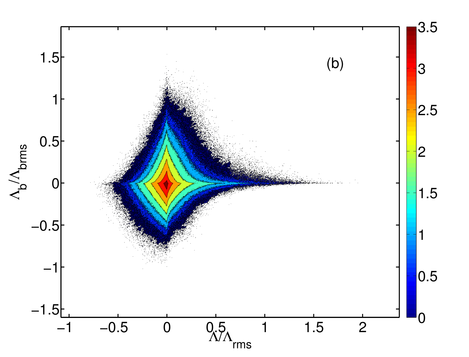
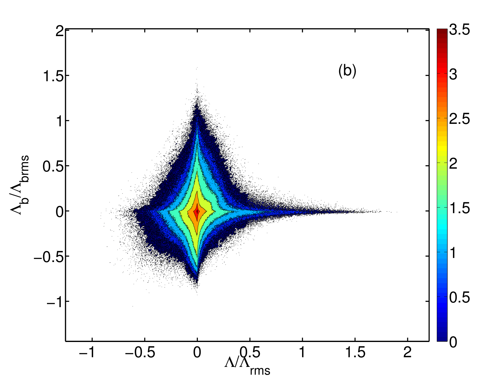
We calculate and by using Eqs. (8) and (9) and then obtain their PDFs and , which are shown, respectively, by red and blue curves in Fig. 6 (a) (for run R1) and Fig. 7 (a) (for run R2). There are two qualitative similarities between and for both runs R1 and R2: all these PDFs show a cusp at or ; and all of them have tails that can be fit to exponentials over the range of values we consider. For runs R1 (subscript ) and R2 (subscript ) we parametrize the left (subscript ) and right (subscript ) tails of these PDFs as follows:
| (10) |
here, the superscripts and denote velocity and magnetic fields. We find , , , and , and , , , and .
We show the joint PDF of and in Figs. 6 (b) and 7 (b), for runs R1 and R2, respectively, by using filled contours (and a logarithmic color scale). The joint PDF can be divided into the following four regions: (1) and , where our 2D MHD flows are dominated by vorticity and current; (2) and , where the flow is dominated by vorticity and magnetic strain rate; (3) and , where the flow is dominated by the fluid strain and the current; (4) and , where the flow is dominated by fluid and magnetic rates of strain. The joint PDF for run R1 (Fig. 6 (b)) is qualitatively similar to its counterpart for R2 (Fig. 7 (b)). These joint PDFs have sharp peaks at and ridges that seperate the four regions mentioned above.
The Okubo-Weiss parameter has been used in several studies [29, 30, 13] of 2D fluid turbulence to distinguish between vortical and elongational regions in the flow. We are not aware of any study of 2D MHD turbulence that uses and to differentiate, explicitly, between various flow topologies. (For studies of similar issues in 3D MHD turbulence, see, e.g., Refs. [35, 36].) We present pseudocolor plots of (left panels of Figs. 8 and 9, for runs R1 and R2, respectively) on which we have overlaid the contours of the stream function ; in these plots we have zoomed into a representative, square region in the simulation domain. (Such plots for 2D fluid turbulence have been given in Ref. [13].) We give similar pseudocolor plots of (right panels of Figs. 8 and 9, for runs R1 and R2, respectively) on which we have overlaid contours of the magnetic potential . From the left panels of Figs. 8 and 9, we see that vortical regions () are associated with centers in the contours of , whereas large-strain-rate regions () correspond to the regions where the contours of have a large curvature. Similarly, the right panels of Figs. 8 and 9 show us that current-dominated regions () are associated with centers in the contours of , whereas large-magnetic-strain-rate regions () correspond to the regions where the contours of have a large curvature. We give pseudocolor plots of and in Figs. 10 (a) and (b) (for run R1) and Figs. 10 (c) and (d) (for run R2), for the complete simulation domain.


III.3 Two-point statistics
In Figs. 11 (a)-(f), we plot PDFs of the field increments (a) , (b) , (c) , (d) , (e) , and (f) , for (red curves) and (green curves). These PDFs lie very close to Gaussian ones, which are shown by dashed blue curves; small, non-Gaussian deviations appear in the PDF tails. To quantify the scale dependence of these deviations, we obtain the hyperflatness for all fields . In the insets of Figs. 11 (a)-(f), we show plots of versus , etc., to demonstrate that, at least up to order , our structure functions are reliable. We present plots versus of the hyperflatnesses of the field increments in the left and right panels of Fig. 12 for (a) (red curve), (blue curve), and (green curve) and (b) (red curve), (blue curve), and (green curve). From these plots we see that, in run R1, and (red curves in Figs. 12 for (a) and (b), respectively) lie slightly above the Gaussian value for , they increase gently for lower values of , indicating an enhancement of small-scale intermittency, and decrease again towards the Gaussian value after going through at maximum at which these hyperflatnesses are . In contrast, and (green curves in Figs. 12 for (a) and (b), respectively) do not show significant scale dependence; the former lies above the Gaussian value, whereas the latter is only a few percent above this. and (blue curves in Figs. 12 for (a) and (b), respectively) also do not show significant scale dependence; the former lies below the Gaussian value, whereas the latter is above this. Given that the spectra for runs R1 and R2 are different, it is not surprising that the scale dependences of the hyperflatnesses are different for these runs too, as we can see by comparing the plots in Figs. 12 (a) and (b), for run R1, with their counterparts in Figs. 12 (c) and (d), for run R2.
Note that there are well-defined, damped oscillations in and , at small values of (these show up especially clearly on the scales of Figs. 12 (c) and (d)). The distance between successive maxima in these oscillations is . Such damped oscillations also appear in plots of structure functions; we show an illustrative plot for in Fig. 13 (a). The origin and form of these oscillations can be understood easily for second-order structure function of field because it is related, via Fourier transformation, to the spectrum . We show this explicitly below for .
We consider homogeneous, isotropic, turbulence, so depends only on , therefore,
| (11) |
where we control the ultra-violet (UV) divergence of the integrals by using a UV cutoff and make the assumption , which is consistent with the spectrum in Fig. 1 for run R1. (For run R2, , so the subsequent steps cannot be carried out analytically; however, the oscillations are more pronounced than they are in the case .) We obtain, finally,
| (12) |
where and , with or , denote, respectively, Bessel and Struve functions [38], which oscillate in a manner that is consistent with the plot in Fig. 13. (a) Similar arguments for the second-order, logitudinal velocity structure function (with in Fig. 1 for run R1) yield
| (13) |
The structure functions for and do not show such oscillations because the Fourier integrals are UV convergent.
The oscillations appear much more clearly in than in because, for large , , whereas . The relative strengths of these oscillations is governed by the ratio of the coefficients of the second terms in and is proportional to , which is large because can be taken to be (this is consistent with the period of oscillations that we see in the inset of Fig. 13 (a)). Thus, we expect the oscillations in to be more conspicuous than their counterparts in . From the spectra presented in subsection III.1, we know that the constants of proportionality, in Eqs. (12) and (13) for and are of the same order of magnitude.
Given the oscillations in and , and the lack of significant scale dependence in the plots of and (Figs. 12 (a)-(d)), we do not expect noticeable multiscaling in vorticity and velocity structure functions in the inverse-cascade range. However, given the mild scale dependence in the plots of and , for run R1 (red curves in Figs. 12 (a)-(d)), we have explored power-law fits of the form and , in the range , and have obtained from there the multiscaling exponents and , which we plot as red and blue curves, respectively, in Fig. 13(b). For studies of multiscaling in 3D MHD see Refs. [35, 39, 40]. The error bars in Fig. 13(b) improve slightly if we use the extended self-similarity (ESS) procedure to extract the multiscaling exponent ratios and , as we show in Fig. 13(c). [In the (ESS) procedure [37] we extract multiscaling exponent ratios from power-law ranges in plots of versus and versus .] We obtain error bars by carrying out local-slope analyses in the power-law ranges of these structure functions. The deviations of the multiscaling exponent ratios from a simple-scaling straight line (see the dashed line in Fig.13c) are very small. Thus, only very-high-resolution DNS can settle whether such multiscaling exists at all; such DNSs lie beyond the scope of this study.
IV conclusions
We have presented the most comprehensive study of the statistical properties of homogeneous, isotropic 2D MHD turbulence in the inverse-cascade regime. Our work has used very long simulations to make sure that we obtain statistically steady states. Furthermore, we have calculated many more statistical properties compared to earlier studies of 2D MHD turbulence [21, 25]. We have shown that these statistical properties are different for runs R1 and R2, i.e., these properties depend on the friction, viscosity, and magnetic-diffusivity coefficients that distinguish these runs.
The spectra for various fields are different in runs R1 (Fig. 1) and R2 (Fig. 3), as we have discussed in detail above. In particular, the exponents, which characterize the power-law behaviors of these spectra in the inverse-cascade range, are different in runs R1 and R2; and these exponents are different from the dimensional prediction . The study of Ref. [21] yields energy spectra that are consistent with and ; by contrast, the results of Ref. [25] imply and (Eqs. 1, 2, 3, 4). Our run R1 yields energy spectra that are consistent with and ; their analogs for run R2 are and .
The spectral exponents of Ref. [21] agree with those of our run R2. However, a careful comparison of our spectra (Fig. 3) with theirs (Fig. 3 in Ref. [21]) reveals important differences at small values of : our energy spectra increase slightly at very small , because we do not use friction in run R2, whereas those of Ref. [21] fall in this range, in a manner that suggests a friction term, but this is not mentioned explicitly in their paper. Note that Ref. [21] employs hyperviscosity (fourth power of the Laplacian), whereas we use conventional viscosity in run R2. Therefore, we might expect, a priori, that the spectra of Ref. [21] may differ from those of run R2 only at large values of (from the bottleneck region around and beyond).
The spectral exponents of Ref. [25] agree with those of our run R2 for the velocity field but not for the magnetic field (or its potential). The low- form of their spectra suggests that they employ a friction term or some other mechanism for large-scale dissipation. They also report a power-law form, , in the forward-cascade regime, which we do not study here (we choose a large value of so that we have a large inverse-cascade range).
Thus, spectral features seem to depend in detail on the precise dissipation or friction terms that are used in a DNS and perhaps also on the details of the forcing (e.g., whether both or one of the velocity or magnetic fields are forced). A full elucidation of such dependences must await very-high-resolution and long DNSs. Such high-resolution DNSs might also be required to remove the mild ripples in the pseudocolor plots of Figs. 10 (c) and (d) from run R2, which does not use hyperviscosity, which suppresses these ripples (cf. Figs 10 (a) and (b) for run R1).
We have presented PDFs of , , , and in Fig.(4) for the run R1; we find that these PDFs are similar for run R2, so we do not give them here. All these PDFs are close to Gaussian ones, but they show slight deviations from Gaussians in their tails. We have quantified such deviations by calculating the flatnesses of these PDFs. We find, in particular, that the PDFs of and deviate from Gaussian distributions in two different ways: the PDF of falls more steeply than a Gaussian, the PDF of falls less steeply than a Gaussian. The PDFs of and hardly deviate from Gaussian distributions; this last result is consistent with that of Ref. [25].
We have quantified the degree of alignment between and by obtaining the PDFs of and . From these PDFs we see that (a) and are either parallel or anti-parallel with equal probability and (b) the PDF of has a minimum at , i.e., there is a low probability of orthogonality of and , and is symmetrical about this minimum, i.e., there is equal probability of alignment and anti-alignment. The latter result is similar to that obtained in Ref. [34] for decaying 2D MHD turbulence.
Calculations of and have not been attempted earlier for 2D MHD. However, there have been many studies of for 2D fluid turbulence [29, 30, 13, 41, 42] and one for in fluid turbulence with polymer additives [18]. Our PDFs for and its magnetic analog (Figs. 6 (a) and 7 (a)) are qualitatively similar to their fluid-turbulence counterparts (see, e.g., Fig.(7) in Ref. [13]) insofar as they have cusps at the origin and have tails that can be fit to exponential forms. Our joint PDFs of and , for both runs R1 and R2, are sharply peaked at the origin and display ridges that separate the four quadrants in the plane. By using pseudocolor plots and , with superimposed contour lines of and , respectively, we have shown that in vortical regions, in extensional regions, in current-dominated regions, and in magnetic-strain-dominated regions
The field-increment PDFs have been studied earlier for the field in the Ref. [25], which has reported a small, but finite, deviation from a Gaussian PDF. In our study we have quantified this and many other such deviations for all the field increments , and . We have quantified the scale-dependent deviations of their PDFs from Gaussian ones by computing hyperflatnesses. The most significant deviations occur for the PDFs of and ; for these increments we obtain their order- structure functions, in the range , and from these the multiscaling exponent ratios and . Our exponent ratios suggest that, if there is any multiscaling at all, it is very mild; Ref. [25] has suggested that . A decisive confirmation of multiscaling here requires very-high-resolution DNSs that lie beyond our computational resources.
We have also obtained algebraically damped oscillations in and similar but weaker ones in . We have shown how these damped oscillations can be understood analytically. Once these oscillations are removed, or we move to length scales where they have been damped, we find that that and approach constant values, i.e., they have a universal scaling exponent, which is ; such a universal exponent has been reported in some other turbulent systems with inverse cascades [17].
Our study has been restricted to a bare magnetic Prandtl number the effective Prandtl number is also close to 1. Studies of our 2D MHD system at different will be presented elsewhere.
We hope our extensive study of the statistical properties of the inverse-cascade regime in 2D MHD turbulence will stimulate experimental studies of these properties.
V acknowledgements
We thank CSIR, UGC, and DST (India) for support, SERC (IISc) for computational resources, and A. Bhatnagar, A. Gupta, R. Majumder, and S.S. Ray for discussions.
References
- [1] A.N. Kolmogorov, Dokl. Akad. Nauk. SSSR 30, 299–303 (1941).
- [2] U. Frisch, Turbulence: the Legacy of A.N. Kolmogorov, (Cambridge University Press, Cambridge, UK, 1995).
- [3] L. F. Richardson, Proc. R. Soc. Lond., A 110, 709-737 (1926).
- [4] R. Fjortoft, Tellus 5, 3 (1953).
- [5] R. H. Kraichnan, Phys. Fluids 10, 1417 (1967).
- [6] C. E. Leith, J. Atmos. Sci., 28, 145–161 (1971).
- [7] G. K. Batchelor, Phys. Fluids, 12, II-233 (1969).
- [8] M. Lesieur, Turbulence in Fluids, (Springer).
- [9] G. Boffetta, and R. E. Ecke, Annual Review of Fluid Mechanics, 44, 427-451 (2012).
- [10] R. Pandit, P. Perlekar, and S. S. Ray, Pramana, 73, 157-191 (2009).
- [11] M. Lesieur, Turbulence in Fluids (Springer, 1997).
- [12] M. A. Rutgers, Phys. Rev. Lett. 81, 2244 (1998).
- [13] P. Perlelar, and R. Pandit, New J. of Phys., 11 073003 (2009).
- [14] S. S. Ray, D. Mitra, P. Perlekar, and R. Pandit, Physical Review Letters 107, 184503 (2011).
- [15] G. Boffetta, and S. Musacchio, Phys. Rev. E 82, 16307 (2010).
- [16] A. Bistagnino, and G. Boffetta, New J. Phys., 10 075018 (2008).
- [17] D. Bernard, G. Boffetta, A. Celani, and G. Falkovich, Phys. Rev. Lett. 98, 24501 (2007).
- [18] A. Gupta, P. Perlekar, and R. Pandit, http://arxiv.org/abs/1207.4774.
- [19] W-C. Müller, S. K. Malapaka, and A. Busse, Phys. Rev. E 85, 15302(R) (2012).
- [20] A. Alexakis, P. D. Mininni, and A. Pouquet, ApJ 640, 335 (2006).
- [21] D. Biskamp, and U. Bremer, Phys. Rev. Lett. 72, 3819 (1993).
- [22] U. Frisch, , A. Pouquet, J. Léorat, and A. Mazure, J Fluid Mech. 68, 769 (1975).
- [23] A. Pouquet, J Fluid Mech. 88, 1 (1978).
- [24] A. R. Choudhuri, The Physics of Fluids and Plasmas: An Introduction for Astrophysicists (Cambridge University Press, Cambridge, UK, 1998); V. Krishan, Astrophysical Plasmas and Fluids (Kluwer, Dordrecht, (1999); G. Rüdiger and R. Hollerbach, The Magnetic Universe: Geophysical and Astrophysical Dynamo Theory (Wiley, Weinheim, 2004); M.K. Verma, Phys. Rep. 401, 229 (2004).
- [25] A. Celani, M. Cencini, A. Mazzino, and M. Vergassola, New J. Phys. 6, 72 (2004); A. Celani, M. Cencini, A. Mazzino, and M. Vergassola, Phys. Rev. Lett. 89, 234502 (2002).
- [26] D. Biskamp, Magnetohydrodynamic Turbulence (Cambridge University Press, Cambridge, UK, 2003).
- [27] M. K. Verma, Physics Reports 401, 229 – 380 (2004).
- [28] C. Canuto, M. Y. Hussaini, A. Quarteroni, and T. A. Zang, Spectral Methods: Fundamentals in single domain (Springer 1965).
- [29] A. Okubo, Deep-Sea. Res. 17, 445 (1970).
- [30] J. Weiss, Physica D 4, 273 (1992).
- [31] B. K. Shivamoggi, and G. J. F. van Heijst, http://arxiv.org/abs/1110.6190
- [32] U. Frisch, S. S. Ray, G. Sahoo, D. Banerjee, and R. Pandit, Phys. Rev. Lett. 110, 064501 (2013).
- [33] C.-K. Chan, D. Mitra, and, A. Brandenburg, Phys. Rev. E 85, 36315 (2012).
- [34] W. H. Matthaeus, A. Pouquet, P. D. Mininni, P. Dmitruk, and B. Breech, Phys. Rev. Lett. 100, 085003 (2008).
- [35] G. Sahoo, P. Perlekar and R. Pandit, New J. Phys. 13, 0130363 (2011).
- [36] V. Dallas, and A. Alexakis, Phys. of Fluids 25, 105106 (2013)
- [37] R. Benzi, S. Ciliberto, C. Baudet, F. Massaioli and S. Succi, Phys. Rev. E 48, R29 (1993); S. Chakraborty, U. Frisch and S.S. Ray, J. Fluid Mech. 649, 275 (2010).
- [38] http://dlmf.nist.gov/
- [39] D. Biskamp and W.-C. Müller, Phys. Plasmas, 7, 4889 (2008); P.D. Mininni and A. Pouquet, Phys. Rev. E 80, 025401 (2009).
- [40] A. Basu, A. Sain, S. K. Dhar, and R. Pandit, Phys. Rev. Lett. 81, 2687 (1998); D. Banerjee, S. S. Ray, G. Sahoo, and R. Pandit, Phys. Rev. Lett., 111, 174501 (2013).
- [41] P. Perlekar, S. S. Ray, D. Mitra, and R. Pandit, Phys. Rev. Lett. 106, 054501 (2011).
- [42] A. Gupta, D. Mitra, P. Perlekar, and R. Pandit, http://arxiv.org/abs/1402.7058