Decay of the rotary echoes for the spin of a nitrogen-vacancy center in diamond
Abstract
We study dynamics of the electron spin of a nitrogen-vacancy (NV) center subjected to a strong driving field with periodically reversed direction (train of rotary echoes). We use analytical and numerical tools to analyze in detail the form and timescales of decay of the rotary echo train, modeling the decohering spin environment as a random magnetic field. We demonstrate that the problem can be exactly mapped onto a model of spin 1 coupled to a single bosonic mode with imaginary frequency. This mapping allows comprehensive analytical investigation beyond the standard Bloch-Redfield-type approaches. We explore the decay of the rotary echo train under assumption of strong driving, and identify the most important regimes of the decay. The analytical results are compared with the direct numerical simulations to confirm quantitative accuracy of our study. We present the results for realistic environment of substitutional nitrogen atoms (P1 centers), and provide a simplified but accurate description for decay of the rotary echo train of the NV center’s spin. The approach presented here can also be used to study decoherence and longitudinal relaxation of other spin systems under conditions of strong driving.
pacs
76.30.Mi, 03.65.Yz, 76.30.-v, 76.60.LzI Introduction
Single electron spins in solids hold much promise as qubits for quantum-based technologies, and as a platform for studying fundamental problems of quantum mechanics. Among these systems, the nitrogen-vacancy (NV) centers in diamond exhibit a set of particularly desirable features: individual centers can be initialized and read out optically, [1, 2, 3, 4] possess naturally long coherence times even at room temperature, [5, 6, 7] and can be controlled [8] using magnetic fields, [9, 10, 11, 12]optical excitations, [13, 14, 15, 16, 17] and electric fields. [18, 19, 20] As a result, the NV centers have attracted much attention as prospective qubits for quantum information processing, [15, 4, 7, 21, 22, 23, 16, 24, 25] and as nanoscale sensors. [26, 27, 28, 29, 30, 31, 32, 33, 34, 35, 20, 36, 37, 38]
Efficiency of the NV-based devices critically depends on the NV spin coherence time, which is controlled by the coupling to the spins of substitutional nitrogen atoms and/or to the bath of 13C nuclear spins. In order to decouple the NV spin from the decohering environment, many pulse-based dynamical decoupling protocols have been investigated and proven efficient. [39, 40, 41, 42, 43, 44, 45, 25, 46] At the same time, an alternative approach based on the continuous dynamical decoupling has been extensively investigated. [11, 47, 49, 51, 52, 50, 53, 54, 55, 56, 57, 48, 58] Within this approach, strong resonant driving is applied to the NV center. The resulting fast Rabi oscillations of the NV spin, similarly to the flip-flops induced by the decoupling pulses, average out the interaction with the environment, and significantly extend the spin coherence time. But, under realistic circumstances, the coherence time (i.e. the decay time of Rabi oscillations) is often limited by the slow drift of the driving field and/or small accidental detuning of the driving frequency from exact resonance. Robustness of the continuous decoupling with respect to these experimental imperfections can be greatly improved by periodically inverting the driving field (switching the driving field phase by 180∘). [59, 60, 49, 48, 58] The resulting signal demonstrates a series of so-called rotary echoes, which decay much slower than the regular Rabi oscillations, and may be utilized for precise nanoscale sensing. [49, 48, 58]
Although the rotary echo protocol requires constant driving of the NV spin, and therefore much larger dissipated power, it has an additional advantage over the pulse-based dynamical decoupling: an experimentalist can independently control both the strength of driving and the driving reversal time. This freedom gives access to many different dynamical regimes, so that the most advantageous regime can be chosen for a given experiment.
The goal of this work is to investigate in detail, both analytically and numerically, the form and the rate of the decay of the rotary echoes, caused by the coupling of the NV center to its spin environment. Influence of the relevant dilute dipolar-coupled spin bath on the NV spin can be modelled as a random time-varying magnetic field obeying the statistics of the Ornstein-Uhlenbeck process (stationary Gaussian Markovian process). [11, 47, 61, 62, 49, 50] Previous studies of the rotary echo decay of the NV spin, [49, 48, 58] while providing important insights, were restricted to low orders of the cumulant expansion of the evolution operator, or to the case of static bath. Our study avoids these limitation. We demonstrate that the original problem is equivalent to a model of a driven spin coupled to a single imaginary-frequency bosonic mode, which can be explored in depth using various techniques. We focus on the experimentally interesting case of strong driving (which ensures long-living rotary echoes), and analyze the most interesting dynamical regimes, which could be useful for extracting the parameters of the spin bath, and for extending the NV spin coherence time for precise sensing.
We note that the analysis here can be applied to a wide variety of other spins decohered by the dilute dipolar-coupled baths, such as donors in silicon or magnetic ions in non-magnetic host crystals. [63, 64, 65, 66] In particular, our analytical approach can be useful for studying decoherence and longitudinal relaxation of a spin subjected to a strong driving, without resorting to standard Bloch-Redfield-type approximations based on neglecting non-secular terms in the equations of motion. This may be important for understanding complex environments, which often lead to non-exponential decoherence and relaxation.
The paper is organized as follows. In the next Section we consider dynamics of a driven NV spin coupled to a dilute spin bath, and formulate the corresponding central spin problem. In Sec. III, we outline the derivation of the Fokker-Planck equation for this problem, and its mapping on the spin coupled to an imaginary-frequency bosonic mode. In the same Section, we present the analysis of the evolution operator in the case of strong driving, and discus different dynamical regimes. Analytical results are compared with the numerical simulations in Sec. IV. In Sec. V we extend our treatment to encompass the realistic setup of the strongly driven NV spin, which is coupled to several baths, and where the effect of the hyperfine coupling is taken into account. Discussion of the results, and brief analysis of the asymmetric protocol, are presented in Sec. VI. Appendices provide technical details of the analysis used in Sec. III and V.
II NV center coupled to the dilute spin bath
The NV center is a negatively charged defect, consisting of a substitutional nitrogen atom and an adjacent vacant cite in diamond. The orbital electronic ground state of this defect is spin triplet . The levels and are split by GHz, and the spin quantization axis (denoted below as ) coincides with the [111] crystal axis. Static magnetic field is often applied along to lift the degeneracy of the states and . In order to control the NV center’s spin, Rabi driving is applied in resonance with the transition between and , while of order of few tens to few hundred Gauss suffices to detune this transition far enough from the other resonance, between and . Therefore an effective description of the NV spin as a two-level system, , is adequate for typical experimental situations.
The NV electron spin is coupled to the nuclear spin of the NV’s own nitrogen atom ( for 14N isotope, for 15N isotope) via hyperfine interaction , where MHz for 14N and MHz for 14N. [67, 68] The nuclear spin relaxation is slow, so that for a single experimental run the nuclear spin state is constant, but changes randomly between different experimental runs.
The longitudinal (spin-lattice) relaxation of the NV spin is very slow, the corresponding time is in the range of tens of milliseconds at room temperature, and becomes much longer at lower temperature [2]. In contrast, the transverse dephasing time is usually of the order of microseconds. For the systems considered here, the transverse decoherence is caused mainly by the spin bath, made of a large number of the surrounding electronic spins of the substitutional N atoms (also known as P1 centers)[11, 69]. Characteristic dipole-dipole coupling of the spin of the N atom to the NV center’s spin is of the order of MHz, and the coupling between different N spins is of the same order of magnitude. The flip-flops between the N spin and the NV center’s spin are suppressed due to the large energy mismatch [11]. However, the mutual flip-flops between the N spins are generally allowed, and lead to fluctuations of the dipolar field created by the spin bath on the NV center. Since the long-range dipolar interaction couples each N spin to hundreds of other N spins and only to one NV center, and all the couplings are comparable, dynamics of the flip-flops is barely affected by the state of the NV center (negligible back-action) [11, 47, 42, 39, 50]. Such a bath can be described in a mean-field manner, as a random time-varying magnetic field acting on the NV spin, in a spirit of earlier works on magnetic resonance [70, 71, 72, 73]. Such a description agrees very well with both direct numerical simulations and with experimental results. [11, 39, 47, 74, 62]
Note that the random-field approximation is justified when the gyromagnetic ratios of the spins are not drastically different, e.g. for the nuclear spin decohered by the bath of nuclear spins, or electronic spin decohered by the bath of electronic spins. When the electronic spin is decohered by the bath of nuclear spins, the back-action from the central spin to many bath spins may become strong compared to the coupling within the bath. In this case decoherence of the central spin may be governed by a mechanism similar to electronic spin echo envelope modulation (ESEEM) [60], modified by the many-spin nature of the bath, and other methods must be used to analyze the decoherence dynamics [76, 78, 77, 80, 79, 75]
As a result, the influence of the N atom bath on the NV spin is described with the simplified dephasing Hamiltonian , where the random field is assumed to be Gaussian (because many nitrogen atoms contribute to the field ), stationary (since the back-action on the bath is negligible), and Markovian (due to the large size of the bath and negligible back-action) stochastic process. Such a noise field is represented by an Ornstein-Uhlenbeck (O-U) random process [81], with the correlation function
| (1) |
where is the rms of the fluctuating random field, and is the correlation decay rate. In fact, since the P1 centers can have different orientations and different internal states [11, 62], the actual random field created by the N atom bath is a sum of six O-U processes, which are independent with a good accuracy, each having its own parameters and . This will be taken into account in Sec. V.
Since the carrier frequency of the Rabi driving field is in the GHz range, the effect of the driving field can be described in the rotating frame, by neglecting the counter-rotating terms [60]. Restricting our consideration to the two relevant levels and (with the third level staying idle), we arrive at the Hamiltonian describing the system under consideration
| (2) |
where , are the effective spin operators in the relevant two-level subspace, is the Rabi driving whose magnitude is large (, etc.) and whose sign is periodically inverted, and is the total detuning from the driving frequency: it includes the possible static detuning, the quasi-static hyperfine field, and the dynamic O-U field created by the spin bath.
III Decay of the rotary echoes under strong driving
In order to analyze the long-time dynamics, and to correctly account for the long-time accumulation effects, we first consider the case where the static detuning is zero (driving is in exact resonance with the transition ), and the on-site hyperfine coupling is omitted. Moreover, in this Section, we restrict our consideration to a single O-U random field; the effect of the realistic bath comprising six different O-U processes is considered in Sec. V. Correspondingly, we consider the Hamiltonian
| (3) |
where is the driving, whose direction is periodically switched between and , and is the O-U random process.
Our goal is to study the long-time dynamics of the central spin, and in spite of the large magnitude of , the impact of the field can accumulate over long periods of time and over many reversals of the driving field . Taking into account this accumulation effect is not straightforward. For instance, let us consider the interval between two reversals, when the driving is constant. A standard way of treating this case is to perform a unitary rotation, which turns the Hamiltonian (3) to the form
| (4) |
which is valid up to , and where differs from by the terms of order of . The difference between and is usually neglected, since it remains small at long times, while the phase fluctuations caused by the factor accumulate. However, when the direction of the driving is constantly reversed, the difference between and also accumulates after every reversal, and eventually becomes important. In addition, the fluctuating field induces incoherent transitions between the eigenstates of , which are usually treated within the Bloch-Redfield theory [60] and its generalizations [82, 83], and which lead to exponential relaxation with the rate of order of . The process of such relaxation in the case when the field is periodically reversed has not, to our knowledge, been investigated before, but the formalism presented below directly accounts for such processes.
III.1 Fokker-Planck equations and mapping onto the spin- model
To study the time evolution of the central spin, governed by the Hamiltonian Eq. (2), we write the spin’s density matrix as , where ’s are the Pauli matrices, and . Its evolution is given by , entailing the stochastic differential equation,
| (5) |
where
| (6) |
Dynamics of the average values of the variables can be analyzed using the method suggested by R. Kubo [84, 81].
Since is Markovian, so is the joint process described by the variables . Then its joint probability density, , obeys the following stochastic Liouville equation [84]:
| (7) |
Since is linear in , one can directly obtain the equations of motion for the marginal averages . Multiplying Eq. (7) by and performing integration, we obtain the system of coupled equations
| (8) |
These equations should be solved with the initial conditions . Then the average values can be obtained by straightforward integration, since .
The system (8) is complex, and we are not aware of any means of obtaining an exact analytical solution. However, we can re-formulate the problem in terms of a quantum spin 1 coupled to an oscillator with imaginary frequency. After such a transformation, we will be able to use the tools of standard quantum mechanics to explore the regime of strong driving, and derive the approximation valid at arbitrarily long times.
For convenience of notation, let us introduce the generators
| (9) |
and dimensionless variables
| (10) |
A crucial step towards the solution of our problem is the observation that, upon introducing , Eq. (8) acquires the form
| (11) |
where and form a standard pair of the creation/annihilation operators of a harmonic oscillator. The dynamical equation (11) is equivalent to a Schrödinger equation for a spin coupled to an imaginary-frequency oscillator:
| (12) |
where can be viewed as spin operators of a spin . The above mentioned initial condition translates into , while the averages become . Thus the problem of finding the -component of the central spin, which is initially directed along the -axis, reduces to the evaluation of the matrix element
| (13) |
where , and stands for the ground state of the oscillator mode.
Thus, we exactly mapped the stochastic model (2) onto the quantum mechanical one, given by Eq. 11. The operators satisfy the commutation relations of the algebra, , and the Casimir operator is . Therefore, Eq. 11 is the Schrödinger equation for a spin , subjected to a strong magnetic field along the -direction, and linearly coupled to a harmonic oscillator with an imaginary frequency .
Although this model, as far as we know, is not exactly solvable, but the regime of interest is characterized by a large parameter . This can be used to construct the perturbative series which would be correct at arbitrarily long times. Taking this advantage, we find the temporal evolution of rotary echo amplitude in the next subsection.
III.2 Description of the rotary echoes
Rotary echoes are produced by periodic reversals of the driving field. The simplest protocol is to switch the driving phase so that for , then for , then back to for , etc. In this protocol, the unit ( for and for ) is repeated with the period . However, this protocol does not produce good protection against decoherence, as explained at the end of Sec. VI. Therefore, we omit the detailed analysis of this protocol here.
Instead, we focus on the improved version of the rotary echo protocol, which is also periodic, but where the basic unit is symmetrized: for , then for , and again for . Such a unit is repeated with the period , and provides good protection against the random noise field .
This symmetric -cycle driving with the reversal period is described by the evolution operator , where
| (14) |
is the evolution operator for a single cycle. Here is the dimensionless quarter-period, while the Hamiltonians correspond to opposite signs of the driving field amplitude. The rationale behind the effectiveness of this protocol is the cancellation of phases accumulated by the central spin for the time before and for the time after the reversal. If is short enough, this cancellation is almost complete, and the dephasing is strongly reduced.
The amplitude of the -th rotary echo is given by the average
| (15) |
We calculate utilizing the large value of , but keeping in mind that can be as large as , i.e. we assume that , although .
More formally, let us denote the eigenvectors of by and the corresponding eigenvalues by , so that . If we find the eigenvectors and eigenvalues to some accuracy, then the error in the eigenvalue accumulates with , while the error in the eigenvector does not accumulate (taking into account that ). Hence we are going to approximate with , and with such that and . Then the operator, will provide the desired approximation to evaluate .
A standard approach is to use perturbative treatment of the model Eq. (11) over small . However this approach is not justified here, because the parameter can be either smaller or larger than , without restriction. Forgetting this fact would lead to suppressed denominators in the asymptotic expansion over . Instead, we approximately transform the pseudo-Hamiltonian , given by Eq. (11), to a more convenient form, by applying a sequence of small Schrieffer-Wolff-like transformations. In Appendix A we show that, within the necessary accuracy, the time evolution operator (14) is given by
| (16) |
where we have the small rotation
| (17) |
and with the reduced pseudo-Hamiltonian,
| (18) |
Equation (16) can be understood as follows. The pseudo-Hamiltonian , Eq. (11), defines the motion of in an effective magnetic field almost parallel to the axis, but slightly tilted to the direction (which tilting is conditioned on the state of the oscillator). To the first order, this tilting can be taken into account by means of a small rotation in the – plane, which adjusts the spin’s effective quantization axis towards the direction of the effective magnetic field. Then the pseudo-Hamiltonian reduces to , whereas is the operator performing the necessary small rotation. When the direction of driving switches to , the direction of the effective field changes to the almost (but not exactly!) opposite, and the quantization axis assumes new direction; the corresponding transformation is implemented by , and the resulting Hamiltonian is . The arrangement of operators , , and in Eq. (16) is a consequence of the fact that while goes to via the -rotation, transforms to by means of the -rotation. The detailed derivation of Eq. 16 and analysis of its accuracy are given in Appendix A.
It is easy to see that operators and outside the rectangular brackets of Eq. (16) transform the eigenvectors of by , but do not affect its eigenvalues. Their contribution [85] to the matrix element Eq. (15) does not accumulate with , so that we can neglect these operators. In contrast, the operators and inside the rectangular brackets of Eq. (16) can not be simply neglected, as they affect both eigenvectors and eigenvalues of , and accumulate with increasing . In Appendix C we carefully analyze these terms and show that they, in essence, contribute to the eigenvalues of . Therefore, they can be neglected provided that . Our approach allows to go beyond that restriction, and gain insights into the case , but we postpone this until Sec. III.4.
Therefore, for the purposes of this Section, the time evolution operator (14) is well approximated with , and the decay of the rotary echoes is described by
| (19) |
The matrix element (19) is evaluated by solving the eigenvalue problem for and expanding over the complete set of the eigenvectors of , see Appendix B. To outline the result, we introduce the real positive quantity defined as
| (20) |
where , and the complex-valued quantity defined as
| (21) |
where stars mean complex conjugation. In terms of these quantities, our result becomes:
| (22) |
where the restriction is presumed. This analytic form sets two different dynamical regimes: the short- regime, where , and the long- regime, where . Due to the presence of hyperbolic functions in the definitions of and , the crossover between the two regimes occurs quickly. In the next subsection, we study the behavior of the solution (22), utilizing asymptotic forms of and .
III.3 Different regimes of the rotary echo decay
Despite its cumbersome form, the behavior of the quantity is not very complex. It can be approximated well by its asymptotic forms,
| (23) | |||
| (24) |
with a rather narrow crossover region between them. For we have
| (25) | |||
| (26) |
These asymptotes, as well as Eqs. (20) and (21), predict qualitatively different behavior of and for fast baths, with , and for slow baths, where . For the fast baths, the above quantities deviate from their asymptotic values, and , only to the order, , or even less. For slow baths, their behavior is more complex, see Fig. 1.
At large times , Eq. 22 predicts exponential decay , where the rate depends on . To estimate the efficiency of the symmetric rotary-echo protocol, we fix the total interrogation time and look at the dependence of the decay on . With larger than , both and reach their asymptotic forms very quickly. Once becomes linear in , and becomes nearly constant, the decay becomes almost insensitive to or . The only dependence on that still remains in , is due to the negative logarithm in Eq. (24). Its contribution to changes from (for slow bath), to zero (for fast bath). Even for the slow bath, however, this is inessential compared to the background of larger .

The overall suppression of the decay rate, offered by the symmetric rotary echo in comparison with the ordinary Rabi driving [47] is exactly this contribution. This means that the cancellation of the accumulated phases expected from the rotary echo protocol, is incomplete for because of the evolving bath. Therefore, this regime is inefficient, and for better protection of the echo, one needs to switch the driving more frequently, ensuring . This is clearly visible in Fig. 1 a. For a particular , the decay rate is given by the slope of the line through the origin, intersecting at . Obviously, smaller is reached with shorter .
The symmetric rotary echo protocol is highly efficient when the reversal period remains within the domain of small , for all kind of baths. For fast bath, , the decay is exponential with a strongly suppressed rate,
| (27) |
over the whole domain of small . The above result is derived by setting , which follows from Eq. (25), using the fact that, in this domain, ensures .
For moderate to slow baths , however, the domain is further divided into two regions. When is very small, , the rotary echo maxima are given by Eq. (27). For larger , when , the decay is influenced by the growing . Interestingly, the echo decay in this region can become non-exponential, given by
| (28) |
This non-exponential decay takes place until . For larger values of , the decay becomes exponential again,
| (29) |
Note, however, that in this region it is possible that , so that the echo amplitude decays almost completely already before reentering the exponential regime described by Eq. 29.
Eqs. 27–29 summarize the behavior of rotary echoes for all baths, subject to the restriction on the number of the protocol periods . In most experimental situations it is realistic to tune the driving field and set , thus producing very long-lived rotary echoes, with very slow decay given by Eq. 27. On the other hand, the non-exponential behavior can help gain more insight into characteristics of the spin bath.
III.4 Larger
The result (22), and its short- forms, Eqs. 27–29, are applicable when the number of the driving reversals is not too large, . However, one may also be interested in the rotary echoes at longer times, when . As follows from Eq. 27, even at such long times one can still observe well-defined rotary echoes, provided that is not too large, i.e. . In order to describe this regime, we should find the corrections of order of to Eq. 19, which appear due to the factors and , i.e. the corrections caused by the fact that the quantization axis of the central spin changes its direction every time the driving is reversed.
In Appendix D we show that for , this correction is suppressed by the small factor , and can therefore be neglected. Correspondingly, we restrict our consideration to the less trivial case, when . As before, we focus on the experimentally relevant short- regime, . These two conditions imply that the non-trivial corrections at very large are relevant for fast baths where .
The corrections to Eq. 19 are calculated in Appendix D. The result,
| (30) |
implies that the correction is negative (i.e. leads to faster decay) and oscillates as a function of . It also suggests that the best decoupling is reached when is chosen amongst the values,
| (31) |
with integer , since for these values of the correction disappears.
Besides, Eq. 22 is obtained in Appendix B by omitting the last term of , cf. Eq. 48, which describes the longitudinal relaxation of the central spin along the -axis. Account of this term would multiply Eq. 22 by the exponential factor . Neglecting this term is legitimate for , but for larger we have to restore it. Altogether, we arrive at the more accurate formula,
| (32) | |||||
which holds for , , and for all kinds of baths.
IV Numerical simulations

To gain better quantitative insights into the different regimes of the rotary echo decay, and to check our analytical results, we performed direct numerical simulation of the central spin subjected to the rotary echo driving and the O-U magnetic noise. In all cases we found excellent quantitative agreement between the analytical results described above and the simulations.

Rotary echoes are particularly well pronounced for quasi-static baths. As an example, Fig. 2 shows the longitudinal component of the central spin’s oscillations for the bath with small . To make the individual oscillations noticeable in the figure, we also chose relatively small .
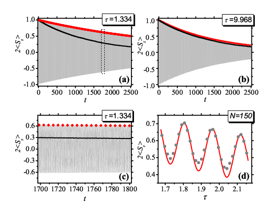
Different regimes of the rotary echo decay for a slow bath are demonstrated in Fig. 3. In agreement with our analytical results, the rotary echo envelope survives much longer than the ordinary Rabi oscillations, as long as the driving reversal period is short, . As approaches , the rotary echoes die off with virtually the same rate as the Rabi oscillations; the numerically simulated decay is in complete quantitative agreement with our analytical result (22). Note that although may look like a small number, but due to the long evolution time, the bath dynamics is important, and the rotary echo decay differs from the case of a purely static bath.
Figure 4 presents typical simulation results for a fast bath. Again, one can see that the rotary echo protocol is efficient in the short- regime. The numerical results show that Eq. (32) very accurately describes the echo amplitudes. In particular, numerical simulations in Fig. 4(d) demonstrate that performance of the rotary echo protocol, in quantitative agreement with Eq. 32, indeed depends on the value of in an oscillatory fashion for fixed , and the best protection against decoherence is provided when is chosen according to Eq. 31. Also note that , somewhat non-intuitively, corresponds to a regime of the fast bath, in spite of the fact that .
V Rotary echo protocol for realistic bath of N atoms in diamond
As mentioned above in Sec. II, the realistic bath consisting of substitutional N atom (P1 centers) in diamond has more complex structure than a single O-U field. Due to the complex internal structure of the P1 centers, where an electron spin is strongly ( MHz) coupled to a nuclear 14N spin via anisotropic hyperfine interaction, the bath of P1 centers contains six different spectral groups [11, 39, 42, 62]. Correspondingly, such a bath should be described as a sum of six O-U noise fields [42] (, with the corresponding parameters and .
Besides, the NV electron spin interacts with the nuclear spin of the NV’s own 14N atom with the hyperfine constant MHz, which has the same order of magnitude as , and has to be taken into account. The nuclear spin state, and thus the hyperfine field created by it, is static on a timescale of a single experimental run, but varies from one run to another, and therefore can be described as a static field, which randomly assumes the values (corresponding to the three states of the nuclear 14N spin ).
Below, we use the analytical results obtained above to investigate the realistic bath of P1 centers, taking into account the multiple noise fields and the on-site hyperfine coupling to the NV’s own 14N nuclear spin. We present analytical results, and compare them with the direct numerical simulations, demonstrating the quantitative agreement between analytics and numerics.
V.1 Decoherence by multiple noise fields
Because the equation of motion (5) is linear in , our theory can be generalized to include six noise fields. Introducing independent oscillator modes for each of the noise fields, , and taking to define the dimensionless quantities according to Eq. 10, we find that the evolution of the NV spin is governed by the dynamical equation similar to Eq. 11, but now with a modified pseudo-Hamiltonian:
| (33) |
where and .
It is seen that the presence of the external driving leads to mixing between different oscillator modes, so that the six oscillators are no longer independent. We can straightforwardly extend the analysis described above (single noise with large driving ) to the six-oscillator case, and readily recover Eqs. 16–18, with the simple replacement of the combination, by . Consequently, Eq. 19, with now denoting the state vector , yields correct result for the rotary echo amplitude. However, the evaluation of now becomes complicated, because now the reduced pseudo-Hamiltonian
| (34) |
involves a mixture of different oscillator modes.
We can map the sum onto a single effective oscillator coordinate , while keeping the remaining five modes, , , decoupled from the spin. This is effected by a linear transformation of the original oscillator operators via a real orthogonal matrix , such that . Introducing and , the transformed operator reads
| (35) |
where
Here replicates Eq. 18, with standing for the only oscillator mode coupled to the pseudo-spin, and is the internal pseudo-Hamiltonian of the remaining five oscillator modes. The last term in Eq. (35) is the interaction between and the remaining five modes, characterized by the strength,
| (36) |
The central spin dynamics can be studied analytically in the regime when this coupling is weak, i.e. when holds, where is the typical level spacing of the Hamiltonian . Assuming that there is no resonance between the lowest levels of and , the contribution of the interaction Hamiltonian to the eigenvalues of is of order of , and can be neglected.
Within this approximation, decouples from , and gives no contribution to the matrix element (19). In this case, the rotary echo decay is caused exclusively by the mode, whose correlation decay rate is . Hence the six O-U noise fields are essentially combined into a single effective O-U field, with the rms , and the correlation decay rate . As a result, Eq. 22 and the subsequent results of Sec. III for can be used, with replacement of by .
| # of field | 1 | 2 | 3 | 4 | 5 | 6 |
|---|---|---|---|---|---|---|
| b () | 0.83 | 1.59 | 1.63 | 1.58 | 0.8 | 1.97 |
| R () | 39 | 42 | 139 | 7 | 4 | 6 |

With the fixed values of and , as measured in recent experiments [62], the weak-coupling regime corresponds to a limited magnitude of . At the same time, in order to ensure good protection against decoherence, should not be small. The experimentally measured bath parameters correspond to and , which means that the weak-coupling regime holds for . Thus, we can expect that the analytical results above are quantitatively accurate, say for , or, in dimensional units, for an experimentally meaningful range of MHz MHz.
To gain quantitative insights, we performed numerical simulations, starting from the rotating frame Hamiltonian, , with the experimentally measured parameters of the six bath fields. In Fig. 5, the numerical results are compared with the analytical values of , obtained from Eq. (32) with . The values of are chosen according to Eq. (31) to ensure the best decoupling from the bath. Analytical and numerical results agree very well in the experimentally relevant regime of short .
For stronger driving, beyond the weak-coupling regime, six bath fields start interacting with each other. In this regime, our approximate analytical results predict faster rotary echo decay than is actually seen from the direct simulations. Thus, the analytics above can be considered as an estimate from below for the real decay curve in this regime, and therefore remains useful even for strong driving.
It is important to note that the effective values of and , which govern the rotary echo decay, are the same as those which govern the free decay, spin echo dynamics, and the response to dynamical decoupling of the NV center’s spin [39, 42, 62]. Thus, the same picture of a single effective O-U random field, with the same parameters, can describe a wide variety of the dynamical regimes for the controlled spin of a NV center.
V.2 Influence of the hyperfine coupling
In order to incorporate the on-site hyperfine coupling, the pseudo-Hamiltonian (11) should be modified in a straightforward manner, acquiring the form
| (37) |
where . Provided that , as it happens in real experiments, further analysis can be performed along the lines of Sec. III leading to the result akin to Eq. (19). Namely, for , the rotary echo amplitude is well approximated by
| (38) |
where is determined by the reduced pseudo-Hamiltonian operators,
| (39) |
Analytic form of is found in Appendix E. Because of its cumbersome form we do not present the general analytical answer here. Instead we bring the short- result,
| (40) |
This suggests that the hyperfine coupling leads to the suppression of fraction of the total signal by . With the realistic experimental numbers we have . Therefore, the fraction of the signal decays much faster than the remaining part.
Some comments on the approximation leading to the analytic form for and eventually to Eq. (40) are appropriate. The approximation is base on the assumption, . At the same time, its accuracy is guaranteed only when , where has a short-time asymptotics (23) [cf. Eq. (86) in Appendix C]. The latter condition can be violated because of a small value of or ultra-short . By considering the static limit it can be shown that the short- correction to is negative and . In contrast to the large- correction, Eq. (30), this correction does not accumulate with , and gets completely washed out for and larger. Another difference is that while Eq. (30) is due to the dynamics of the noise field, this correction is because of static hyperfine and noise fields. In order to get rid of this negative correction, one can choose to satisfy , or in dimensional units. [58] Note that the obvious conflict between this choice and the best decoupling condition Eq. (31) is insignificant, and the latter condition can be neglected. This is because the parameter domain where the correction is tangible, the large- correction Eq. (30) is negligibly small.
In Fig. 6 we compare our analytical predictions with the results of numerical simulations. Simulations are based on the rotating-frame Hamiltonian, , where takes three values, and , with equal probability. The analytical results agree well with the numerical simulations, justifying the approximations made in course of derivation. To highlight the correction, we set and , for the plots with MHz, s and MHz, s, respectively. The protocol quarter-periods for the remaining plots are chosen to satisfy the best decoupling condition Eq. 31. Divergencies between the simulated points and analytical curves for MHz, s and MHz, s are noticeable for the short total times with . This demonstrates the onset of the correction, in full agreement with the above discussion.

VI Conclusions
We considered the decay of rotary echoes for a central spin, decohered by a surrounding environmental spins, focusing on the symmetric rotary echo protocol which ensures good protection against decoherence for strong driving. We approximated the impact of the spin bath by a random time-varying magnetic field, described as Ornstein-Uhlenbeck random process (which is Markovian, Gaussian, and stationary). We obtained analytical description for different dynamical regimes, and applied our analytical results to investigating the decay of the rotary echoes for a NV center in diamond decohered by a bath of substitutional N atoms (P1 centers), which is the main decoherence source in type Ib diamonds.
Our analytical treatment is based on the mapping of the problem on the model of a spin coupled to a single bosonic mode, which has been established in Sec. III. We note here an interesting parallel with the Wiener-Hermite expansion, applied earlier in the study of the Landau-Zener transition, when crossing energy levels are subject to fluctuations due to a noisy environment. [86] This expansion appears naturally in our approach; in the present paper we did not pursue this direction, but it might be an interesting subject for further research.
Analytical form of the rotary echo amplitudes is obtained in the limit of large driving. Comparing our analytical results with direct numerical simulations, we found very good quantitative agreement. Our analysis identified two main sources of the rotary echo decay. One is the decay caused by the random field during the periods of constant driving, and this channel is most effective at not-too-long times (). The other is the decay caused by a more delicate mechanism: during each reversal of the driving, the effective quantization axis of the spin slightly changes, but these changes accumulate with time, and may become important when the total number of reversals is large (). We have also found that the latter channel is least destructive when the reversal time is commensurate with the driving period, see Eq. 31.
For sufficiently frequent reversals (small ) the symmetric rotary echo protocol ensures excellent protection of the spin. It is interesting to compare it with the protection offered by the pulse-based dynamical decoupling: for instance, for small and slow baths with , the echoes for the pulse-based decoupling decay as , while the rotary echoes decay as (here we assumed that the time between two reversals is the same as the inter-pulse delay in the Carr-Purcell-Meiboom-Gill protocol [60]). This comparison shows that the decay rate is diminished by a large factor , although achieved due to constant application of strong driving to the central spin. For realistic parameters[42], and MHz, the rotary echo decay time survives longer by a factor of about . In realistic experiments, on such time scales the decay of the NV spins would be probably dominated by other relaxation mechanisms.
It is also worth noticing that the symmetric protocol considered here, with the cycle , is more efficient than the asymmetric protocol , where the driving is switched after every time interval of . Most easily this can be seen in the limit of static bath, , where the echo decay can be found exactly. For large and , the echo amplitude of the asymmetric protocol is given by the integral
| (41) |
Obviously, the above integral is always positive and -dependent. This dependence is noticeable in experimentally relevant regime, , , where the integral takes values of order , leading to the suppression of signal. In contrast, corresponding integral for the symmetric protocol is , for arbitrary and .
Representing the real bath of P1 centers as six independent O-U random fields (corresponding to the six spectral lines of the P1 centers), we considered the decay of rotary echoes for a NV spin, also taking into account the on-site hyperfine coupling. We found that for the experimentally interesting region of large (but not too large) drivings, the six bath fields can be replaced by a single effective O-U random field. The parameters and , which describe this field and hence govern the decay of rotary echoes, are the same as the parameters which govern the free decay, spin echo dynamics, and the response to dynamical decoupling of the NV center’s spin. Thus, the same picture of a single effective O-U random field, with the same parameters, can describe a wide variety of the dynamical regimes for the controlled spin of a NV center [39, 42, 62].
Combining all results together, we identified the regimes where the symmetric rotary echo protocol most efficiently protects the NV spin. Our results may provide useful guidelines for understanding of the dynamics of a driven NV spin, and for planning future experiments. It can also be applied to a variety of other spins coupled to the dilute dipolar baths, such as donors in silicon or magnetic ions in non-magnetic host crystals. [63, 64, 65, 66]
VII Acknowledgements
We thank M. E. Raikh and L. Cywinski for interesting and useful discussions. Work at the Ames Laboratory was supported by the U.S. Department of Energy, Office of Science, Basic Energy Sciences, Division of Materials Sciences and Engineering. The Ames Laboratory is operated for the U.S. Department of Energy by Iowa State University under contract No. DE-AC02-07CH11358.
Appendix A
In this Appendix we establish the relation (16) for the single-cycle evolution operator, valid for . We begin with transforming the pseudo-Hamiltonian (11), to one that commutes with the large driving, , within a certain accuracy. This accuracy is specified by the values of and . We are going to discard the terms and , presuming , and . Hence the accuracy should extend up to . At the first step, we apply the transformation
| (42) |
where is assumed small. Neglecting the terms of order , , we write
| (43) | |||||
To cancel the term containing in , we choose the parameter . Then the last term in Eq. (43) should be kept in order to achieve the necessary accuracy, since contains a term of order of . We find:
| (44) |
To get rid of the leading inconvenient term, which does not commute with , we next apply a transformation with the operator,
| (45) |
This leads to the relation,
| (46) |
Subsequent transformations with
| (47) |
discard further inconvenient terms, up to the third order in . As a result, we get
| (48) |
where includes the above four subsequent transformations in the mixed pseudospin-oscillator space. Some comments on these transformations are in order. The first of them, , is unitary. is smaller than and invariant with respect to the sign reversal of . and contain even smaller exponents, , thus seem to be beyond our accuracy goal. At this point one should be more careful, as still contains the large term , which may amplify the effect of and . However, we will see that this is not the case and the latter operators can be safely ignored. From Eq. (15) we have
| (49) |
with and . Here we have taken into account that the -dependence of the remainder of Eq. (49) is inessential. The large terms commute with the remaining parts of , so that we can separate the corresponding exponents:
| (50) |
Therefore the matrix element (49) is equal to
| (51) |
Now consider the product, . Using the fact that is even with respect to the sign of while the rest of are odd, we write
| (52) |
where are given by Eqs. (42), (45), and (47), upon the substitution, . Explicitly, , while . Thus we see that the large parameter ends up in the arguments of sines and cosines, leaving the transformations and with exponents still suppressed as . Exactly the same applies to the other product, , and the operators, , entering this product. Because there is no longer large parameter remaining in , these transformations are negligible in Eq. (51). Therefore, all and operators inside and in Eq. (49) are negligible, too. In turn, the two properties of , namely that , and , allow us completely discard from equation (49) as well. As a result, we arrive at the relation,
| (53) |
with
| (54) |
which is a more disclosed form of Eq. (16). Obviously, the difference between and is . In addition, the norm of is less than . Hence the contribution from the -operators outside the parentheses in the matrix element Eq. (53) is at most [85] and does not accumulate with . We neglect this contribution and write:
| (55) |
Using the smallness of the exponent of , we further separate the principal part of and consider in Eq. (54) as a correction. This is done by introducing the operator
| (56) |
To the first order in , Eq. (54) reads
| (57) |
where the principal part of the single cycle time evolution operator is given by
| (58) |
whereas
| (59) |
is a perturbation. In Appendix C we demonstrate that the last term in Eq. (57) yields in fact a correction to the eigenvalue of . Therefore the rotary echo amplitudes are well described by Eq. (19), provided that . For larger , however, the contribution of is considerable. In Appendix D we calculate this contribution for larger numbers, .
Appendix B
In this Appendix we evaluate from Eq. (19), by solving the eigenvalue problem for .
The operators contain , so that we introduce the normalized eigenvectors, , . In the basis of Eq. (9) their explicit forms are:
| (60) |
Hence the state is
| (61) |
where is the ground state of the oscillator mode.
The last term of , Eq. (48), is a scalar in the subspace , decoupled from the oscillator mode. This term leads to longitudinal relaxation along the axis. Although it is the easiest to handle, throughout this Appendix we ignore it, as its contribution for is negligible. Then for we write
| (62) |
where , and with
| (63) |
From Eqs. (60)- (62) we express the matrix element as
| (64) |
To calculate the latter, we bring into the form of a single exponent. This can be done by noticing that the combinations,
| (65) |
satisfy the commutation relations of the Lie algebra, . This algebraic property allows to write in terms of the single exponent,
| (66) |
where the real positive and the complex unit vector are given in terms of the combination, , and its complex conjugate, as follows:
| (67) | |||
In the same way we represent as
| (68) |
with
| (69) | |||
| (70) | |||
| (71) |
Note that while the angle is a real number not sensitive to the sign of , the complex unit vector depends on that sign, reflecting the difference between and .
The eigenvalue problem of with a general (complex) is solved by employing the identity,
| (72) |
where and . Hence the eigenfunctions of are , where are the oscillator eigenstates (eigenfunctions of ), and the corresponding eigenvalues are equal to . In our case we have . At the same time, up to an inessential factor, acting on a state function with the squeezing operator, , results in the multiplication of its argument by . We thus get , with , and the normalized eigenfunctions,
| (73) |
where and are the Hermite polynomials. Explicitly, we have solved the eigenvalue problem,
| (74) |
On the ground of this solution we find the matrix element Eq. (64) as follows. The normalized wavefunction, , is expanded in terms of the eigenstates of by , with the coefficients,
| (75) |
After the integration, survive only coefficients with even ,
| (76) |
From this expansion and Eq. (74) we get:
| (77) |
where the last equality is due to the relation, . It is straightforward to check that Eq. (21) is simply a different form of the relation Eq. (71) for . Finally, the result Eq. (22) follows from Eq. (64), by taking real part of Eq. (77).
Appendix C
In this Appendix we analyze the perturbation , Eq. (57), and show that its contribution to the eigenvalues of is basically .
From Eq. (56) it is straightforward to check that does not have diagonal matrix elements in the eigenvector basis of . Therefore the perturbation does not have such diagonal matrix elements either. In particular, as follows from Eq. (59), the only non-zero matrix elements of are the ones between the states and , provided that ,
. This means that to the first order in there is no corrections to eigenvalues of due to , and the spectrum of is affected by only to the order of .
This proves our statement for general values of parameters. However, some complications can arise when the eigenstates and are degenerate. In the remainder of this Appendix we demonstrate that the degeneracy does not lead to any significant effect, as the resulting correction from becomes comparable with the principal part from only when both these quantities are strongly suppressed, i.e., when the central spin is completely decohered.
The above mentioned degeneracy means that and have equal eigenvalues. From the spectra of these operators found in Appendix B one can see that this is the case when
| (78) |
where is non-negative because . Once this happens, lifts the degeneracy, contributing in the eigenvalue of , and mixing the states with . More specifically, if and denote matrix elements between the degenerate states, the correct eigenvectors of are
| (79) |
instead of and , with the corresponding eigenvalues,
| (80) |
From more detailed analysis of Eq. (59) we find that the conjugate matrix elements of are the same,
| (81) |
leading to the corrected eigenvectors and eigenvalues .
Quantitatively, we can take the degeneracy in the th channel into account by modifying the term, , in the sum Eq. (77). As is orthogonal to , the degenerate channel will contribute by the amount,
| (82) |
Certainly, the only channels of interest are ones with the lowest numbers, and , or otherwise the corresponding eigenstates do not contribute appreciably. We thus consider only . From the definition it also follows that , so that we have
| (83) |
Then the contribution Eq. (82) can be cast to the form
| (84) |
so that the leading correction to Eq. (22) is given by
| (85) |
For small this correction is and thus irrelevant. For larger , on the other hand, the exponent kicks in, and the correction is suppressed exponentially, unless and . Hence we conclude that the decay of may appreciably deviate from Eq. (22) only at small .
Besides, on general grounds one should expect that the perturbative arguments fail when the level spacing of the non-perturbed operator is comparable with eigenvalues of the perturbation. This can happen when
| (86) |
We will now discuss the domain and show that the correction is of order . To treat the slow and fast baths in equal mode, we explicitly describe the boundary of the domain as
| (87) |
While for fast bath the first condition implies that the second one fulfills, for slow bath the domain boundary is defined by the second inequality, entailing the first one. To the leading order over the small parameters , , we arrive at the decomposition
| (88) | |||||
| (89) |
Here and in subsequent calculations it is important to keep operator content of the exponents, while we expand their scalar coefficients. For this reason we still keep the terms . For later convenience we introduce the parameter , though it is expressed via and . This choice descends from the fact that while for fast bath , for slow bath it can be large despite the restrictions Eq. (87). Utilizing the decomposition Eq. (88) with for and Eq. (89) for , we write the half-cycle evolution operator in the form
| (90) |
where we introduced , , and
| (91) |
First we analyze the domain of large . We express in terms of a single exponent. The three exponents at the middle of product Eq. (91) commute in the oscillator sector, so that we have a combination, with commuting and . It is easy to see that is the eigenvector of this combination, with the ”eigenvalue” . In the complementary subspace spanned over and , on the other hand, the action of the pseudospin operators are expressed via Pauli matrices as , . Exploiting the algebra of Pauli matrices we get:
| (92) |
The same as above applies to this product; the three exponents commute in the oscillator sector, so that after rotating around we get a single exponent,
| (93) |
where we have introduced the coefficients
| (94) |
which are restricted operators in the oscillator subspace: . It is now seen that terms in Eq. (90) perform a rotation around by a negligibly small angle. We disregard these terms and proceed with expressing in terms of a single exponent. The fact that we have to keep terms linear in small parameters only leads to the huge simplification, as anticipated operators in the single exponent will not contain interference terms , from different small operators. More precisely, from the perspective of the Campbell-Baker-Hausdorff formula and within the adopted accuracy, we have
| (95) |
One however has to take the precaution that in the exact combination, , higher terms can arise with large coefficients. This in turn would mean that the small expansion fails, i.e., the limit is singular. Based on the analytic forms of , , and , we do not expect such a failure of the small- expansion, and proceed with Eq. (95). We evaluate the argument of the logarithm in (95) using the symmetry Eq. (65), as in the pseudospin sector the three exponents are commutative, and find:
| (96) |
Taking into account that and are odd with respect to the sign of , while , , and are even, we also have
| (97) |
Within the given approximation, is small and should be discarded. To find the whole time evolution operator , Eq. (54), we multiply Eqs. (96) and (97):
| (98) |
We now need to express the product of the two exponents in the middle of Eq. (98) in terms of a single exponent. In this single exponent, the largest will apparently be the term, . Except for this, we have to find terms linear in , , and , and ignore the ones that contain products or higher powers of these small quantities. Particularly, if we denote by the operator of the resulting single exponent linear in , from the Campbell-Baker-Hausdorff formula we find that the very same operator emerges in a simpler situation, as
| (99) |
We evaluate this product utilizing the algebra of Pauli matrices as above, and find:
| (100) |
Evaluating the remaining small, and operators, and applying the rotation with , we get
| (101) |
Let’s now consider the exponent in Eq. (101) as the operator , perturbed with three smaller operators, , and . This unperturbed operator is diagonal in the pseudospin sector, while the last term in the square brackets does not have a diagonal in that sector. Therefore the latter term, representing correction due to , contributes in the eigenvalue of (contributions as small as or are also excluded). This statement holds down to or . When crosses over to smaller values, Eq. (101) is formally no longer valid. For small , however, can be simply found by adding up the small exponents in Eq. (90), as commutators amongst them are now suppressed at least quadratically. The result
| (102) |
nonetheless, coincides with the small- limit of (101). Here the last term corresponds to . While is the eigenvalue of Eq. (102) in the pseudospin space, owing to the last term does not contribute in the matrix element at all (recall that ). Meanwhile, the remaining two terms in Eq. (102) represent , so that in this limit the result Eq. (22) becomes even more accurate.
Appendix D
In this Appendix we calculate the correction to the matrix element, Eq. (19). Our starting point is Eq. (55), which contains all secular terms . We extend the expansion of to the second order and write:
| (103) |
where is given by Eq. (59), which we rewrite here as
| (104) |
while is found from Eq. (54) to be
| (105) |
For the matrix element Eq. (55) we have:
| (106) |
Here we introduced the operator,
| (107) |
where the sums imply , and , respectively. We first look at the limit of static bath, . It is easy to see that in this limit . Besides, in this limit can also be found; a simple calculation yields the form, , with a positive , which depends on only weakly. Therefore, for the matrix element of we have
| (108) |
where incorporates all the secular terms, accumulating with . This simple analysis suggests that the correction is suppressed for small . We thus restrict our consideration to . As we keep the short- regime, the latter condition also means a fast bath, .
To find the matrix element , we turn to the eigenstates of in the oscillator sector, i.e., the eigenstates of , denoted by and explicitly presented in Eq. (73). We notice that in this domain of parameters are very close to the oscillator states . It follows directly from Eq. (73), where we have , and close to unity, . Particularly, this fact leads to the relation, , which entails the exponential dependence Eq. (27). Utilizing this fact and Eqs. (61), (62) we write:
| (109) | |||
| (110) |
Similarly, in the domain of parameters under consideration, the eigenvectors of in the oscillator sector nearly coincide with the oscillator eigenstates. We evaluate the remaining matrix elements of and from Eqs. (104) and (105), where the exact eigenvalues of are kept, while the eigenvectors are replaced with the corresponding oscillator states. The resulting matrix element of reads:
| (111) |
where we have introduced small through . With , the last term of Eq. (111) can be neglected. Approximations made in course of this calculation, consisting in the substitution of eigenvectors of and by corresponding oscillator states, lead to the error, or . As has the same order of magnitude, we discard it from the argument of hyperbolic function. The correction to thus acquires the compact form,
| (112) |
Appendix E
In this Appendix, we evaluate the quantum mechanical average for , with given by Eq. (39), and find for .
In full analogy with Eq. (64) for , we have , where , and
| (113) |
We relate to the operator with , which was already introduced in Appendix B, cf. Eq. (63). This is done by exploiting the relation,
| (114) |
and its counterpart for , where is replaced with its complex conjugate, . We get:
| (115) |
From the commutation relations between , , and , one can infer the identity,
| (116) |
where was also introduced in Appendix B. Using the exponential form of , Eq. (68), we rewrite as
| (117) |
Next we notice the commutation relations, , where . At the same time, is a scalar, so that the first and third exponents in Eq. (117) are easily expressed via :
| (118) |
where
| (119) |
It is now straightforward to cast into the form of a single exponent from Eq. (118), using the identity, , which follows for any two operators and with the commutator, . Introducing
| (120) |
the resulting entangled form of reads:
| (121) |
The combination in rectangular brackets of the exponent Eq. (121) is equal to , so that using Eq. (115) we get:
| (122) |
From this relation, the sought expectation value, , is expressed via the one involving as
| (123) |
The action of translation on a wave function results in a shift of its argument by . Consequently, the normalized vector is expanded in terms of the eigenvectors of , Eq. (73), by
| (124) |
where are Hermite polynomials. Carrying out the integration yields:
| (125) |
This relation extends Eq. (75) to non-zero values of . The matrix element Eq. (123) is expressed in terms of the sum, . The analytic expression for the sum is possible by virtue of the relation, . We find:
| (126) |
where is factored out by using Eq. (77). To visualize this behavior, we make use of Eqs. (69)-(71) and derive the short- asymptotes,
| (127) |
We also notice that for typical values of parameters the last term in the exponent of Eq. (126) saturates with rapidly. Effectively, for relevant values of one has:
| (128) |
Thus the last term of Eq. (126) is and does not accumulate with . Neglecting this term, and using Eqs. (27), (38), we arrive at the short- form Eq. (40).
References
- [1] A. Gruber, A. Dräbenstedt, C. Tietz, L. Fleury, J. Wrachtrup, and C. von Borczyskowski, Science 276, 2012 (1997).
- [2] J. Wrachtrup and F. Jelezko, J. Phys.: Cond. Mat. 18, S807 (2006).
- [3] A. Batalov, C. Zierl, T. Gaebel, P. Neumann, I.-Y. Chan, G. Balasubramanian, P. R. Hemmer, F. Jelezko, and J. Wrachtrup, Phys. Rev. Lett. 100, 077401 (2008).
- [4] L. Robledo, L. Childress, H. Bernien, B. Hensen, P. F. A. Alkemade and R. Hanson, Nature 477, 574 (2011)
- [5] L. Childress, M. V. Gurudev Dutt, J. M. Taylor, A. S. Zibrov, F. Jelezko, J. Wrachtrup, P. R. Hemmer, and M. D. Lukin, Science 314, 281 (2006).
- [6] G. Balasubramanian, P. Neumann, D. Twitchen, M. Markham, R. Kolesov, N. Mizuoschi, J. Isoya, J. Achard, J. Beck, J. Tisler, V. Jacques, P. R. Hemmer, F. Jelezko, and J. Wrachtrup , Nat. Mater. 8, 383 (2009).
- [7] P. C. Maurer, G. Kucsko1, C. Latta, L. Jiang, N. Y. Yao, S. D. Bennett, F. Pastawski, D. Hunger, N. Chisholm, M. Markham, D. J. Twitchen, J. I. Cirac, and M. D. Lukin, Science 336, 1283 (2012).
- [8] V. V. Dobrovitski, G. D. Fuchs, A. L. Falk, C. Santori, and D. D. Awschalom, Ann. Rev. Cond. Matter 4, 23 (2013) and references therein.
- [9] F. Jelezko, T. Gaebel, I. Popa, A. Gruber, and J. Wrachtrup, Phys. Rev. Lett. 92, 076401 (2004).
- [10] G. D. Fuchs, V. V. Dobrovitski, D. M. Toyli, F. J. Heremans, and D. D. Awschalom, Science 326, 1520 (2009).
- [11] R. Hanson, V. V. Dobrovitski, A. E. Feiguin, O. Gywat, and D. D. Awschalom, Science 320, 352 (2008).
- [12] G. D. Fuchs, G. Burkard, P. V. Klimov, and D. D. Awschalom, Nat. Phys. 7, 789 (2011).
- [13] C. Santori, P. Tamarat, P. Neumann, J. Wrachtrup, D. Fattal, R. G. Beausoleil, J. Rabeau, P. Olivero, A. D. Greentree, S. Prawer, F. Jelezko, and P. Hemmer, Phys. Rev. Lett. 97, 247401 (2006).
- [14] B. B. Buckley, G. D. Fuchs, L. C. Bassett, and D. D. Awschalom, Science 330, 1212 (2010).
- [15] E. Togan, Y. Chu, A. S. Trifonov, L. Jiang, J. Maze, L. Childress, M. V. G. Dutt, A. S. Sørensen, P. R. Hemmer, A. S. Zibrov, and M. D. Lukin, Nature 466, 730 (2010).
- [16] A. Faraon, C. Santori, Z. Huang, V. M. Acosta, and R. G. Beausoleil, Phys. Rev. Lett. 109, 033604 (2012).
- [17] C. G. Yale, B. B. Buckley, D. J. Christle, G. Burkard, F. J. Heremans, L. C. Bassett, and D. D. Awschalom, Proc. Natl. Acad. Sci. 110, 7595 (2013).
- [18] P. Tamarat, T. Gaebel, J. R. Rabeau, M. Khan, A. D. Greentree, H. Wilson, L. C. L. Hollenberg, S. Prawer, P. Hemmer, F. Jelezko, and J. Wrachtrup, Phys. Rev. Lett. 97, 083002 (2006).
- [19] L. C. Bassett, F. J. Heremans, C. G. Yale, B. B. Buckley, and D. D. Awschalom, Phys. Rev. Lett. 107, 266403 (2011).
- [20] F. Dolde, H. Fedder, M. W. Doherty, T. Nöbauer, F. Rempp, G. Balasubramanian, T. Wolf, F. Reinhard, L. C. L. Hollenberg, F. Jelezko, and J. Wrachtrup, Nat. Phys. 7, 459 (2011).
- [21] T. van der Sar, Z. H. Wang, M. S. Blok, H. Bernien, T. H. Taminiau, D. M. Toyli, D. A. Lidar, D. D. Awschalom, R. Hanson, and V. V. Dobrovitski, Nature (London) 484, 82 (2012).
- [22] H. Bernien, B. Hensen, W. Pfaff, G. Koolstra, M. S. Blok, L. Robledo, T. H. Taminiau, M. Markham, D. J. Twitchen, L. Childress, and R. Hanson, Nature 497, 86 (2013).
- [23] F. Dolde, I. Jakobi, B. Naydenov, N. Zhao, S. Pezzagna, C. Trautmann, J. Meijer, P. Neumann, F. Jelezko, and J. Wrachtrup, Nat. Phys. 9, 139 (2013).
- [24] L. Childress, J. M. Taylor, A. S. Sorensen, and M. D. Lukin, Phys. Rev. Lett. 96, 070504 (2006).
- [25] P. Cappellaro, L. Jiang, J. S. Hodges, and M. D. Lukin, Phys. Rev. Lett. 102, 210502 (2009).
- [26] J. M. Taylor, P. Cappellaro, L. Childress, L. Jiang, D. Budker, P. R. Hemmer, A. Yacoby, R. Walsworth, and M. D. Lukin, Nat. Phys. 4, 810 (2008).
- [27] C. L. Degen, Appl. Phys. Lett. 92, 243111 (2008).
- [28] P. Maletinski, S. Hong, M. S. Grinolds, B. Hausmann, M. D. Lukin, R. L. Walsworth, M. Loncar, and A. Yacoby, Nature Nano. 7, 320 (2012).
- [29] N. M. Nusran, M. U. Momeen, and M. V. G. Dutt, Nature Nano. 7, 109 (2012).
- [30] L. P. McGuinness, Y. Yan, A. Stacey, D. A. Simpson, L. T. Hall, D. Maclaurin, S. Prawer, P. Mulvaney, J. Wrachtrup, F. Caruso, R. E. Scholten, and L. C. L. Hollenberg, Nature Nano. 6, 358 (2011).
- [31] T. H. Taminiau, J. J. T. Wagenaar, T. van der Sar, F. Jelezko, V. V. Dobrovitski, and R. Hanson, Phys. Rev. Lett. 109, 137602 (2012).
- [32] S. Kolkowitz, Q. P. Unterreithmeier, S. D. Bennett, and M. D. Lukin, Phys. Rev. Lett. 109, 137601 (2012).
- [33] N. Zhao, J. Honert, B. Schmid, M. Klas, J. Isoya, M. Markham, D. Twitchen, F. Jelezko, R.-B. Liu, H. Fedder, and J. Wrachtrup, Nature Nano. 7, 657 (2012).
- [34] H. J. Mamin, M. Kim, M. H. Sherwood, C. T. Rettner, K. Ohno, D. D. Awschalom, and D. Rugar, Science 339, 557 (2013).
- [35] T. Staudacher, F. Shi, S. Pezzagna, J. Meijer, J. Du, C. A. Meriles, F. Reinhard, and J. Wrachtrup, Science 339, 561 (2013).
- [36] D. M. Toyli, C. F. de Las Casas, D. J. Christle, V. V. Dobrovitski, and D. D. Awschalom, Proc. Natl. Acad. Sci. 110, 8417 (2013).
- [37] P. Neumann, I. Jakobi, F. Dolde, C. Burk, R. Reuter, G. Waldherr, J. Honert, T. Wolf, A. Brunner, and J. H. Shim, Nano Lett. 13, 2738 (2013).
- [38] G. Kucsko, P. C. Maurer, N. Y. Yao, M. Kubo, H. J. Noh, P. K. Lo, H. Park, and M. D. Lukin, Nature 500, 54 (2013).
- [39] G. de Lange, Z. H. Wang, D. Risté, V. V. Dobrovitski, and R. Hanson, Science 330, 60 (2010).
- [40] C. A. Ryan, J. S. Hodges and D.G. Cory, Phys. Rev. Lett. 105, 200402 (2010).
- [41] B. Naydenov, F. Dolde, L. T. Hall, C. Shin, H. Fedder, L. C. L. Hollenberg, F. Jelezko, and J. Wrachtrup Phys. Rev. B 83, 081201(R) (2011).
- [42] Z.-H. Wang, G. de Lange, D. Ristè, R. Hanson, and V. V. Dobrovitski, Phys. Rev. B 85, 155204 (2012).
- [43] N. Zhao, S. W. Ho, and R. B. Liu, Phys. Rev. B 85, 115303 (2012).
- [44] W. M. Witzel, M. S. Carroll, L. Cywinski, S. Das Sarma, Phys. Rev. B 86, 035452 (2012).
- [45] N. Bar-Gill, L. M. Pham, A. Jarmola, D. Budker, and R. L. Walsworth, Nat. Comm. 4, 1743 (2013).
- [46] G. de Lange, D. Risté, V. V. Dobrovitski, and R. Hanson, Phys. Rev. Lett. 106, 080802 (2011).
- [47] V. V. Dobrovitski, A. E. Feiguin, R. Hanson, and D. D. Awschalom, Phys. Rev. Lett. 102, 237601 (2009).
- [48] A. Laraoui and C. A. Meriles, Phys. Rev. B 84, 161403 (2011).
- [49] M. Hirose, C. D. Aiello, and P. Cappellaro, Phys. Rev. A 86, 062320 (2012).
- [50] A. Bermudez, F. Jelezko, M. B. Plenio, and A. Retzker, Phys. Rev. Lett. 107, 150503 (2011).
- [51] M. Loretz, T. Rosskopf, and C. L. Degen, Phys. Rev. Lett. 110, 017602 (2013).
- [52] P. Facchi, D. A. Lidar, and S. Pascazio, Phys. Rev. A 69, 032314 (2004).
- [53] J. Cai, B. Naydenov, R. Pfeiffer, L. P. McGuinness, K. D. Jahnke, F. Jelezko, M. B. Plenio, and A. Retzker, New J. Phys. 14, 113023 (2012).
- [54] X. Xu, Z. Wang, C. Duan, P. Huang, P. Wang, Y. Wang, N. Xu, X. Kong, F. Shi, X. Rong, and J. Du, Phys. Rev. Lett. 109, 070502 (2012).
- [55] J. Cai, F. Jelezko, M. B. Plenio, and A. Retzker, New J. Phys. 15, 013020 (2013).
- [56] C. Belthangady, N. Bar-Gill, L. M. Pham, K. Arai, D. Le Sage, P. Cappellaro, and R. L. Walsworth, Phys. Rev. Lett. 110, 157601 (2013).
- [57] P. London, J. Scheuer, J.-M. Cai, I. Schwarz, A. Retzker, M. B. Plenio, M. Katagiri, T. Teraji, S. Koizumi, J. Isoya, R. Fischer, L. P. McGuinness, B. Naydenov, and F. Jelezko, Phys. Rev. Lett. 111, 067601 (2013).
- [58] C. D. Aiello, M. Hirose, and P. Cappellaro, Nat. Comm. 4, 1419 (2013).
- [59] I. Solomon, Phys. Rev. Lett. 2, 301 (1959).
- [60] C. P. Slichter, Principles of Magnetic Resonance (Springer, Berlin, New York, 1990).
- [61] N. Bar-Gill, L. Pham, C. Belthangady, D. L. Sage, P. Cappellaro, J. Maze, M. Lukin, A. Yacoby, and R. Walsworth, Nat. Commun. 3, 858 (2012).
- [62] G. de Lange, T. van der Sar, M. S. Blok, Z.-H. Wang, V. V. Dobrovitski, and R. Hanson, Scientific Reports 2, 382 (2012).
- [63] J. J. Pla, K. Y. Tan, J. P. Dehollain, W. H. Lim, J. J. L. Morton, D. N. Jamieson, A. S. Dzurak, and A. Morello, Nature 489, 541 (2012).
- [64] J. J. L. Morton, D. R. McCamey, M. A. Eriksson, and S. A. Lyon, Nature 479, 345 (2011).
- [65] A. Morello, J. J. Pla, F. A. Zwanenburg, K. W. Chan, K. Y. Tan, H. Huebl, M. Möttönen, C. D. Nugroho, C. Yang, J. A. van Donkelaar, A. D. C. Alves, D. N. Jamieson, C. C. Escott, L. C. L. Hollenberg, R. G. Clark, and A. S. Dzurak, Nature 467, 687 (2010).
- [66] S. Bertaina, S. Gambarelli, T. Mitra, B. Tsukerblat, A. Müller, and B. Barbara,, Nature 453, 203 (2008).
- [67] B. Smeltzer, J. McIntyre, and L. Childress, Phys. Rev. A 80, 050302(R) (2009).
- [68] S. Felton, A. M. Edmonds, M. E. Newton, P. M. Martineau, D. Fisher, D. J. Twitchen, and J. M. Baker, Phys. Rev. B 79, 075203 (2009).
- [69] J. H. N. Loubser and J. A. van Wyk, Rep. Prog. Phys. 41, 1201 (1978).
- [70] P. W. Anderson and P. R. Weiss, Rev. Mod. Phys. 25, 269 (1953).
- [71] P. W. Anderson, J. Phys. Soc. Jpn. 9, 316 (1954).
- [72] R. Kubo, J. Phys. Soc. Jpn. 9, 935 (1954).
- [73] J. R. Klauder and P. W. Anderson, Phys. Rev. 125, 912 (1962).
- [74] V. V. Dobrovitski, A. E. Feiguin, D. D. Awschalom, and R. Hanson, Phys. Rev. B 77, 245212 (2008).
- [75] W. A. Coish and D. Loss, Phys. Rev. B 70, 195340 (2004).
- [76] W. M. Witzel, R. de Sousa, and S. Das Sarma, Phys. Rev. B 72, 161306(R) (2005).
- [77] S. K. Saikin, W. Yao, and L. J. Sham, Phys. Rev. B 75, 125314 (2007).
- [78] R.-B. Liu, W. Yao, and L. J. Sham, New J. Phys. 9, 226 (2007).
- [79] J. R. Maze, J. M. Taylor, and M. D. Lukin, Phys. Rev. B 78, 094303 (2008).
- [80] L. Cywinski, W. M. Witzel, and S. Das Sarma, Phys. Rev. B 79, 245314 (2009).
- [81] N. van Kampen, Stochastic Processes in Physics and Chemistry (North-Holland, Amsterdam, 1981).
- [82] E. Geva, R. Kosloff, and J. L. Skinner, J. Chem. Phys. 102, 8541 (1995).
- [83] C. Cohen-Tannoudji and S. Reynaud, J. Phys. B 10, 365 (1977).
- [84] R. Kubo, J. Math. Phys. 4, 174 (1963).
- [85] A detailed analysis shows that this contribution is .
- [86] Y. Kayanuma, J. Phys. Soc. Jpn. 53, 108 (1984); ibid. 54, 2037 (1985).