QCD sum rules on the complex Borel plane
Abstract
Borel transformed QCD sum rules conventionally use a real valued parameter (the Borel mass) for specifying the exponential weight over which hadronic spectral functions are averaged. In this paper, it is shown that the Borel mass can be generalized to have complex values and that new classes of sum rules can be derived from the resulting averages over the spectral functions. The real and imaginary parts of these novel sum rules turn out to have damped oscillating kernels and potentially contain a larger amount of information on the hadronic spectrum than the real valued QCD sum rules. As a first practical test, we have formulated the complex Borel sum rules for the meson channel and have analyzed them using the maximum entropy method, by which we can extract the most probable spectral function from the sum rules without strong assumptions on its functional form. As a result, it is demonstrated that, compared to earlier studies, the complex valued sum rules allow us to extract the spectral function with a significantly improved resolution and thus to study more detailed structures of the hadronic spectrum than previously possible.
PTEP-subject
D32, B671 Introduction
The spectral function of hadrons is one of the main targets in studies of low energy QCD. At low energy, non-perturbative approaches are inevitable as the coupling constant is large and the QCD vacuum has non-trivial quark and gluon condensates. In order to take into account effects of these vacuum condensates, QCD sum rules [1, 2, 3] have been extensively used to explore hadron spectra.
QCD sum rules utilize the operator product expansion (OPE) for evaluating correlation functions, which is valid in the deep Euclidean four-momentum region. A dispersion relation based on analyticity of the correlation function on the other hand yields a relation between an integral over the spectral function and the vacuum condensates. Inverting the integral relation and extracting the spectral function thus is the central issue of QCD sum rule analyses. In conventional approaches, the spectral function is most often parametrized using a “pole + continuum” functional form, whose parameters are determined to satisfy the sum rule. This technique is, however, not always applicable because in reality the spectral functions are not restricted to a particular shape.
Recently, a new method was proposed that directly provides the spectral function without assuming a functional shape [4]. It utilizes the maximum entropy method (MEM), which generally helps to determine the most probable spectral function from an integral relation [5]. Thus, the obtained spectral function is chosen from infinitely many functional forms, while the conventional approach only gives the best fitted “pole + continuum” type function. So far, this novel method has been applied to the -meson [4] and nucleon [6, 7] channels in vacuum and to charmonium [8] and bottomonium [9] channels at finite temperature. It has, however, not yet shown its full strength, giving only the ground state peak structure, while usually neither reproducing excitation nor continuum spectra. We believe that this is not a consequence of the limitation of MEM, but rather due to the limited information provided by the conventional QCD sum rules.
In this paper, we propose to extend the QCD sum rules to the complex plane of the squared-momentum, , by which we are able to extract more information on the spectral function.11 1 Extension of QCD to the complex plane has been proposed earlier by Ioffe and Zyablyuk [10]. As the sum rules are based on the analytic continuation of the correlation function on the plane, they can be naturally generalized to the complex plane. As a result, it is found that after using the Borel transform to enhance the convergence of the OPE, the Borel sum rule is valid also for the complex Borel parameter.
Applying the MEM to the newly constructed sum rules, we study the spectral function of the vector meson composed of the strange quark (), i.e. the spectral function in the meson channel. Our results show that the new sum rule improves the reproducibility of the spectral function compared to the conventional Borel sum rules, in particular in the large momentum region.
The paper is organized as follows. In Sec.2, we explain the central idea of our novel complex Borel plane sum rules, demonstrate in detail how the sum rules are constructed and discuss their properties. After all, it will be shown that our formulation can be considered to be just a simple generalization of conventional Borel sum rules to complex Borel mass values. Next, we briefly introduce MEM and define the likelihood function for the complex Borel plane sum rules to apply MEM to them in Sec. 3. In Sec. 4 the results of the analyses are outlined. Here, we will not only show the results of the complex Borel plane sum rules but also the ones of the original Borel sum rules for comparison. Summary and conclusions are given in Sec. 5.
2 Complex Borel sum rules
In this section, we formulate the complex Borel sum rules (CBSR). The general procedure is the same as that used for deriving the conventional QCD sum rules with real variables (RBSR).
2.1 Dispersion relation on the complex plane
The basic idea of the CBSR is to consider the squared four-momentum as a complex parameter when deriving the sum rules. The validity of this generalization is guaranteed by the dispersion relation.
The elementary ingredients of the derivation, Cauchy’s residue theorem and the analyticity of the correlator, do not restrict to real numbers but rather allow it to have any value on the complex plane except the region around the positive real axis (see Fig. 1). In other words, for the correlator , Cauchy’s residue theorem and analyticity guarantee
| (1) |
for any complex . Here, is a positive integer, chosen to be large enough for the integral to converge. The detailed definition of the depends on the specific channel. In the case of the vector channel, which will be studied in this paper, can be defined as shown in Eq.(21). Following the same steps used when deriving the conventional sum rules, we obtain the following dispersion relation (see Appendix A for details):
| (2) |
where (for a real and an infinitesimal ()) is the spectral function. Although this looks just like the conventional diversion relation, it potentially contains novel kinds of sum rules for the spectral function, extracted from both its real and imaginary parts. Our strategy is employing Eq.(2) as a starting point for deriving the actual sum rules.

2.2 Analytic continuation of the OPE
In QCD sum rules, it is common to replace the left hand side of Eq.(2) by its respective OPE, which is valid in the deep Euclidean region, i.e. large real . Extending this to the complex plane, we consider the OPE for the complex variable . In practice, the OPE must be truncated at a certain operator dimension and one can only hope that it converges at sufficiently large . In the region where the OPE is convergent, the left hand side of Eq.(2) can be extended to the complex argument as , which is the analytically continued function of . It is important to note that depends on only through the Wilson coefficients and therefore has the same vacuum expectation values of the local operators. After all, we obtain the complex sum rules as,
| (3) |
2.3 Borel transformation
The unknown polynomial in Eq.(3) can be removed by the Borel transform, defined by
| (4) |
where is a real variable.
By substituting , where is defined as shown in Fig. 1, Eq.(3) can be considered as a relation depending on and . As polynomials in z are linear combinations of , differentiating Eq.(3) infinite times by eliminates them. It is hence understood that is suitable for our present purposes. On the right hand side of Eq.(3), the integral term is transformed as
| (5) |
The integral kernel is transformed into an exponential function if the limit can be interchanged with the integral over . At first sight, this seems to be a trivially allowed manipulation, but a careful inspection, in fact, shows that it is not necessarily correct. Relying on a theorem (which is similar to Lebesgue’s “dominated convergence theorem”), it is possible to show that the two operations indeed can be interchanged for . An explicit proof of this statement is given in Appendix B. On the other hand, for , one sees that the limit and the integral over s are not interchangeable. This is so because if one could interchange the limit with the integral, the ensuing integrand would diverge exponentially at large , which is apparently inconsistent with the left hand side, which remains finite for , as we will see in the discussion given below. We thus conclude that only for , the Borel transform leads to the following result:
| (6) |
Note that this region includes (), which gives the RBSR.
Next, let us discuss the Borel transformation of the left hand side of Eq.(3). As above, we substitute into the given analytically continued OPE expression and then apply . Doing this, we obtain
| (7) |
for which detailed derivations are given in Appendix C. Here let us compare these results with the following pre-existing formulae for the corresponding real functions:
| (8) |
These all suggest that the Borel transformation of the analytically continued of OPE equals that of the original OPE with a complex valued Borel mass. We can thus set
| (9) |
where is defined as .
Finally, we obtain
| (10) |
where . This form of the complex plane QCD sum rule is nothing but the well known real valued Borel sum rule, in which the real Borel mass is replaced by its complex analogue, . Therefore, the complex Borel plane sum rules is found to be a simple generalization of the ordinary Borel sum rules to the complex Borel mass plane and of course includes the latter at .
2.4 Properties of the CBSR
Although the CBSR of Eq.(10) looks similar to its real counterpart, its content is quite different. Since Eq.(10) is complex valued, it simultaneously gives two sum rules which can be obtained from its real and imaginary part. Specifically, we have
| (11) |
where and are defined as
| (12) |
| (13) |
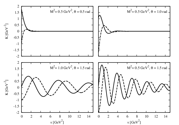
Both and are damped oscillating functions of , as shown in Fig. 2 for several combinations of and . As can be observed in these plots, the oscillations have various frequencies, phases and damping factors depending on the values of and . We can hence expect that, compared with the RBSR, the sum rules with these kernels have the potential to resolve finer structures of the spectral function.
As a further point, let us note here that the sum rules with complex Borel masses and their complex conjugates are not independent. Looking at the explicit form of the kernels, it is clear that the right hand sides of the sum rules with complex conjugated Borel masses satisfy
| (14) |
In turn, the left hand side satisfies, according to the Schwarz reflection principle,
| (15) |
Therefore the complex Borel sum rules are in essence identical to their complex conjugated counterparts.
2.5 Effective domain in complex Borel space
It is important to specify the region on the complex Borel plane, in which the CBSR of Eq.(10) (or Eq.(11)) can be effectively used for the analysis of the spectral function. Firstly, the CBSR does not work for , as we have explained in section 2.3. Secondly, the region with gives sum rules with the same content as those with positive imaginary part of . Thirdly, we have to make sure to exclude the region, where the OPE might not be a valid approximation. To this end, we use the condition employed in standard QCD sum rule analyses, namely, we demand that the highest order OPE term is smaller than a critical ratio of the whole OPE expression. We thus impose
| (16) |
which is used in the RBSR analyses with a typical value of . For the present work, we will employ the same value. The only difference to the RBSR is that we here take ratios of moduli of complex valued functions instead of real ones. Eq.(16) produces a closed curve in the complex Borel mass plane in whose inner region the sum rules can not be used.
With all these restrictions, the effective domain for the sum rule lies in the first quadrant of the imaginary plane with an excluded small region, as shown schematically in Fig. 3.
3 The maximum entropy method
Advantages of the CBSR can be most efficiently exploited with the help of the maximum entropy method (MEM). This method enables us to determine the spectral function from the sum rules without assuming a specific functional form such as the popular “pole + continuum” ansatz. Therefore, the more detailed the available information from the OPE is, the more realistic and accurate the spectral function obtained by MEM will be. Conversely, without enough physical information, the extracted spectral function will depend strongly on the “default model”, which is an input of the MEM analysis, as will be explained below. In this sense, the CBSR is very useful for the MEM analysis as it provides more physical information thanks to the rich structure of its kernels. In the next few paragraphs, we shall briefly explain the essence of MEM and point out some issues specific to the analysis presented in this paper.
MEM will lead us to the spectral function that maximizes
| (17) |
where stands for the Shannon-Jaynes entropy, defined by
| (18) |
Here, is some positive definite function called default model. (Note that we change the variable from to in the following.) ensures the positive definiteness of the spectral function and takes the maximum value at .
is the likelihood function, which incorporates physical information provided by the sum rule. In the case of the real valued Borel sum rules, it is expressed as
| (19) |
where the subscript () specifies the discretized Borel mass and is the error of the OPE data . The error is determined from the uncertainty of the vacuum condensates. The factor , appearing in the integrand of Eq.(19) is a result of the variable change from to .
The parameter is a positive real number on which the spectral function maximizing depends. The range of this parameter is determined by MEM and we take a weighted average of the obtained spectral functions over to get the final solution. For the details of this procedure, we refer the interested reader to [4].
In the application of MEM to the complex Borel plane sum rules, some modification in the likelihood function is necessary. As one complex Borel mass gives two sum rules, the real and imaginary parts, the likelihood function can be expressed as the sum of them as
| (20) |

The subscripts here specify discretized the complex Borel mass in the (2-dimensional) complex plane, and is the total number of the chosen Borel masses. The variances and are the ambiguities of the real and imaginary parts of .
The discretized Borel masses are chosen in the domain shown in Fig. 3, according to the previous discussion. The lower boundary of is determined to satisfy Eq.(16) for each independently. For the upper boundary, , we do not have a definite restriction and in principle may choose it freely. We will show dependences on different choices of in the specific example given in the next section.
4 Analyses of OPE data
In this section, the CBSR is applied to the analysis of the spectral function for the meson channel as a first test of the validity of our method. We compare the results with those of the RBSR.
4.1 The CBSR for the meson
We consider the sum rule for the vector meson composed of and , where is the strange quark. The interpolating field operator is , which is supposed to create the (1020) meson from the vacuum.
The correlation function
| (21) |
describes the spectrum of the meson and its excited states.
The OPE of the function has been obtained [2] as follows:
| (22) |
Note that in writing down the above result, we have assumed the vacuum saturation approximation for the dimension 6 four-quark condensate term and have parametrized the possible violation of this approximation by the parameter . Replacing with in Eq.(22) and performing the Borel transformation, we can easily derive the OPE for the CBSR:
| (23) |
where . As we mentioned in Sec.2, this form is equal to that of the real valued Borel sum rule, the Borel mass being simply replaced by the complex Borel mass. When we use the polar form for , the respective real and imaginary parts can be explicitly given as follows:
| (24) |
The values and uncertainties of the quark mass, strong coupling constant and and vacuum condensates appearing in the OPE used in our analysis are given in Table 1.
We choose in the condition (16) for the domain of valid complex Borel mass. It is then restricted outside the region specified in Fig. 4.
| [11] | ||
|---|---|---|
| [12] | ||
| [3] | ||
| [13] | ||
| [14] | ||
| [15] |

4.2 Analysis results with a single default model and value
In our MEM analysis, we have some freedom to choose the default model and the outer circle radius . A reasonable choice for should reflect our prior knowledge on the spectral function, because it gives its most probable form when no constraints from the sum rules are available. A suitable choice for its form is thus, as has been already discussed in [4], a function which tends to zero at low energy and approaches the perturbative high energy limit for large . A parametrization which has these properties and smoothly interpolates between the low and high energy limit, is given as
| (25) |
Note that in Eq.(24) is dimensionless in this case and is supposed to go to the asymptotic value, at high energy. For a first trial, we will use and in the analysis of this subsection and later examine the effects of other default models. As for , it should generally not be too large because for large , the damping factor of the kernels becomes weak, which means that the integrals over the spectral function in Eq.(24) will have large contributions from the continuum. should on the other hand not be taken too small to allow a sufficiently large interval above the prohibited region shown in Fig. 4. As a parameter satisfying these conditions, we choose and will later investigate the effects of different choices for this value. For comparison, we have also analyzed the RBSR of the meson channel with MEM, as it was done for the meson in [4]. The Borel mass for this analysis was taken as , which corresponds to the real axis of the area shown in Fig. 4.

The obtained results are shown in Fig. 5. Three peaks are generated in the analysis of the CBSR. The estimated errors on the MEM results are shown by the three horizontal limes at each peak. Among the three peaks, the first and second peak are statistically significant and can therefore presumably be considered to represent physical resonances. Further discussions on this point will follow in the next subsections. The third peak is on the other hand not statistically significant and hence no conclusions on its physical existence can be drawn. The positions of the first two peaks are given in Table 2, where it is observed that the peak positions agree quite well with the respective experimental values. Comparing this with the result of the RBSR on the right plot of Fig. 5, it is seen that for the latter case, only one relatively broad peak is extracted, which can be considered to be a smeared version of the first two peaks obtained from the CBSR. This is a reasonable result, as the CBSR contains more detailed information on the spectral function and thus allow for a better resolution of its MEM extraction.
| CBSR | RBSR | Experiment | |
|---|---|---|---|
| 1st peak [GeV] | 0.94 | 1.15 | 1.02 |
| 2nd peak [GeV] | 1.74 | 1.68 |
4.3 Analysis results with various choices of the default model and
To get an idea on the systematic uncertainties of our results, it is important to study the dependence of the generated spectral functions on the default model and the used value of . We will for this purpose not only use default models of the form given in Eq.(25), but also another version which contains no information on the asymptotic behavior of the spectrum at high energy. The most simple form of such a default model would be just a constant, however, much smaller than the asymptotic value, . For this reason, the following function is chosen as an alternative default model:
| (26) |
For , we take , , , and (all in units of ) to investigate the effect of a larger choice for this parameter. We have totally carried out ten different analyses for both the CBSR and RBSR, using two types of default models ( or ) and the above-mentioned five values of . The corresponding results are shown in Fig.6 and Fig.7, respectively.


Let us firstly examine the high energy region of the obtained spectral functions. Looking at the results with on the right side of Fig. 6, it is clear that for larger , the spectral functions approach the perturbative high energy limit at large values. This shows that the continuum can be reproduced by the CBSR irrespective of the chosen default model. In contrast, it is found that the reproduction of the continuum is much worse for the RBSR. As can be observed on the right side of Fig.7, MEM tries to reproduce some sort of continuum, but can only generate a strongly oscillating function with a large artificial peak somewhat above . Although the continuum is reproduced for the results with on the left side of Fig. 7, this behavior is simply a consequence of the default model used in this specific case.
Next, we focus our attention on the low energy parts of the spectrum. For the lowest peak, which corresponds to the meson ground state, the obtained positions and strengths do not much depend on the choice of or on the value of , which means that the CBSR are sensitive to this state and that the MEM can extract its properties with only small systematic uncertainties. The situation is again less clear for the RBSR results of Fig. 7, as here, even the first peak is statistically significant only for .
In the CBSR spectra of Fig. 6, it is furthermore seen that a statistically significant second peak is found for values up to . This peak however broadens and slightly moves its position as we go to larger values of . It moreover looses its statistical significance for and becomes a part of the small oscillations that appear at the edge of the continuum for the largest few values of . The properties of the second peak therefore to some degree depend on and it is not completely clear whether this peak is of physical origin or merely an artifact of the MEM analysis. We will further discuss this question in the the mock data analysis of the next subsection.
4.4 Test analysis results by using the mock spectral function
For better understanding what parts of the spectral function can be reliably studied with our method and what sort of artificial structures might appear in the MEM results, we have carried out a test analysis using the mock data generated from some specific input spectral function. Based on the results of this analysis, we will investigate whether the second peak found Figs. 5 and 6 is physical or just an MEM artifact and will further discuss the different reproducibilities of the CBSR and RBSR analyses. For the input mock spectral function of the -meson channel, we employ a relativistic Breit-Wigner peak and a smooth function describing the transition to the asymptotic value at high energies [16],
| (27) |
which has been renormalized so that the asymptotic behavior of the spectral function at high energy is consistent with Eq.(22), the OPE used in this paper. For the parameters appearing in Eq.(27), we use the following values:
| (28) |
The mock data are then numerically generated as shown below for the CBSR case:
| (29) |
In the actual MEM analysis, we have treated like OPE data, meaning that we use the the same errors and Borel mass ranges which were used in the OPE data analyses of the previous sections. Specifically, we have analyzed two cases. In the first case, we have taken and used of Eq.(25) for the default model. The respective results are shown in Fig. 8, which should be compared to Fig. 5, where the OPE data have been analyzed under exactly the same conditions. For the second case, we have used with the default model of Eq.(26), the result being shown in Fig. 9. This case corresponds to the top right plots of Figs. 6 and 7 for the OPE data analyses.


Firstly, let us investigate the mock data analysis results of the first case with . Looking at the left plot of Fig.8, it is found that for the CBSR an artificial second peak can be generated by the MEM analysis even if such a peak is not present in the original spectral function. This phenomenon can be thought of as a result of the MEM trying to reproduce the continuum, but not having enough information due to the small value of . The extracted spectral function therefore eventually approaches the default model, leading to an artificial peak. In contrast to the OPE data analysis result of Fig. 5, this peak is however not statistically significant. Also the strengths of the peaks are different: while the second peak obtained from the OPE data clearly rises above the continuum, the respective mock data peak does not. These findings show, that while it is possible that small artificial bumps or peaks can be produced by the MEM analysis, these will not be as large as the second peak seen in Fig.5. We hence can conclude that this peak is likely to reflect the properties of a physical state, the first excited state of the meson. As a further point, comparing both plots of Fig. 8, it is observed that CBSR reproduces the position of the first peak with much better precision than the RBSR. Furthermore, considering the width of the lowest peak, it is seen that CBSR shows some improvement compared to the RBSR, but is nevertheless not able to reproduce the very narrow physical width of the meson.
Next, we examine the results for . From Fig. 9, we can confirm that at large energy CBSR is able to reproduce the continuum without relying on the default model. This is not the case for the RBSR, which instead of a constant behavior produces large oscillations. On the other hand, we found that at the lower edge of the continuum, the CBSR generates artificial oscillations, which are damped out toward higher energies. It is hence understood that the periodic peaks found in the OPE data analysis above the ground state peak for large values of (see Fig. 6) are mainly MEM artifacts. Even though the spectral functions obtained from the OPE data show a somewhat stronger second peak, which can probably be explained by the existence of a physical state in that region, this difference is too small to allow any definitive conclusions. To recapitulate, for large values of , the sum rules are dominated by the continuum (which is thus well reproduced) and contains relatively less information on the low energy part of the spectrum. For obtaining information on the possible existence of excited states, one therefore needs to choose small enough values.
5 Summary and conclusion
We have in this study constructed the complex Borel plane QCD sum rules (CBSR) and have applied it to the meson channel as a first test of its validity and usefulness. We have explicitly demonstrated that the CBSR can be obtained by simply replacing the Borel mass of the real Borel QCD sum rules (RBSR) with a complex parameter . Since the Borel mass can thus take values on the complex plane and not only on the real axis, the CBSR allows us to extract more information on the spectral function than it was previously possible. To check whether the CBSR works in practice and to examine the quality of the information provided by the sum rules, we have studied the meson channel with the help of MEM. The main results of this investigation are as follows:
- •
The MEM analysis generates a clear and statistically significant lowest peak, which corresponds to the physical state. Its position is found to be only weakly dependent on the inputs of the MEM analysis, such as the default model or .
- •
A second peak, which may correspond to the first excited state of the meson channel, also appears in the obtained spectral function. This peak is, however, only statistically significant when OPE data close to the origin of the complex Borel mass plane are analyzed (i.e. when a rather low value is used). Making larger, it is found to mix with artificially generated peaks which have no physical significance and change its position to larger energy region. Hence, we presently can not make conclusive statements on the mass of the excited state since it depends on the value of . Nevertheless, the fact that the peak is statistically significant at least for low and the results of the examination using a mock spectral function is indicative of the existence of the excited state and warrants further studies once the OPE is known with better precision.
- •
Besides the lowest two peaks, we have shown that the CBSR is capable of reproducing the continuum at high energy. Specifically, as long as is chosen to be sufficiently large, the MEM analysis generates the correct high energy limit of the spectral function even if the default model has a different limiting value.
The CBSR hence appears to be a useful tool for analyzing hadronic spectral functions, which is superior to the conventional RBSR. It is important to note here that only by using MEM, we can exploit the full power of the CBSR, as MEM in principle allows the spectral function to have any specific (positive definite) form.
Acknowledgment
This work was partially supported by KAKENHI under Contract Nos.24540294 and 25247036. We would like to express our sincere gratitude to Dr. Kiyoshi Sasaki for helping us with the numerical calculations. K.O. gratefully acknowledges the support by the Japan Society for the Promotion of Science for Young Scientists (Contract No.25.6520).
Appendix A Derivation of dispersion relation
To confirm that the QCD sum rules can be formulated by complex parameters, we in this appendix derive the dispersion relation in detail. Using the analyticity of the correlator on the imaginary plane (excluding of course the region of positive real ), we can apply Cauchy’s residue theorem and obtain the following equation:
| (30) |
The contour is given in Fig.10 and z refers to complex . Firstly, the contour C is divided into as shown in Fig.10 and is supposed to be sufficiently large (but finite) so that the integral along converges to zero when taking the limit and :
| (31) |
Next, the contributions of the other contour sections are considered. By using the equation:
| (32) |
the integrals along and can be divided into terms containing only polynomials in z and terms with other analytical structures:
| (33) |
For treating the integral along the small half circle , we again use Eq.(32) to obtain
| (34) |
Note that we have assumed here that ®(s) does not have a singularity at . Adding the various contributions, we finally arrive at the desired dispersion relation:
| (35) |
The important point here is that the above equation has been derived without restricting z to real numbers. It also should be mentioned that although we have chosen the contour not to include the origin, we as well could have taken the origin to lie inside the contour. In that case, would have to be added to Eq.(30). The final result, however, does not change its form since this additional term is just another polynomial in and is thus consistent with Eq.(35).

Appendix B Proof of the interchangeability of the Borel transformation interchange with the integral over
In this appendix, we will prove that for it is possible to interchange the Borel transformation with the integral over in Eq. (5). For doing this, we rely on the following theorem [17]:
Theorem 1.
The sequence of continuous functions is defined in . It is assumed that the limit exists and that it is continuous in . Furthermore, a function which satisfies the following conditions is assumed to exist:
- •
for all and
- •
When these conditions hold, the limit of taking to infinity can be interchanged with the integral over as shown below.
| (36) |
In order to apply this theorem to the problem at hand, we use the last line of Eq.(5) and rewrite it as follows:
| (37) |
with
| (38) |
To be able to interchange the Borel transformation with the integral therefore would mean that
| (39) |
hold. Both relations can be proven for , for which one has to show that the assumptions needed for the above theorem are satisfied. For definiteness, we here only derive the first relation and note that the second one can be treated analogously. Firstly, it is clear that the limit exists and is continuous. This limit is given in Eq.(12). Next, the absolute value of the real part of can be estimated as follows:
| (40) |
As for is a monotonously decreasing function of , we obtain
| (41) |
where is a natural number. It should be kept in mind here that this inequality is only valid for . We can take to be finite so that
| (42) |
because the behavior of in the high energy region is supposed to be polynomial. Redefining by taking (which does not matter since we are intereted in the limit ), we can write
| (43) |
Identifying with the function of the theorem, the proof is complete. As mentioned above, the proof of the second equation in Eq.(39) can be done in the same way. We have hence proven that one can interchange the Borel transformation with the integral over for .
Appendix C Borel transformation on the complex plane
In this appendix, we derive the Borel transformations of the complex functions given in section 2.3, i.e.
| (44) | |||||
| (45) | |||||
| (46) | |||||
| (47) |
Although it is possible to derive them following the definition of , we for simplicitly utilize the following formulae for the Borel transformation of real functions ().
| (48) | |||||
| (49) | |||||
| (50) | |||||
| (51) |
which are consistent with Eq.(8), once is replaced with . The strategy is to separate the phase of by substituting , after which the calculations are straightforward. The first relations is easily derived,
| (52) |
while the second one is obtained as
| (53) |
The third and fourth equations are derived in a similar way:
| (54) |
| (55) |
References
- [1] M. A. Shifman, A. Vainshtein, and V. I. Zakharov, Nucl. Phys. B147, 385 (1979).
- [2] M. A. Shifman, A. Vainshtein, and V. I. Zakharov, Nucl. Phys. B147, 448 (1979).
- [3] L. Reinders, H. Rubinstein, and S. Yazaki, Phys. Rept. 127, 1 (1985).
- [4] P. Gubler and M. Oka, Prog. Theor. Phys. 124, 995 (2010).
- [5] M. Asakawa, T. Hatsuda, and Y. Nakahara, Prog. Part. Nucl. Phys. 46, 459 (2001).
- [6] K. Ohtani, P. Gubler, and M. Oka, Eur. Phys. J. A 47, 114 (2011).
- [7] K. Ohtani, P. Gubler, and M. Oka, Phys. Rev. D 87, 034027 (2013).
- [8] P. Gubler, K. Morita, and M. Oka, Phys. Rev. Lett. 107, 092003 (2011).
- [9] K. Suzuki, P. Gubler, K. Morita, and M. Oka, Nucl. Phys. A897 (2013).
- [10] B. L.Ioffe and K. N. Zyablyuk, Nucl. Phys A687, 437 (2001).
- [11] S. Borsanyi et al., Phys.Rev. D 88, 014513 (2013).
- [12] P. Colangelo and A. Khodjamirian, At the Frontier of Particle Physics/ Handbook of QCD 3, 1495 (2000).
- [13] Particle Data Group, J. Beringer et al., Phys. Rev. D 86, 010001 (2012).
- [14] D. B. Leinweber, Ann. Phys. 254, 328 (1997).
- [15] S. Bethke, Nucl. Phys. Proc. Suppl. 234, 229 (2013).
- [16] E. V. Shuryak, Rev. Mod. Phys. 65, 1 (1993).
- [17] K. Kodaira, An Introduction to Calculus (Kaiseki Nyumon I) (Iwanami-Shoten, 2003).