Spectral Sparse Representation for Clustering: Evolved from PCA, K-means, Laplacian Eigenmap, and Ratio Cut
Abstract
Dimensionality reduction, cluster analysis, and sparse representation are basic components in machine learning. However, their relationships have not yet been fully investigated. In this paper, we find that the spectral graph theory underlies a series of these elementary methods and can unify them into a complete framework. The methods include PCA, K-means, Laplacian eigenmap (LE), ratio cut (Rcut), and a new sparse representation method developed by us, called spectral sparse representation (SSR). Further, extended relations to conventional over-complete sparse representations (e.g., method of optimal directions, KSVD), manifold learning (e.g., kernel PCA, multidimensional scaling, Isomap, locally linear embedding), and subspace clustering (e.g., sparse subspace clustering, low-rank representation) are incorporated. We show that, under an ideal condition from the spectral graph theory, PCA, K-means, LE, and Rcut are unified together. And when the condition is relaxed, the unification evolves to SSR, which lies in the intermediate between PCA/LE and K-mean/Rcut. An efficient algorithm, NSCrt, is developed to solve the sparse codes of SSR. SSR combines merits of both sides: its sparse codes reduce dimensionality of data meanwhile revealing cluster structure. For its inherent relation to cluster analysis, the codes of SSR can be directly used for clustering. Scut, a clustering approach derived from SSR reaches the state-of-the-art performance in the spectral clustering family. The one-shot solution obtained by Scut is comparable to the optimal result of K-means that are run many times. Experiments on various data sets demonstrate the properties and strengths of SSR, NSCrt, and Scut.
Keywords: sparse representation, spectral graph, dimensionality reduction, cluster analysis, PCA, K-means, spectral clustering, Laplacian eigenmap.
1 Introduction
As the rise of information age, we are overwhelmed by a large amount of data generated daily, e.g., images, videos, speeches, text, financial data, and biomedical data. But the information contained in these data is usually not explicit in their original forms. Data understanding becomes gradually urgent. In this paper, we focus on unsupervised learning, which tries to find hidden structure in unlabeled data. The intrinsic structure of data is often explored by representing the data in another form. Typically used methods include dimensionality reduction, cluster analysis, and sparse representation, which are among the cornerstones of machine learning.
However, the relationships among these methods have not been fully explored. We believe that the basic parts of machine learning deserve extensive investigation. This paper devotes to an attempt in this direction.
1.1 Dimensionality Reduction and Cluster Analysis
Dimensionality reduction and cluster analysis are two of the most traditional unsupervised learning methods, having wide-spread applications.
Dimensionality reduction. It aims at representing data by low-dimensional codes. On the one hand, it saves storage, considering many data we encounter are of high dimensions whose intrinsic dimensions, however, are much lower. On the other hand, noise may be reduced and the structure of data becomes prominent. The codes will preserve the relation of data as much as possible, e.g., distance between data points. The widely applied methods include: principal component analysis (PCA) [37], multidimensional scaling (MDS) [16], kernel PCA [57], nonnegative matrix factorization (NMF) [39], Isomap [62], locally linear embedding (LLE) [53], Laplacian eigenmap (LE) [4], and locality preserving projections (LPP) [35].
Cluster analysis. It tries to partition the data into disjoint groups such that similar data points are assigned to the same group and dissimilar data points are separated into different groups. In this way, the cluster structure of data is revealed. Various methods have been proposed, for example, centroid-based K-means clustering [42] and its distribution-based version: clustering via Gaussian mixture models (GMM) [7], connectivity-based hierarchical clustering [34], density-based DBSCAN [29], and graph-based spectral clustering [64, 18] such as ratio cut (Rcut) [11], normalized cut (Ncut) [59, 73, 47].
The two kinds of methods appear distinct: dimensionality reduction is concerned with fidelity where the data relation should be preserved faithfully, while cluster analysis focuses on semantic where the classes of data should be made clear. However, in a broad sense, both of them can be seen as code-based data representation methods. For cluster analysis, each data point is represented by one cluster, and its codes are indicator vector consisting of zeros and a 1, the index of which indicates the cluster membership. The codes of dimensionality reduction are compact, due to low dimensionality and fidelity, while the codes of cluster analysis are sparse, due to only one nonzero.
The above methods, according to the form of input data they work with, can be categorized into two types. One works with original data, e.g., PCA and K-means. The other works with similarity matrix, which stores the pair-wise relations of data, e.g., LE and spectral clustering. We can call the second type kernel methods, since usually the similarity matrix is constructed by some kernel function [64, 58].
Among the various methods of dimensionality reduction and cluster analysis, PCA, K-means, LE, and spectral clustering are the representative ones. They are based on principled mathematical formulations and are effective in practice. In this paper, we focus on these four methods. They appear very different at first sight. Some of them are dimensionality reduction methods while the others are cluster analysis methods. Some of them work with original data while the others work with similarity matrix. In fact, they are closely related. Some pair-wise connections have been found in the literature, including LE and Ncut [4], PCA and K-means [20], spectral clustering and K-means [18]. However, the relations remain pair-wise, they are not yet rigorously integrated into a unified framework.
1.2 Sparse Representation (SR)
Sparse representation is a more recently developed code-based representation method, which represents data with a dictionary and sparse codes. In existing SRs, the dictionary is generally over-complete, i.e., the size of dictionary (number of words/atoms) is larger than the data dimension. The codes are called sparse for only a few nonzero entries exist or dominate.
In the past several years, the communities of signal processing, computer vision, and pattern recognition had witnessed the great success of various SRs [9, 25, 68, 54], e.g., compressed sensing theory [23, 10, 9], over-complete dictionary learning, including [49], method of optimal directions (MOD) [28], KSVD [2]. In pattern recognition, sparse codes are frequently used as features for classification, e.g., face recognition [69], image classification [71, 8, 14].
Almost all prevalent SRs are over-complete SRs (OSRs). Except the special application in compressed sensing, OSRs are not related to dimensionality reduction. On the other hand, comparing with the popular applications in classification, the applications in clustering are few, the most well-known one is sparse subspace clustering (SSC) [27], which deals with clusters lying in a union of subspaces.
1.3 Our Work
In this paper, we deepen and complete the relations among PCA, K-means, LE,11 1 The LE we refer to hereafter is slightly different from the original one [4]. The definition will be given in later section. We call the original LE to be normalized LE for a reason that will be clear later. and Rcut, so that they are unified together. Then, a new SR is developed, called spectral sparse representation (SSR), which evolves from the unification of the four methods, bearing inherent relations to dimensionality reduction and cluster analysis. The spectral graph theory underlies all the methods and integrates them into a framework.
The idea can be briefly described as follows. PCA, LE, K-means, and Rcut are written into forms working with the same matrix, the Laplacian matrix from the spectral graph theory. The low-dimensional codes of PCA and LE are the leading eigenvectors of this matrix. When an ideal graph condition is met, which implies perfectly separable clusters exist in the data, the indicator vectors of K-means and Rcut become the leading eigenvectors, thus PCA, K-means, LE, and Rcut are unified. When the condition is relaxed, the leading eigenvectors become noisy indicator vectors, which are sparse and still contain some cluster information of the data, the unification then evolves to SSR.
The first step to the unification is to establish the bilateral conversion between PCA and LE, and that between K-means and Rcut. In effect, we convert the objective of one method into the form of the other. It turns out that PCA and K-means are equivalently working with a similarity matrix built by the Gram matrix of data, i.e., linear kernel matrix. So they can be converted to the forms of kernel methods. Roughly speaking, PCA and K-means are linear LE and linear Rcut respectively. Conversely, the similarity matrix used by LE and Rcut can be converted to a Gram matrix of some virtual data. Thus the objectives of LE and Rcut can be written into the forms of PCA and K-means respectively. Our theory includes two versions: one works with the original data, called linear version; the other works with the similarity matrix, called kernel version.
The second step to the unification is to bridge the link between Rcut and LE under an ideal graph condition. This is done through spectral graph theory [13, 45, 44], as [4] did. The solution of LE is a set of eigenvectors corresponding to the zero eigenvalues, and that of Rcut is a set of indicator vectors corresponding to the best partition. Under the condition, the two sets of vectors span the same subspace, and they are equivalent in the sense of a rotation transform. In brief, the indicator vectors become the leading eigenvectors of LE, that is Rcut and LE are unified. Based on the results, the equivalence between PCA and K-means is automatically built. Therefore, the unification of PCA, K-means, LE, and Rcut is established.
The unification evolves to SSR when the ideal condition is relaxed, i.e., in a noisy case. In this case, the leading eigenvectors of PCA and LE span the same subspace as the noisy version of the indicator vectors. We call the noisy indicator vectors sparse codes, since the codes of each data point is usually dominated by one entry, and the “noise” indeed quantitatively reflects the overlapping status of the clusters. We develop an algorithm, called NSCrt, to find a rotation matrix, by which the eigenvectors turn into the noisy indicator vectors. Furthermore, as an application of SSR, a clustering algorithm, sparse cut (Scut), is developed, which determines the cluster membership of each data point by simply checking the maximal entry of its code vector.
SSR can establish extended relations to a series of methods, including 1) OSRs, e.g., [49], MOD, KSVD, 2) manifold learning, e.g., kernel PCA, MDS, Isomap, LLE, and 3) subspace clustering, e.g., SSC, low-rank representation (LRR) [40].
A diagram of the relations between PCA, linear SSR, OSR, and K-means is shown in Figure 1 (it will be discussed in details in Section 8.1). The codes of the methods change from compact to sparse, and then to extreme sparse, leading to clustering. The main framework of our work is shown in Figure 2.


The features and contributions of the paper are four-fold:
- 1.
A spectral graph theory-based framework unifying dimensionality reduction, cluster analysis, and sparse representation has been established, including inherent relations between PCA, K-means, LE, Rcut, SSR, and extended relations to OSRs ([49], MOD, KSVD), manifold learning (kernel PCA, MDS, Isomap, LLE), and subspace clustering (SSC, LRR).
- 2.
A new sparse representation, SSR, is developed. It is inherently related to dimensionality reduction and cluster analysis, and shares broad relations to many other methods. Lying in the intermediate between dimensionality reduction and cluster analysis, SSR combines merits of both sides. It achieves dimensionality reduction with the same fidelity as PCA/LE meanwhile revealing cluster structure of data. In contrast to the hard clustering nature of K-means/Rcut, SSR is soft and descriptive: it reveals the underlying clusters, and also describes the overlapping status of them. In contrast to OSRs, the sparse codes of SSR can be directly used for clustering, and the sparsity in SSR is implicitly determined by the data structure rather than imposed explicitly. If the clusters overlap less, the codes become sparser, and vice versa. Finally, SSR has two versions, a linear version, which is under-complete, complementing to OSRs, and a more powerful kernel version. For both versions, sparse codes of new data that are out of the sample set can be easily obtained.
- 3.
An algorithm, NSCrt, is developed to solve the sparse codes of SSR. It is simple yet efficient, having a linear computational complexity about the data size. Experimental results demonstrated that, it can effectively recover the underlying solutions.
- 4.
A clustering algorithm, Scut, is derived from SSR, which performs clustering by checking the maximal entry of each sparse code-vector. Owing to the good performance of NSCrt, Scut outperforms K-means based spectral clustering methods, which depend on initialization and easily get trapped in local minima. The one-shot solution obtained by Scut is comparable to the optimal result of K-means that are run many times.
The rest of the paper is arranged as follows. Section 2 introduces the related work. Section 3 reviews PCA, K-means, Rcut, and LE, and introduces the most appropriate forms for the unification. Section 4 establishes the bilateral conversions between PCA and LE, K-means and Rcut. Section 5 presents the equivalence relation of LE and Rcut, and unifies the four methods. Section 6 proposes SSR, out-of-sample extensions, NSCrt, and Scut. Section 7 shows the experimental results. Section 8 investigates the extended relations to other methods. The paper is concluded with Section 9.
Notations. The major notations used are listed in Table 1.
| Notation | Interpretation |
|---|---|
| A vector of uniform value 1. | |
| Null space of matrix . | |
| Subspace spanned by columns (or rows, when clear under the context) of . | |
| A diagonal matrix with the diagonal being vector . | |
| Data matrix with samples of dimension arranged column-wise. | |
| Indicator vectors/matrix. The th row is the indicator vector of the th cluster : if , and otherwise. denote the th column of . Note that , i.e., , where is the size of , if ; and otherwise. | |
| All possible -partitions of samples. | |
| Normalized indicator vectors/matrix. . It implies , , and . In SSR, we use to denote the noisy version of , i.e., sparse codes. | |
| Normalized version of . | |
| The leading eigenvectors if is an eigenvector matrix. |
2 Related Work
First of all, we should clarify that the unifying framework we investigate is different to many frameworks or unified views in the literature, e.g., [6, 70, 17], which usually focus on studying the general objective function shared by a set of methods, whose contents as well as solutions may be unrelated to each other. Our framework investigates the inherent relations, e.g., the equivalences of solutions and the conditions when they hold. Besides, although there are combined applications of dimensionality reduction, cluster analysis, and SR, we do not consider heuristic hybrid models, e.g., different methods are added together or form a pipeline to accomplish certain task. We will introduce the related work below: pair-wise relations of PCA, K-means, LE, and spectral clustering; OSRs; and clustering methods close to Scut.
2.1 Pair-wise Relations of PCA, K-means, LE, and Spectral Clustering
Normalized LE and Ncut [4]: their objectives can be written into similar forms except that spectral clustering additionally requires the variable to be an indicator matrix for the purpose of clustering. The solution of normalized LE is a set of generalized eigenvectors, while that of Ncut is indicator vectors. When a condition is met, which is in fact the ideal graph condition in this paper, the indicator vectors become the leading generalized eigenvectors, so the two methods become equivalent. When the condition is nearly met, the generalized eigenvectors are a rotation of some noisy indicator vectors. Thus, clustering is usually done by postprocessing the generalized eigenvectors, e.g., applying K-means on the generalized eigenvectors. In addition to Normalized LE and Ncut, there is a more elementary counterpart, LE and Rcut, which will make the connections to PCA and K-means straightforward. However, they have been largely overlooked. In this paper, we will focus on LE and Rcut.
PCA and K-means [20]: their objectives can be written into similar forms except that PCA drops a constant component and K-means constrains a variable to be discrete indicator. PCA is thus viewed as a relaxation of K-means. The relaxation relation indicates that clustering may be done by applying K-means on the normalized principal components of PCA, i.e., some leading eigenvectors. It is easy to see that this pair shares many common features with the first pair. But this analogy may be ignored. In this paper, we will convert PCA and K-means to LE and Rcut respectively, and then with the help of spectral graph theory, it is discovered that PCA and K-means are inherently related, beyond sharing similar forms. They are even exactly equivalent under an ideal graph condition. It further reveals that the heuristic clustering scheme of applying K-means on the normalized PCs is in fact a linear Rcut algorithm. Similar clustering strategies that apply dimensionality reduction as preprocessing have been studied [15] and frequently applied, however, the preprocessing is mostly considered for the reasons of efficiency, denoising, etc. rather than inherent relation.
Spectral clustering and kernel K-means [18]: the trace minimization or maximization form of spectral clustering can be converted to the trace maximization form of (weighted) kernel K-means, so spectral clustering can be solved by (weighted) kernel K-means. However, on the one hand, the conversion stops at kernel K-means and does not go further to the dictionary-based representation. In this paper, we will show that the dictionary form can enrich our understanding of spectral clustering. On the other hand, the conversion from K-means to spectral clustering is absent.22 2 Among the spectral clustering, Ncut corresponds to weighted K-means, while Rcut corresponds to K-means. The conversion from K-means to Rcut is feasible. However, in the same rigorous sense, the conversion from weighted K-means to Ncut seems infeasible. Hence, we focus on K-means and Rcut in this paper. We will supplement this part and show that this conversion will lead to a linkage between dimensionality reduction and cluster analysis.
The above relations remain pair-wise and have not yet been integrated into a unified framework.
2.2 Over-complete Sparse Representation (OSR)
The representative work of OSRs include compressed sensing theory, sparse and redundant dictionary learning and their applications in pattern recognition.
Compressed sensing theory [23, 10, 9] states that if a signal is sparse under some basis, then far fewer measurements than Shannon theorem indicates are required to reconstruct the signal. Over-complete dictionary is designed and should satisfy good mutual coherence property, i.e., atoms of the dictionary are not close to each other. If the signal is intrinsically sparse enough, the sparse codes are guaranteed to be solved exactly by an -norm based greedy algorithm, orthogonal matching pursuit (OMP) [50], or by an -norm based convex optimization, basis pursuit (BP) [12]. In this case, the signal can be exactly reconstructed. The compressed sensing theory is concerned with signal compression and reconstruction, in this paper, we will focus on the semantic aspect, i.e., cluster structure.
[49], MOD [28], and KSVD [2] learn an over-complete dictionary and sparse codes, based on different sparsity penalties and optimizations. Taking advantage of the reconstruction power of SR, KSVD has achieved good performance on a series of image processing problems [25], e.g., image compression, denoising, deblurring, inpainting, and super resolution. The model and optimization process of KSVD are generalized from those of K-means [2]. However, effective application of KSVD in clustering is hardly found.
In pattern recognition, after OSRs are solved, the sparse codes are frequently used as features for classification, e.g., face recognition [69], image classification [71, 8, 14]. [31] developed a kernel SR extending the work of [69] and [71]. The kernel trick is applied on the dictionary rather than the data. Since the dictionary is unknown beforehand, the optimization is complex. On the other hand, there are few work on clustering. Except in model combination way, e.g., [51, 22], the most famous one may be sparse subspace clustering (SSC) [27], which deals with data that lie in a union of independent low-dimensional linear/affine subspaces, with each subspace corresponding to a cluster.
In summary, OSRs are mainly applied to signal compression, image representation, and image classification. They are not related to cluster analysis and dimensionality reduction. The applications in clustering are few.
2.3 Spectral Clustering Methods
Spectral clustering usually consists of two steps: first some eigenvectors are solved, then some post-processing techniques are employed to recover the discrete indicator vectors from the eigenvectors, i.e., finishing clustering. Scut follows this manner. Besides the most simple post-processing technique, K-means, as classical spectral clusterings used [64], there are some other efforts have been made.
[75] is the closet to Scut. It tried to find a rotation matrix through which rows of the eigenvectors (column-wise) best align with the canonical coordinate system. Then as Scut, non-maximum suppression was applied to finish clustering. However, the rotation matrix is solved by gradient descent under some objective, whose computational cost is high when the number of clusters becomes somewhat large. [73] directly found a set of discrete indicator vectors and a rotation matrix such that the discrete indicator vectors approximate the row-normalized eigenvectors after the rotation. Rather than finding a rotation matrix, [74] found a set of soft indicator vectors by nonnegative factorization of a transformed similarity matrix, then non-maximum suppression was applied.
The post-processing step is important for spectral clustering. Although many recent variants of spectral clustering were proposed, producing various relaxed indicator matrices, e.g., [65, 48, 72], they still rely on the above techniques, especially K-means, to finish the clustering. Little progress was observed in dealing with the post-processing.
3 Reviews: PCA, K-means, Rcut, and LE
The section will introduce the classical formulations of PCA, K-means, Rcut, and LE, as well as the most appropriate forms for the unification: the dictionary representation forms for PCA and K-means, the trace optimization forms for Rcut and LE. Along with them, important properties and interpretations are elaborated.
3.1 Principal Component Analysis (PCA)
Given mean-removed data matrix (), PCA [37] approximates the data by representing them in another basis, called loadings (): , , where are the low-dimensional codes, called principal components (PCs). The loadings are computed sequentially by maximizing the scaled covariance matrix :
| (1) |
Let be the compact SVD of ,33 3 By default we use the compact form of SVD in this paper, and assume a descending order of the singular values. where , and is the rank of . Then , and the solution is , , where is a diagonal matrix containing the first singular values.
PCA can also be derived from the well-known Eckart-Young theorem [24], where it takes a dictionary representation form:
Theorem 1.
(Eckart-Young Theorem) Let be the compact SVD of . A particular solution of the rank () approximation of
| (2) |
where and , is provided by
| (3) |
In fact, for any rotation matrix , , and also constitutes a solution. are the normalized PCs, where the weights have been transferred to the loadings, and becomes the scaled loadings. If normality were imposed on rather than , PCA could be exactly recovered.
In this paper, we take (2) as the formulation of PCA. It has the following interpretations: 1) each sample is approximated by a dictionary representation, e.g., , namely a linear combination of the atoms (columns) of dictionary with the codes . 2) The dictionary in turn comes from the linear combinations of the samples with transpose of the codes, . 3) Eliminating the dictionary, we have , i.e., can be approximated by a linear combination of the whole data set with weight vector . The Gram matrix of codes, , encodes a linear relationship of the data within rank- limitation.
3.2 K-means
Given data matrix , K-means [42, 20] aims to partition the data into clusters via minimizing the within-cluster variance:
| (4) |
where is the th cluster, are the cluster centers. After initializing , K-means finds a locally optimal solution via alternating two steps: given , assign each sample to the nearest cluster center; given the current partition, update by the mean of its members.
Using indicator matrix, the above objective can be written in a dictionary representation form [20]:
| (5) |
It can be solved alternately. Given , solving corresponds to the nearest-center search; given , it becomes a linear regression problem, and . Since is a diagonal matrix of the cluster sizes, the atoms of are the averages of cluster members. Hence, the solution process is exactly identical to that of traditional K-means.
Substituting into (5), we obtain , . Using the normalized indicator instead, it is equivalent to
| (6) |
and
| (7) |
with .44 4 For simplicity, we will frequently use the symbol to represent dictionaries in this paper. However, they may not be the same variable when appearing in different objectives, e.g., (5) and (7).
In this paper, we take (7) as the formulation of K-means. It has the following interpretations: 1) Each sample is allowed to be represented by only one atom, , . The representation error is thus large. 2) Each atom is a weighted average of the cluster members, . But note that it is not a proper cluster center now, since does not sum to 1. 3) Eliminating the dictionary, we get . The weight vector takes the form of, e.g., , and they always sum to 1, . It implies that is approximated by the mean of the cluster members, i.e., cluster center. The Gram matrix of the codes reflects the cluster structure of the data.
3.3 Ratio Cut (Rcut)
Given an undirected graph of vertices (data points), with the adjacency matrix defined to be a similarity matrix , measuring the pairwise similarities between data points, , Rcut [11, 64] seeks a partition via minimizing the one-versus-rest weights:
| (8) |
where is the th cluster, and is the complement of it, , is the size of .
The objective can be expressed more explicitly by the indicator notation together with the graph Laplacian matrix [64]:
| (9) | ||||
| (10) | ||||
| (11) | ||||
| (12) |
is the Laplacian matrix defined as , where is a diagonal degree matrix with the th diagonal element being the sum of weights on the th row, . In the above objectives, the equivalence of (9) and (10) as well as the solution of (12) depend on some properties of the Laplacian matrix [45, 44] and the ideal graph condition. These properties and the condition are fundamental to the unification and SSR. We now introduce.
Firstly, there is an elementary property of Laplacian matrix:
| (13) |
Based on this elementary property, the following properties can be derived:
- 1.
is positive semi-definite.
- 2.
When is an indicator vector for , .
- 3.
. Vector is always an eigenvector of eigenvalue 0.
- 4.
The multiplicity of eigenvalue 0 equals the number of connected components of the graph, and the indicator vectors of the partition span the eigenspace of eigenvalue 0.
The equivalence of (9) and (10) is due to property 2. Property 4 plays a key role in the unification, and it is closely related to the ideal graph condition. The condition was informally called “ideal case” in the literature [64, 47]. We define it precisely:
Definition 2.
(Ideal graph condition) Targeting for clusters, if there are exactly connected components in the graph, then the graph (or similarity matrix) is called ideal (with respect to clusters).
The condition implies the between-cluster weights are all zero: , if the th and th points are of different clusters. If members in the same cluster are arranged consecutively, the similarity matrix would consist of diagonal blocks, and there are no sub diagonal blocks in each block.
However, the condition is often met nearly in practice: some nonzero weights exist between clusters. If arranged orderly, the similarity matrix would consist of noisy diagonal blocks. Furthermore, according to matrix perturbation theory [21, 64]: 1) the smallest eigenvalues are close to 0, with the smallest one still being 0; 2) the eigenspace is spanned by the noisy indicator vectors, which do not deviate much from those in the ideal case; 3) the eigenvectors, noted by , are a rotation of the noisy indicator vectors , i.e., , where is a unitary matrix.
Based on the above properties, we now introduce the solution scheme of Rcut. Objective (12) is hard to solve due to the discrete nature of . For this reason, it is relaxed to
| (14) |
where the discrete constraint is ignored. By the Ky Fan theorem [30], the solution set consists of all the rotations of the smallest eigenvectors of . Traditionally, the clustering is finished by applying K-means on the columns of these eigenvectors. The underlying rationale, which inspires SSR and Scut, is explained below.
When the graph is ideal, the underlying indicator matrix would be the smallest eigenvectors, thus it constitutes a solution. Note that the th column of , , is the indicator vector of the th data point: there is only one nonzero entry, and the index of it signals the cluster membership. All members of a cluster share the same pattern, and the indicator vectors of two data points belonging to different clusters are orthogonal. However, in numerical computation, the computed eigenvectors may be a rotated version, . The indicator structure disappears. Nevertheless, members of a cluster still share the same column pattern, and orthogonality is preserved. K-means can be applied on these columns to finish clustering. When the graph is nearly ideal, the eigenvectors are rotated noisy indicators. In this case, to finish clustering, some post-processing technique, e.g., K-means, is more necessary.
3.4 Laplacian Eigenmap (LE)
LE [4] is a dimensionality reduction algorithm that works with the same similarity matrix as Rcut. It finds low-dimensional codes for the th data:
| (15) |
where is the th column of , is the Laplacian matrix of . The constraint is to avoid trivial solution.55 5 The original LE imposes , whose counterpart in spectral clustering is Ncut [59, 4]. However, the simplified version here, whose counterpart in spectral clustering is Rcut, is more elementary, and it makes the connections to PCA and K-means feasible. The left-hand side of (15) implies that if a data pair is close ( being large), their codes should be close too ( being small). In this way, the data relationship contained by is approximately preserved by the codes. The equivalence of the left-hand side and the right-hand side is due to property (13) of the Laplacian matrix.66 6 Note that the right-hand side takes exactly the form of the relaxed Rcut (14). However, the task here focuses on representation rather than clustering. It does not care whether the data has cluster structure or not.
According to the right hand side of (15), any rotation of the smallest eigenvectors of is a qualified solution. Let be the full spectral decomposition of ,77 7 By default we use the full form of spectral decomposition for the Laplacian matrix in this paper, which includes all zero eigenvalues, and we assume an ascending order of the eigenvalues. where is the smallest eigenvector (see property 1 and 3 of the Laplacian matrix). For the purpose of dimensionality reduction, the constant component is often omitted. We can either restrict to obtain dimensional codes , or restrict to obtain dimensional codes . In this paper, we adopt the latter scheme, and sometimes also use (15).
4 Bilateral Conversions: PCA LE, K-means Rcut
We begin the unification by establishing the bilateral conversions between PCA and LE, K-means and Rcut. We will convert the objective of one method into the form of the other. It will turn out that PCA and K-means are equivalently working on a similarity matrix defined by the Gram matrix of data. Consequently, they can be converted to the forms of kernel methods. Briefly, PCA and K-means are linear cases of LE and Rcut respectively. Conversely, the similarity matrix used by LE and Rcut can be converted to a Gram matrix of some virtual data, enabling the objectives of them to be written into the forms of PCA and K-means respectively.
4.1 PCA LE
For consistency, we assume PCA is to find PCs hereafter.
Proposition 3.
(PCA LE) PCA is a special LE that uses linear kernel. The objective of PCA
| (16) |
where , , , can be converted to the form of LE
| (17) |
is the Laplacian matrix of , and , where is called augmented data, and so that , . is a kernel matrix built by the linear kernel function .
Proof.
In the following, we will eliminate the dictionary of PCA and convert PCA to the trace form, after that we define a similarity matrix to be the Gram matrix of data, and then apply a padding trick to make it nonnegative, finally we convert it to the Laplacian form.
We now go into details. Substituting into (16), we obtain , . Since , is a projection matrix, then by the Pythagorean theorem,
| (18) |
Hence the objective is equivalent to , . In this form, PCA is close to LE. Define the similarity matrix to be , which is in fact built by linear kernel. By , , so is a Laplacian matrix, except that may not be nonnegative. Again, by , is a singular vector of with singular value 0. Then according to the Eckart-Young theorem, must be orthogonal to , so we can restrict , and the objective is equivalent to
| (19) | ||||
In above, firstly we padded uniformly with to make nonnegative, e.g., choosing (Since , surely ); secondly we augmented to be . The padding trick can be interpreted as translating along a new dimension so that the inner products of all data-pairs become nonnegative.
By the equivalence of the objectives, we can obviously obtain the equivalence of the solutions.
Corollary 4.
During the conversions, the right singular vectors of are preserved. It can be shown that
| (20) |
i.e., the SVD of is also an augmentation of that of . Further, we obtain the spectral decomposition of :
| (21) |
where is the complement of , i.e., forms a unitary matrix. By (21), one solution of LE is , equivalent to that of PCA.
4.2 K-means Rcut
Proposition 5.
(K-means Rcut) Concerning objectives, K-means is a special Rcut that uses linear kernel. The objective of K-means
| (22) |
where , can be converted to the form of Rcut
| (23) |
where is a Laplacian matrix defined as Proposition 3.
Proof.
Corollary 6.
The solutions of in (22) and (23) are equivalent, whereas the algorithmic results of applying K-means to (22) and applying Rcut to (23) may be different. Let be the SVD of , where . Assume . In (22), K-means algorithm equivalently works with the full PCs . In (23), Rcut algorithm applies K-means algorithm on the leading normalized PCs .
Proof.
Since K-means is rotation-invariant, working with is equivalent to working with for K-means. On the other hand, Rcut algorithm applies K-means on the smallest eigenvectors of , which is by (21), and since K-means is translation-invariant too, it is equivalent to applying K-means on , i.e., the first PCs with singular values ignored. ∎
When the graph, embodied by , is ideal (Definition 2), ignoring or keeping the singular values makes no difference, since all of them are equal (by property 4 of Laplacian matrix and (21)). In this case, Rcut algorithm is equivalent to applying PCA to reduce the dimensionality of the data first, and then applying K-means to finish clustering. However, in practice, this condition can hardly be met even nearly, which essentially requires that after translating along a new dimension different clusters become near orthogonal. As a consequence, the indicator structure underlying the PCs may deviate much from the ideal one, and the singular values diverge. In this case, following exact PCA and applying K-means on the PCs, , may be preferable.
4.3 LE PCA
Proposition 7.
(LE PCA) The objective of LE
| (25) |
where , can be converted to the form of dictionary representation
| (26) |
and further to the form of PCA
| (27) |
Let be the spectral decomposition of , where and is the largest eigenvalue, is defined as , called virtual data, and is the mean-removed version of .
Proof.
Since , we have
| (28) |
Further, by (18), (28) is equivalent to , , and also , , with . There remains minor difference to PCA: is not mean-removed. We now tackle this problem. Since , the objective is equivalent to ,88 8 In precise, it holds when the null-space dimension of so that must be a component of the solution. where removes the mean of . The objective finally is equivalent to (27), for . ∎
Keeping track of the eigenvectors of during the conversions, and by the Eckart-Young theorem, we have
4.4 Rcut K-means
Proposition 9.
(Rcut K-means) The objective of Rcut
| (29) |
can be converted to the form of K-means
| (30) |
where is defined as Proposition 7.
The conversion resembles last section except that an additional constraint is added. The proof is omitted. At last, we also have
Corollary 10.
The solutions of in (29) and (30) are equivalent, whereas the algorithmic results of applying Rcut to (29) and applying K-means to (30) may be different. Rcut algorithm relaxes (29) to (14), and applies K-means algorithm on the leading normalized PCs of , while K-means algorithm works with the full PCs, faithfully following the objective.
5 Unification of PCA, K-means, LE, and Rcut
In Section 4, the bilateral relations between PCA and LE, K-means and Rcut have been established. Now, under the ideal graph condition (Definition 2), we will establish the equivalence of LE and Rcut, and then the equivalence of PCA and K-means is automatically established. Therefore, the four methods are unified together. Roughly speaking, the fundamental principle of the unification lies in that, under the condition, the indicator vectors become the leading singular vectors, which means the target of the cluster analysis methods, K-means and Rcut, coincides with that of the dimensionality reduction methods, PCA and LE.
Given a data set, we have two choices: one is to work with the original data, the other is to work with the similarity matrix constructed from the data. Therefore the theory has two versions: a linear version and a kernel version. Both of the conditions of the two versions concern the similarity matrices. The similarity matrix of the kernel version is usually built by the K-Nearest Neighbor (KNN) graph or the -neighborhood graph with Gaussian kernel [64], while that of the linear version is defined by the Gram matrix of data, in fact built by linear kernel.99 9 The two versions can be integrated into one general kernel version, which works with a similarity matrix that can be built by linear kernel, nonlinear kernel, or any other nonnegative and symmetric similarity measure. However, to make things clear, we distinguish them.
We now go into details. By spectral graph theory [13, 45, 44], as elaborated in Section 3.3, under the ideal graph condition, the indicator vectors become the leading eigenvectors of the Laplacian matrix, so the equivalence of LE and Rcut is manifest. 1010 10 By the same rationale, there is a counterpart in the literature [4], i.e., normalized LE and Ncut.
Theorem 11.
Theorem 12.
The theorem establishes the exact equivalence of PCA and K-means, together with the condition when it holds.
Theorem 13.
A diagram of the framework is shown in Figure 2.
6 Spectral Sparse Representation (SSR)
Under the ideal graph condition, PCA/LE, K-means/Rcut are unified. When this condition is met nearly but may not exactly, it leads to SSR (cf. Figure 2).
We provide a brief overview first. Ignoring minor factors, PCA and LE can be written in a form that finds a dictionary and codes to approximately represent the data:
| (34) |
where is either transformed from the original data or factored from the Laplacian matrix. K-means and Rcut additionally impose the indicator constraint on . Let , one solution of PCA/LE is , and any rotation of these eigenvectors constitutes a solution. When the graph is ideal, some rotation of the eigenvectors turns into indicator vectors (assume ), . Thus PCA/LE, K-means/Rcut are unified, and the data can be represented as , where , . The first representation form is of PCA/LE, while the second is of K-means/Rcut. When the graph is nearly ideal, the rotation of eigenvectors can only lead to noisy indicator vectors (assume ), . When the data is represented by these noisy indicator vectors, which we call sparse codes, we have , where . The representation form is the spectral sparse representation.
SSR can be seen as a new representation method. It represents data in a dimensionality reduced way while achieving the same representation fidelity as PCA/LE. Meanwhile, the codes are sparse and approximate to the optimal indicator matrix of K-means/Rcut, so the underlying cluster structure can be revealed. In contrast to the hard clustering nature of K-means/Rcut, SSR is soft and descriptive. It describes the underlying clusters as well as the overlapping status of them. SSR lies in the intermediate of the two kinds of methods and combines some of the merits of both sides.
The perturbed indicator matrix is called sparse codes, since each column of it corresponds to a data point and is usually dominated by a single entry. A measure of sparsity can be defined as follows. For a vector ,
| (35) |
. The higher the value, the sparser the vector. The minimum is achieved when the magnitudes of the entries are uniform. The indicator matrix has only one nonzero entry in each column, achieving the maximum sparsity 1.
We provide a qualitative interpretation of the cluster information revealed by the sparse codes. The values of the code vector suggest how likely the data point belongs to different clusters. 1) If there is only one positive entry, then the index of it indicates its cluster membership. 2) If there are several positive entries, then the data is an overlapping point of some clusters. 3) If the sizes of the clusters are similar, the larger the entry is, the closer the point is to the corresponding cluster. We now analyze. Assume there are two clusters and , and exactly one overlapping point . From the view of LE, we are to minimize , , . There is a sub term ( is the neighborhood of ), which requires that , should be close to both and (ideal indicator vectors of neighboring points). Hence there will be a positive value in each row of , with magnitudes less than and respectively. In order to meet the orthogonality between rows of , small negative values must appear in the other columns of . This is our first impression to the sparse codes.
SSR has two versions: the linear version (SSRl) and the kernel version (SSRk).
6.1 Kernel Version (SSRk): Similarity Matrix as Input
For convenience, we repeat some formulations. Let , where , and is the largest eigenvalue. Define virtual data . LE is equivalent to
| (36) |
The solution set includes , , and any rotation of them.
Theorem 14.
(SSRk) When the graph is nearly ideal, there is a sparse representation
| (37) |
The approximation accuracy is optimal in the Frobenius-norm sense. is the matrix of sparse codes, i.e., noisy indicator matrix, which satisfies
| (38) |
for some rotation matrix . is a dictionary defined as
| (39) |
which has property , i.e., the atoms of are near-orthogonal and have similar lengths. The Gram matrix of codes reflects the linear relationship of data, which has property
| (40) |
i.e., the sum of each column is one.
Proof.
The key lies in (38), the others are easy to obtain. Assume the graph is ideal, and the underlying normalized indicator matrix is . According to the properties of Laplacian matrix in Section 3.3, spans the eigenspace of eigenvalue 0, and vector always belongs to this space. Define , then remains to be the ideal eigenvectors of eigenvalue 0, where is a rotation matrix so that . Assume the graph becomes noisy. According to the matrix perturbation theory, the eigenvalues become , and the eigenvectors becomes a perturbed version of , i.e., , where is some noise. Then we obtain the relationship (38), where is the noisy indicator matrix.
If and are a solution of (36), then the rotated version and are also a solution. Thus we obtain SSRk (37). The approximation accuracy is optimal in the Frobenius-norm sense, as indicated by the Eckart-Young theorem. Substituting the definition of into , we obtain the third equality of (39). The fourth approximation holds, due to . Finally, since is orthonormal and , (40) is obtained. ∎
SSRk has the following interpretations (it would be better to compare with those of PCA and K-means in Section 3.1 and Section 3.2 respectively):
- 1.
The data can be sparsely represented by the dictionary. , i.e., is approximated by a linear combination of a few atoms of dictionary .
- 2.
The dictionary comes from the data clusters. , implying mainly comes from the linear combination of samples in cluster . can be seen as a quasi cluster center. However, compared with K-means, firstly, the weights are not uniform. They distribute according to the relevance of the data to the center. Moreover, the weights include small negative values, which imply least relevance. Secondly, since , the dictionary is incoherent, a desirable property in compressed sensing [9], and the mutual coherence is about zero.
- 3.
The data are eventually represented by the data themselves according to relevance. , implying can be represented by a linear combination of the relevant samples. The sum of the weights, including negative values, is always 1. This coincides with K-means.
There is another representation form analogous to the un-normalized indicator representation form of K-means, which we will call un-normalized SSR:
| (41) |
where , , and . is the analogy of un-normalized indicator matrix, for as can be verified by (40). are the proper cluster centers, as and , i.e., the weights sum to 1.
6.2 Linear Version (SSRl): Original Data as Input
After turning PCA (16) to LE (17), we turn it back to the dictionary representation form:1111 11 First turn (17) back to the second line of (19), and then by (18), it leads to (42).
| (42) |
By the SVD of , (20), the solution set includes , , and any rotation of them.
Theorem 15.
(SSRl) When the graph is nearly ideal, there is a sparse representation
| (43) |
The approximation accuracy is optimal in the Frobenius-norm sense. () is the matrix of sparse codes, i.e., noisy indicator matrix, which satisfies
| (44) |
for some rotation matrix . is a dictionary defined as
| (45) |
where denotes the second to the th rows of . The Gram matrix of codes reflects the linear relationship of data, which has property , i.e., the sum of each column is one.
Proof.
Following similar reasoning of SSRk, (44) can be obtained, and there is a sparse representation of the augmented data: , where by the SVD of , (20), and (44), .
We now focus on (43), where the representation is for the original data. First, we reduce (42) to a form that involves only the original data. Substituting into (42), note that the first row of is always , equal to the first row of . Thus we can remove this artificial component:
| (46) |
The solution of the codes remains the same. Hence, we have . Combining with the solution of (42), and (44), we obtain SSRl (43). Finally it is easy to verify that (45) holds. ∎
Though augmenting with a constant component , (46) is equivalent to PCA (16), due to and . However, PCA cannot explicitly reveal the cluster structure, because in the absence of the redundant , the sparse codes cannot be recovered through rotating only.
The interpretations are similar to those of SSRk and an un-normalized SSRl exists, except that the dictionaries are usually not near-orthogonal. This is because the singular values are not uniform, which usually decay very fast. The more fundamental reason underlying this phenomenon is that, as argued before, the ideal graph condition essentially requires that after translating along a new dimension the clusters become orthogonal, which can hardly be met in practice, except perhaps for some high-dimensional data. Nevertheless, linear models, as elementary components in the family of machine learning, usually lay down important parts of the theoretical foundation and provide support for more advanced methods, therefore should not be underestimated.
Finally, we mention that the virtual data in the kernel version and the augmented data including the auxiliary constant in the linear version would not play actual roles in practice, their functions are to establish theory and facilitate understanding. However, the constant vector discarded by dimensionality reduction indeed is indispensable for revealing cluster structure and therefore plays essential roles in SSR and cluster analysis.
6.3 SSR for Out-of-sample Data
Within unsupervised learning domain, SSR solves sparse codes for a given sample set. When new data (called out-of-sample data) come, solving the sparse codes of them is not necessarily straightforward, especially for the kernel version [6]. To make SSR fully useful, we have to be able to address this problem.
6.3.1 Kernel Version
There are some prior work dealing with the out-of-sample problem for Ncut [6, 5]. However, the kernel function of LE/Rcut is different, we will solve the problem in our context.
Given a new point , we denote its out-of-sample LE codes by , and its sparse codes by . By the rotation relation between sparse codes and codes of LE (38), if we can get , then can be obtained using the same rotation matrix:
| (47) |
First, we study the ideal case, and solve .
Theorem 16.
Given a new point with similarities to the data set , and denoting the sum of by , if the ideal graph condition is satisfied and is not an overlapping point, then ’s LE codes are
| (48) |
or, since ,
| (49) |
Proof.
By assumption and properties of Laplacian matrix, are eigenvectors of the augmented Laplacian matrix:
| (50) |
That is . are virtually zero, so we also have , which implies are also eigenvectors. We see that the eigenvectors of sample set, , are preserved during the extension. Substituting (50) into and considering the last row, we have . Therefore, (48) is obtained. ∎
When the graph is nearly ideal, we will still estimate the LE codes by (48).1212 12 When , as the sample set of kernel PCA satisfy, (48) reduces to the out-of-sample codes of kernel PCA [57]. Besides, similar results can be obtained by studying the normalized Laplacian matrix (or optionally applying the Nyström formula [66, 5]), since the eigenvectors of with eigenvalue zero (smallest) are the eigenvectors of with eigenvalue one (largest) [64]. (48) will be replaced with , while (48) remains unchanged. Further, since , especially orders of magnitude smaller than in practice, we can still use (49) as approximation. By (47), finally we have:
Theorem 17.
The sparse codes of can be estimated as
| (51) |
Both (49) and (51) have very clear interpretation: the out-of-sample codes are obtained by the weighted combination of the codes of sample set, and the weights are nonnegative and sum to 1. Besides, note that when the graph is ideal, replacing the new data with sample set, (49) and (51) lead to exactly the sample-set codes, and . This is due to the properties of normalized Laplacian matrix , cf. footnote 12. Finally, as the derivation does not depend on the row-length of , if we use un-normalized SSR (41), there is an alternative: , and too.
6.3.2 Linear Version
This version is simpler, since the out-of-sample codes of PCA is easy to obtain, and a rotation of it leads to sparse codes. Nevertheless, we investigate it systematically for deeper understanding.
First, note the solution of the linear regression problem:
| (52) |
. When is the normalized PCs, , by the SVD of (20), and , where is the solution of (42). Similarly, when is the sparse codes, , we have solution , and , where is the dictionary of SSRl. The two dictionaries are related by a rotation , which is the counterpart of . The above principle suggests that
Theorem 18.
Given a new point (with mean removed as ), and denoting its augmented data by , then its augmented PCA codes and sparse codes can be obtained by
| (53) |
| (54) |
The proof of the final expression of involves tedious expansion of ’s SVD (20), which we will omit. Note that, is exactly the PCA codes of , and the auxiliary constant does not play actual role. Besides, by the orthonormality of and , we have:
Corollary 19.
| (55) |
The out-of-sample codes can also be written in terms of sample-set codes: , , where vector and .
The corollary implies that the out-of-sample codes is a weighted combination of the codes of sample set. The weights are similarities defined by the inner product of PCs, and they sum to 1. These expressions are consistent with those of kernel version. Original codes can be recovered by replacing the new data with sample set, and an alternative by normalizing to sum 1 exists. Finally, in view of (53) and (54), the codes can be directly obtained by applying a linear transform to the data. It implies that SSRl is both synthesis SR and analysis SR/sparsifying transform [26, 46, 52].
6.4 NSCrt: to Solve Sparse Codes
To make SSR practical, we have to find the rotation matrices in (38) and (44) accurately. (38) or (44) essentially requires to find a rotation matrix and sparse codes such that the sparse codes match the normalized PCs after the rotation. We employ a modified version of SPCArt [36] to accomplish this task. SPCArt is a sparse PCA algorithm designed to solve sparse loadings. It finds a rotation matrix and sparse loadings such that the sparse loadings approximate the PCA loadings after the rotation. Replacing the PCA loadings with the normalized PCs, SPCArt meets our need. Considering our sparse codes are noisy indicators, the dominant values of which are nonnegative, we additionally impose nonnegative constraint on the codes. The modified algorithm is called NSCrt (nonnegative sparse coding via rotation and truncation).
Given a row-wise orthonormal matrix , the objective of NSCrt is
| (56) |
where is the rotation matrix, is the matrix of truncated sparse codes, counts the number of nonzero entries of , is a small threshold in . Since we want to find an equivalence relation between and , as (38) and (44) require, rather than an approximation relation, after is solved, we obtain sparse codes as .
Note (56) itself is a dictionary learning problem, but the characteristics of its operands make the solution elegant. Following SPCArt, a local optimum can be solved by alternately optimizing and . When initializing , the solution process results into operations of alternately rotating and truncating .
1) Fixing , (56) becomes
| (57) |
Denote , note that is a rotation of , which is orthonormal and spans the same subspace as . It is not hard to see that the solution of is: if , and otherwise, i.e., it is obtained by truncating small values of that are below .
The NSCrt algorithm is presented in Algorithm 1, and those of SSRk and SSRl are presented in Algorithm 2 and Algorithm 3 respectively. The time complexity of NSCrt is , which scales linearly with the data size. It is efficient if is not too large.
6.5 Sparse Cut (Scut): Application of SSR in Clustering
As an application of SSR, the sparse codes can be directly used for clustering. Since the sparse codes are noisy indicator vectors, where usually only one dominant value appears in each column, we can check the maximal entry in each column and assign its index as the cluster label:1313 13 There is a more concrete interpretation for Scut in the case of SSRk, details are included in Appendix A.
| (59) |
We call this SSR based clustering, sparse cut (Scut), shown in Algorithm 4. In brief, combining with SSR, Scut performs the following steps: 1) compute the normalized PCs of data (SSRl), or the eigenvectors of Laplacian matrix (SSRk), 2) employ NSCrt to recover the noisy indicator vectors from the eigenvectors, 3) finish clustering by checking the maximal entries.
There is another alternative with minor difference: normalizing each column of to sum 1 first, and then , where is the code matrix of the un-normalized SSR (41). The quasi-probability interpretation of justifies this scheme. The difference is: the first scheme weights the smaller clusters more, since if , while the latter scheme treats them equally, since all columns sum to 1. This paper adopts the first scheme.
7 Experiments
The experiments consist of: 1) validating the ability of NSCrt in recovering rotation matrix, 2) illustration of the cluster structure revealed by sparse codes, 3) a comparison between the linear version and the kernel version, in terms of the ideal graph condition and clustering performance, 4) investigation of the relations between ideal graph condition, sparsity, and clustering accuracy, 5) the performance of kernel Scut, 6) comparison of the clustering performance between SSR and OSRs.
| Data set | Description | #Classes | Size | Sizes of classes |
|---|---|---|---|---|
| G1,G2,G3 | three artificial Gaussian data with more and more heavy overlaps, shown in Figure 4 | 3 | 2150 | 50,50,50 |
| onion | an artificial data of unbalanced classes, shown in Figure 7 | 3 | 275 | 5,20,50 |
| iris | Fisher’s iris flower data set | 3 | 4150 | 50,50,50 |
| wdbc | breast cancer Wisconsin (diagnostic) data set | 2 | 30569 | 212,357 |
| Isolet | spoken (English) letter recognition data set, subset of the first set, excluding classes “c,d,e,g,k,n,s” | 19 | 6171140 | each 60 |
| USPS3, USPS8, USPS10 | three subsets of the training set of United States Postal Service (USPS) handwritten digit database. USPS3: “0”-“2”, USPS8: excludes “5” and “9” (as “3” and “5”, “4” and “9”, “7” and “9” heavily overlap), USPS10: “0”-“9” | 3,8,10 | 2562930, 2566091, 2567291 | 1194,1005,731, 658,652,556, 664,645,542,644 |
| 4News | four groups {2,9,10,15} of 20 Newsgroups documents, tf-idf sparse features are used | 4 | 262142372 | 389,398,397,394 |
| TDT2 | the largest 30 categories of NIST Topic Detection and Tracking corpus, documents appearing in more than one categories are removed, tf-idf sparse features are used | 30 | 367719394 | 1844,1828,1222, 811,…,52 |
| polb | a relation network (sparse) of books about US Politics (“liberal”, “conservative”, or “neutral”), edges represent copurchasing of books by the same buyers | 3 | 105105 | 43,49,13 |
The data sets we used, shown in
Table2,1414
14
The sources of the public data sets are listed below.
iris: http://archive.ics.uci.edu/ml/datasets/Iris
Isolet: http://archive.ics.uci.edu/ml/datasets/ISOLET
wdbc:
http://archive.ics.uci.edu/ml/machine-learning-databases/
breast-cancer-wisconsin/
USPS: http://www-i6.informatik.rwth-aachen.de/~keysers/usps.html
TDT2: http://www.nist.gov/speech/tdt98/tdt98.htm
4News: http://qwone.com/~jason/20Newsgroups/
polb: http://networkdata.ics.uci.edu/data.php?id=8 contain class labels for each sample, which serve as
ground-truth for the evaluation. To make the evaluation with the
class labels reasonable, the data sets are chosen so that the underlying clusters of the data
are in good accord with the man-assigned class labels. The data sets come from various domains and are of
diverse nature. G1, G2, and G3 have more and more heavy
cluster-overlaps. The class sizes of onion and TDT2 are highly
unbalanced. The number of samples in USPS10 and TDT2 are large.
4News and TDT2 are high-dimensional data sets with . 4News and
TDT2 are sparse data. The number of classes in Isolet and TDT2 are
relatively large. Polb is a relational data with only similarity
matrix provided.
Clustering performance is measured by four criteria: 1) accuracy (percentage of total correctively classified points), 2) normalized mutual information (NMI) [43], 3) rand index (RI) [43], 4) time cost. For accuracy, the matching between the output clusters and the labeled classes is established by the Hungarian algorithm [38].
The algorithms are implemented using MATLAB, run on a PC with 2.93GHz duo core CPU, 2GB memory. The similarity matrices of the kernel version (except polb) are built by 4NN graph (4News uses 9NN to avoid isolated points) with the self-tuning method of [75]. For NSCrt, we set ,1515 15 According to the performance-guarantee analysis in SPCArt [36], it is recommended to set around . In our case, we found consistently performed well. 200 maximal iterations, and to be the convergence condition. We observed it usually converged within a dozen iterations.


7.1 Accuracy of NSCrt in Recovering Rotation Matrix
SSR is practical and Scut is feasible only if we can find the right
rotation matrix, so we test the accuracy of NSCrt in recovering the
rotation matrix first. Randomly generated rotation matrices and
sparse codes are used for the test. The performance is compared with
those of four other algorithms: -norm based SPCArt [36], ZP [75],
KSVD [2] and an -norm based KSVD, denoted by ‘‘L1’’.1616
16
Codes of KSVD and ZP are downloaded
from
http://www.cs.technion.ac.il/~ronrubin/software.html
and
http://www.vision.caltech.edu/lihi/Demos/SelfTuningClustering.html
respectively. KSVD and L1 are dictionary learning methods. They
participate in the comparison for the recovery of can be
formulated as a dictionary learning problem under sparse
representation framework, as NSCrt does. In KSVD, the -norm
of each sparse code-vector is constrained to be 1. For L1, the
dictionary update step follows KSVD, while the sparse coding step
adopts the -norm based SLEP [41].
First, a rotation matrix , a normalized indicator matrix , and Gaussian noise of mean zero are randomly generated. Then, data is synthesized via , where simulates the sparse codes. We input into the algorithms and test their accuracies in recovering . Two kinds of data sets are generated. 1) Data of uniform cluster-sizes. Each row of has the same number of nonzeros , , with entry value . Three number of clusters are tested: . 2) Data of exponential cluster-sizes. . The th row () of has nonzero entries with value , the last row has nonzero entries with value . Note that the smallest cluster has only 2 members, while the largest one has 514 members, the cluster sizes are highly unbalanced. For each case above, the algorithms are tested under increasing Gaussian noise , where is a factor relative to the smallest value of codes, . On the highest level, the standard deviation of Gaussian has magnitude up to half of that of data.
The accuracy is measured by the mean of cosines between the estimated rotation and : , where the matching of columns is established by the Hungarian algorithm [38]. The mean accuracies over 20 runs are shown in Figure 3. We see that NSCrt outperforms the others. The improvement is most significant when the cluster sizes are unbalanced (Figure 3(d)), where the margin is more than 20%. Besides, NSCrt frequently obtains mean accuracies over 98%, which indicates the standard deviations are very small, in other words, the performance of NSCrt is stable. Note that although NSCrt intends to find local minima, in moderate noise level, it recovers the underlying solutions with high accuracy.




7.2 Illustrations of Cluster Structure Revealed by Sparse Codes of SSR
It has been qualitatively analyzed how the sparse codes reveal cluster structure in Section 6. We now illustrate it from row perspective, column perspective, and Gram matrix perspective. The Gaussian data G1, G2, G3, and onion data are taken as examples. Both SSRk and SSRl are shown.
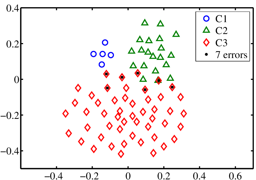
The row vectors of sparse codes are demonstrated in Figure 5 and Figure 7. Usually, on each column of , only one value dominates, which indicates the cluster membership. The cross sections of these vectors at the end of each segment indicate the overlapping regions. In Figure 5, the cross sections become more and more significant from (a) to (c), faithfully reflecting the overlapping status. Samples in these cross sections will be misclassified by Scut, which are plotted as black dots in Figure 4 and Figure 7.
The column vectors of sparse codes, taking G2 as example, are illustrated in Figure 8. For SSRk, compared with the original data in Figure 4(b), the codes make the cluster structure prominent. Besides, in contrast to the 0-1 discrete codes of K-means, the sparse codes are continuous, which can describe the clusters (if one entry dominates) and the overlaps (if several comparable entries exist). The truncated sparse codes try to resolve the overlaps, being closer to the K-means’s codes.
The Gram matrix reveals the linear relation of data: each sample can be approximated by the linear combination of all samples, with weights provided by the corresponding column of . Taking G2 as example, the matrices are shown in Figure 9. We see the weights in each column of distribute according to the relevance of the corresponding sample to all samples. removes the small weights, especially the negative ones, making the main relation clearer. For SSRk, the averages of column sums in on G1-G3 and onion are 1, 0.9866, 0.9249, and 0.9784 respectively, still close to 1, implying the distortions due to truncations are small.


| (%) | G1 | G2 | G3 | onion | iris | wdbc | Isolet | USPS3 | USPS8 | USPS10 | 4News | TDT2 |
|---|---|---|---|---|---|---|---|---|---|---|---|---|
| SSRl | 20.1 | 15.8 | 12.7 | 15.2 | 1.3 | 13.2 | 0.1 | 2.2 | 1.0 | 0.1 | 4.0 | 0.04 |
| SSRk | 100.0 | 59.4 | 58.4 | 39.4 | 63.2 | 67.7 | 16.8 | 60.5 | 5.1 | 6.8 | 1.9 | 4.7 |
| Accuracy (%) | Linear version | Kernel version | ||||
|---|---|---|---|---|---|---|
| Kmeans | K-PC | Rcutl | Scutl | Rcut | Scut | |
| G1 | 91.0 / 18.5 | 93.5 / 15.9 | 97.6 / 10.6 | 100.0 | 91.4 / 17.6 | 100.0 |
| G2 | 95.3 / 0.0 | 95.3 / 0.0 | 96.0 / 0.0 | 95.3 | 90.8 / 8.3 | 92.7 |
| G3 | 82.7 / 0.0 | 82.7 / 0.0 | 82.7 / 0.0 | 83.3 | 82.0 / 0.0 | 82.0 |
| onion | 61.7 / 6.9 | 62.5 / 7.2 | 62.6 / 5.2 | 61.3 | 90.5 / 6.6 | 90.7 |
| iris | 81.5 / 13.9 | 80.8 / 13.9 | 77.3 / 0.0 | 78.0 | 87.4 / 9.1 | 95.3 |
| wdbc | 85.4 / 0.0 | 85.4 / 0.0 | 85.4 / 0.0 | 87.5 | 88.9 / 0.0 | 88.4 |
| Isolet | 71.7 / 4.9 | 70.8 / 5.6 | 71.9 / 4.6 | 65.0 | 65.0 / 7.5 | 82.0 |
| USPS3 | 92.0 / 0.0 | 78.3 / 0.0 | 71.7 / 0.0 | 72.6 | 97.2 / 8.6 | 99.2 |
| USPS8 | 74.7 / 6.3 | 74.3 / 3.5 | 74.2 / 3.8 | 76.3 | 74.1 / 10.6 | 91.0 |
| USPS10 | 65.6 / 2.8 | 61.8 / 4.0 | 65.5 / 1.5 | 64.9 | 66.6 / 8.8 | 66.4 |
| 4News | 88.3 / 10.4 | 88.7 / 6.7 | 82.3 / 15.0 | 94.9 | 91.8 / 10.0 | 96.0 |
| Average | 80.9 / 5.8 | 79.5 / 5.2 | 78.8 / 3.7 | 79.9 | 84.2 / 7.9 | 89.4 |
7.3 Linear Version v.s. Kernel Version
We first compare how well the ideal graph condition is met for the two versions qualitatively from the view of the structure of similarity matrix, and then propose a measure for quantitative evaluation. Finally we compare the clustering performance of the two versions.
First, a clearer block-diagonal structure of the similarity matrix indicates the condition is met better. The similarity matrices on some representative data sets are shown in Figure 10. We see that so long as the data has clear clusters, the similarity matrix of the kernel version will meet the condition well, but that of the linear version does not necessarily be so. In Figure 10 (a)-(c), the condition is deviated more and more for the linear version, as can be expected from the data distributions of these data sets (see Figure 4(b) and Figure 11).
Next, based on the eigengap (Davis-Kahan) theorem of matrix perturbation (see Theorem 7 of [64]), we propose a value, measuring how well the ideal graph condition is met. The value of a similarity matrix for clusters is defined as
| (60) |
where is the th smallest eigenvalue of the Laplacian matrix. If , is defined to be 0. It has the following properties:
Theorem 20.
, and if and only if the ideal graph condition is met exactly.
Proof.
When the ideal graph condition is met, according to the properties of Laplacian matrix in Section 3.3, and , so . Conversely, if , then and , implying connected components exist, so the ideal graph condition is met. ∎
When the graph is nearly ideal, . The better the condition is met, the higher the is. A comparison of the values between the linear version and kernel version are shown in Table 3. It is clear that generally the kernel version meets the condition better than the linear version.
Finally, the clustering performance are compared in Table 4. The results on TDT2 and polb are absent, since the linear version fails to run on them. The kernel version generally performs better, for it meets the ideal graph condition better. The contrasts are most apparent on onion, iris, and wdbc, as implied by Figure 10. But, the results are reversed on G2 and G3, maybe the linear version meets the condition well (see Figure 10(a)).


7.4 Relations between , Sparsity of SSR, and Clustering Accuracy
In principle, reflects the separability of the clusters, it thus relates to the clustering accuracy. On the other hand, it implies the noise level in the indicator vectors, which is related to the sparsity of codes. Therefore, there are proportional relations between them. We validate the relations by a set of Gaussian data with more and more heavy overlaps (like G1-G3). The result is shown in Figure 13, clear proportional relations can be observed. The relations imply that, potentially, the value, which can be computed once the data is given, may provide us an estimation of the sparsity and the clustering performance before SSR and Scut are applied or when the ground-truth class labels are not available.
| Accuracy (%) | Graclus | Ncut | ZP | GMM-V | GMM | Kmeans | NJW | Rcut | Scut |
|---|---|---|---|---|---|---|---|---|---|
| G1 | 100.0 | 100.0 | 100.0 | 100.0 | 100.0 | 100.0 | 100.0 | 100.0 | 100.0 |
| G2 | 92.7 | 93.3 | 92.7 | 93.3 | 96.0 | 95.3 | 92.7 | 92.7 | 92.7 |
| G3 | 84.0 | 81.3 | 81.3 | 81.3 | 54.7 | 82.7 | 81.3 | 82.0 | 82.0 |
| onion | 62.7 | 90.7 | 90.7 | 73.3 | 93.3 | 57.3 | 90.7 | 92.0 | 90.7 |
| iris | 87.3 | 87.3 | 88.0 | 84.0 | 52.7 | 89.3 | 90.0 | 90.0 | 95.3 |
| wdbc | 88.4 | 77.7 | 88.2 | 83.5 | 85.1 | 85.4 | 81.9 | 88.9 | 88.4 |
| Isolet1 | 76.8 | 80.9 | 70.7 | 73.5 | 55.6 | 81.4 | 80.5 | 82.2 | 82.0 |
| USPS3 | 99.5 | 60.9 | 99.2 | 99.2 | 95.7 | 92.0 | 99.2 | 99.1 | 99.2 |
| USPS8 | 80.2 | 47.9 | 92.1 | 85.7 | 67.8 | 72.2 | 90.8 | 93.3 | 91.0 |
| USPS10 | 78.9 | 67.3 | 64.6 | 75.8 | 49.4 | 67.8 | 66.5 | 66.8 | 66.4 |
| 4News | 95.6 | 96.1 | 95.7 | 71.3 | - | 92.2 | 96.1 | 95.8 | 96.0 |
| TDT2 | 54.4 | 88.0 | 84.4 | 71.6 | - | - | 70.7 | 76.6 | 88.5 |
| polb | 83.8 | 82.9 | 84.8 | 81.0 | - | - | 82.9 | 87.6 | 84.8 |
| Average | 83.4 | 81.1 | 87.1 | 82.6 | 75.0 | 83.2 | 86.4 | 88.2 | 89.0 |
| NMI (%) | Graclus | Ncut | ZP | GMM-V | GMM | Kmeans | NJW | Rcut | Scut |
|---|---|---|---|---|---|---|---|---|---|
| G1 | 100.0 | 100.0 | 100.0 | 100.0 | 100.0 | 100.0 | 100.0 | 100.0 | 100.0 |
| G2 | 76.4 | 78.5 | 75.5 | 78.5 | 83.9 | 80.9 | 75.5 | 75.5 | 75.5 |
| G3 | 56.9 | 49.4 | 49.4 | 49.6 | 26.2 | 48.6 | 49.4 | 50.8 | 50.4 |
| onion | 44.6 | 68.4 | 68.4 | 37.9 | 74.4 | 46.4 | 68.4 | 71.4 | 68.4 |
| iris | 75.0 | 75.0 | 75.6 | 72.2 | 65.4 | 75.8 | 77.8 | 77.8 | 84.6 |
| wdbc | 49.4 | 35.2 | 49.0 | 42.5 | 37.1 | 46.7 | 39.2 | 49.9 | 49.4 |
| Isolet1 | 79.8 | 88.0 | 82.0 | 83.6 | 62.7 | 84.8 | 87.8 | 87.6 | 88.2 |
| USPS3 | 97.2 | 58.5 | 95.8 | 95.7 | 84.6 | 80.0 | 95.8 | 95.4 | 95.8 |
| USPS8 | 85.8 | 66.9 | 86.8 | 83.7 | 55.7 | 70.5 | 85.6 | 87.2 | 86.2 |
| USPS10 | 81.0 | 80.1 | 77.6 | 79.0 | 41.0 | 64.0 | 78.6 | 78.8 | 78.4 |
| 4News | 84.3 | 85.7 | 84.2 | 65.1 | - | 81.4 | 85.7 | 84.8 | 85.4 |
| TDT2 | 74.2 | 85.5 | 83.1 | 76.1 | - | - | 80.8 | 83.5 | 85.0 |
| polb | 55.4 | 54.2 | 58.6 | 57.8 | - | - | 54.2 | 65.1 | 58.6 |
| Average | 73.8 | 71.2 | 75.8 | 70.9 | 63.1 | 70.8 | 75.3 | 77.5 | 77.4 |
| RI (%) | Graclus | Ncut | ZP | GMM-V | GMM | Kmeans | NJW | Rcut | Scut |
|---|---|---|---|---|---|---|---|---|---|
| G1 | 100.0 | 100.0 | 100.0 | 100.0 | 100.0 | 100.0 | 100.0 | 100.0 | 100.0 |
| G2 | 90.8 | 91.6 | 90.8 | 91.6 | 94.8 | 94.0 | 90.8 | 90.8 | 90.8 |
| G3 | 81.7 | 79.0 | 79.0 | 78.6 | 56.7 | 79.7 | 79.0 | 79.2 | 79.6 |
| onion | 66.7 | 85.3 | 85.3 | 63.8 | 88.7 | 64.1 | 85.3 | 86.5 | 85.3 |
| iris | 86.2 | 86.2 | 86.8 | 83.7 | 72.2 | 88.0 | 88.6 | 88.6 | 94.2 |
| wdbc | 79.5 | 65.3 | 79.2 | 72.4 | 74.5 | 75.0 | 70.3 | 80.3 | 79.5 |
| Isolet1 | 96.7 | 97.5 | 95.6 | 96.2 | 93.1 | 97.3 | 97.4 | 97.2 | 97.5 |
| USPS3 | 99.4 | 73.9 | 99.0 | 98.9 | 95.0 | 90.8 | 99.0 | 98.9 | 99.0 |
| USPS8 | 94.6 | 83.1 | 96.4 | 95.7 | 88.1 | 91.5 | 96.2 | 96.8 | 96.0 |
| USPS10 | 94.6 | 93.5 | 92.9 | 94.6 | 78.8 | 91.7 | 93.3 | 93.2 | 93.2 |
| 4News | 95.7 | 96.2 | 95.8 | 83.6 | - | 92.5 | 96.2 | 95.9 | 96.1 |
| TDT2 | 91.3 | 96.3 | 95.3 | 93.7 | - | - | 93.8 | 95.1 | 96.2 |
| polb | 83.6 | 83.1 | 85.0 | 81.4 | - | - | 83.1 | 86.6 | 85.0 |
| Average | 82.4 | 87.0 | 90.9 | 87.2 | 84.2 | 87.7 | 90.2 | 91.5 | 91.7 |
| Time (s) | Graclus | Ncut | ZP | GMM-V | GMM | Kmeans | NJW | Rcut | Scut |
|---|---|---|---|---|---|---|---|---|---|
| USPS10 | 7.5 | 8.2 | 12.0 | 11.0 | 101.0 | 8.7 | 7.9 | 7.9 | 8.0 |
| 4News | 1.1 | 1.1 | 1.5 | 1.5 | - | 584.7 | 1.1 | 1.4 | 1.5 |
| TDT2 | 17.7 | 19.7 | 187.8 | 47.1 | - | - | 22.8 | 22.7 | 19.3 |
| Time (s) | ZP | GMM-V | NJW | Rcut | Scut |
|---|---|---|---|---|---|
| USPS10 | 4.20 | 3.13 | 0.08 | 0.10 | 0.12 |
| 4News | 0.05 | 0.06 | 0.01 | 0.01 | 0.05 |
| TDT2 | 168.80 | 28.10 | 2.66 | 3.69 | 0.34 |
7.5 Clustering via Kernel Scut
Since the superiority of kernel version has been demonstrated in previous section, now we focus on kernel Scut and compare it with some popular algorithms.
The results of accuracy, NMI, and RI are shown in Table 5.1717 17 Codes of Graclus and Ncut are downloaded from http://www.cs.utexas.edu/users/dml/Software/graclus.html and http://www.cis.upenn.edu/~jshi/software/ respectively. GMM and Kmeans are provided by MATLAB toolbox. The remaining methods are implemented by us using MATLAB. GMM cannot run on 4News and TDT2 due to , and Kmeans fails to run on TDT2. According to the mean scores of the three criteria, Scut performs best overall. Although the scores of Rcut are comparable to those of Scut, they are the best ones picked over 20 trials, the mean scores of Rcut are much worse, and the variances are large, as shown in Table 4. The difference between Rcut and Scut is that Rcut employs Kmeans to recover the indicators, while Scut employs NSCrt. In view of the comparable results of Scut to the optimal results of Rcut, it probably indicates that NSCrt has accurately recovered the underlying indicators. ZP and Ncut address similar problems too, especially ZP, which tries to recover indicators via rotation as NSCrt does. However, the results show that they do not perform as well as Scut. Graclus occasionally does best on some data sets, however, it performs poorly on some well-separable data sets, e.g., onion, iris, and TDT2.
The time cost on the three largest data sets, USPS10, 4News, and TDT2, is shown in Table 6. GMM and Kmeans are much slower. Scut is comparable to the most efficient method, Graclus. Designed to improve the computational cost of traditional spectral clustering methods, Graclus avoids the computation of eigenvectors. However, the total time cost of those methods working with similarity matrix, including Scut and Graclus, is dominated by the construction of similarity matrix. As a consequence, the cost of Scut is still close to that of Graclus. Table 6(b) highlights the cost of the post-processing of eigenvectors. On the largest data set TDT2, Scut is significantly faster than the others, since the time complexity of Scut is scaling linearly with data size.
Finally, as popular application of spectral clustering, image segmentation is compared between Rcut, Graclus, Ncut, and Scut. Results on two typical images are shown in Figure 14. The images and their similarity matrices are obtained from the web site of Ncut: http://www.cis.upenn.edu/~jshi/software/.
| Accuracy (%) | G1 | G2 | G3 | onion | iris | wdbc | Isolet | USPS3 | USPS8 | USPS10 |
|---|---|---|---|---|---|---|---|---|---|---|
| KSVD | 95.9 | 86.0 | 67.5 | 64.7 | 62.6 | 66.5 | 56.3 | 67.9 | 57.2 | 49.2 |
| SSC | 100.0 | 66.7 | 53.3 | 60.0 | 78.0 | 87.3 | 78.8 | 59.0 | - | - |
| Scutl | 100.0 | 95.3 | 83.3 | 61.3 | 78.0 | 87.5 | 65.0 | 72.6 | 76.3 | 64.9 |
| Accuracy (%) | G1 | G2 | G3 | onion | iris | wdbc | Isolet | USPS3 | USPS8 | USPS10 |
|---|---|---|---|---|---|---|---|---|---|---|
| KSVD | 91.3 | 93.3 | 74.7 | 58.7 | 82.0 | 67.0 | 23.9 | 43.1 | 19.7 | 17.5 |
| Scut | 100.0 | 92.7 | 82.0 | 90.7 | 95.3 | 88.4 | 82.0 | 99.2 | 91.0 | 66.4 |
7.6 OSRs v.s. SSR on clustering
We compare the two most related OSRs: KSVD and SSC [27], with SSR on clustering. Below, absence of results on 4News and TDT2 are due to running out of memory of KSVD and SSC.
First, for KSVD, we learn a dictionary and codes with the same sizes as SSRl, and apply the same clustering strategy as Scut.1818 18 The maximal -norm of KSVD is set to be . Considering KSVD depends on random initialization, it is repeated 20 times, and the mean accuracy is reported, since there is no suitable criterion to pick the optimal result. Codes of SSC is the ADMM version downloaded from http://www.cis.jhu.edu/~ehsan/code.htm. Independent affine subspaces is assumed for better performance. The results are shown in Table 7. Scutl outperforms KSVD and SSC significantly. Next, we learn an over-complete KSVD and apply K-means on the codes.1919 19 The number of atoms and the maximal -norm are set to be and respectively. Comparing with kernel Scut, the clustering results are shown in Table 8. Scut still performs better.
To investigate the reason of the inferior performance of KSVD against SSR, we compare how well the cluster structure of data is enhanced by the two kinds of sparse codes. This is measured by the ratio of within-class distance, , where is the mean of class , and is the mean of the whole set. The ratio is between 0 and 1. Smaller value implies better separability. In the same setting as last experiment, the ratios are shown in Figure 13. We see that the ratios of SSR are generally smaller than those of original data, which means SSR enhances the cluster structure. However, those of KSVD are significantly larger, implying the codes of KSVD are dispersed, which may not suitable for clustering purpose.


8 Extended Relations to Other Methods
We have established the inherent relations between PCA/LE, K-means/Rcut, and SSR so far. In this section, we will further link the framework to OSRs, kernel PCA, manifold learning, and subspace clustering.
8.1 Relation between OSRs and SSRl
We focus on two classical OSRs: [49] and KSVD [2], and compare them with SSRl. The relation will be explored mainly from the row-space view, rather than the column-space view that is sample-wise. It will be shown that the commonality of the methods is to find a sparse basis that covers the row space of data as much as possible. The sparse basis consists of the row vectors of the code matrix. The basis size can be chosen differently, whose range lies in . OSRs and SSRl occupy different sections of the range, that is where the difference comes from, and it leads to distinct solution strategies.
The objectives of [49] and KSVD are
| (61) |
| (62) |
respectively, where, , i.e., over-complete. We assume in this discussion .
Due to implicit sparsity constraint, the objective of SSRl can be expressed as
| (63) |
where , i.e., usually under-complete.
Fixing , . Substituting it into the objectives, all of them reduce to
| (64) |
with various sparse constraints on . Since is a projection matrix formed by the row vectors of , the above objective can be interpreted as: to find a sparse basis so that it covers the row space of data as much as possible. This is the common point of the three SRs.
The sparse basis of SSRl is obtained via rotating the normalized PCs (attached with ), showing a close tie to PCA. SSRl is also related to cluster analysis, due to the one-one correspondence between the normalized PCs and the eigenvectors of a linear Laplacian matrix. The basis size of SSRl is limited by the number of PCs, or equivalently the effective eigenvectors of Laplacian matrix. The over-completeness prevents OSRs from the reach of spectral graph theory as well as PCA, when . We do not know which vectors to draw from the void subspace that is complementary to the data row-space, so that attaching to the PCs and via rotation, they turn into sparse basis.
The dilemma is circumvented by resorting to the dictionary representation. Treating the dictionary and codes independently, OSRs obtain solution by alternate optimization. This strategy depends on a random initialization of the dictionary, which can be seen as replacing drawing vectors from the complementary row-subspace. The initialization is usually done via randomly drawing samples from the data set. Expressing , it is still not clear what the corresponding sparse codes are. However, if the dictionary is initialized with cluster centers, e.g., of K-means, the sparse codes are obviously the corresponding indicator vectors. Then following the alternate optimization, is fixed, the extreme sparse codes are relaxed and updated to soft ones, via some sample-wise sparse coding algorithms, e.g., OMP [50], BP [12], and then is updated and so on.2020 20 In KSVD, when the maximal -norm of codes is constrained to 1, KSVD reduces to vector quantization [32], and if further the nonzero value is constrained to be 1, it reduces to exactly K-means, as [2] had analyzed. The reverse process generalizes K-means to KSVD [2]. Notice that, K-means itself belongs to the SSR framework, while its solution adopts the alternate optimization. Unlike Rcut, K-means can obtain clusters more than the number of PCs. The cluster centers of K-means are usually initialized with random samples. Combining the two solution processes together, the above strategy is in fact K-means+OSR,2121 21 Similar strategies of clustering+OSR have been used in the proofs of exact dictionary recovery [1], showing some underlying relation between OSR and cluster analysis. in hindsight, it is interesting to find their counterpart PCA+SSR. At this point, the close ties between these methods are clear. A diagram is illustrated in Figure 1.
Further more, the four methods can be eventually unified at an extreme point, . At there is no choice, the whole complementary subspace has been included. A rotation of the full basis can lead to the ultimate sparse basis: the identity matrix. In this case, the dictionary consists of the whole data sets, with each sample serving as an atom/cluster center. They must be the optimal solution of OSRs and K-means too. This seemly useless extreme sparse representation had found its application in face recognition [69].
Finally, we comment that attributing to the random initialization, the formal relation of OSRs to cluster analysis is less obvious than that of SSRl, except a special case of KSVD; and the clustering performance of KSVD is not satisfactory as the experiments demonstrated. Nevertheless, the basis size SSRl can handle is limited, and OSRs had demonstrated impressive performance on signal denoising and reconstruction [25]. As sparse representation methods, SSRl and OSRs occupy different ranges and complement each other.
8.2 Relations between Kernel PCA, Manifold Learning, and SSR
First, we will show that kernel PCA (KPCA) [57] can be incorporated into the framework of SSR. The underlying reason is simple: PCA constitutes a part of SSR framework, and KPCA can be seen as a PCA, with original data replaced by high-dimensional features. Next, the relation is extended to manifold learning, including multidimensional scaling (MDS) [16], Isomap [62], and locally linear embedding (LLE) [53].
Let be a kernel matrix, and assume to find normalized PCs, the objective of KPCA is
Then we have
Theorem 21.
There is a sparse representation of KPCA: , where are the eigenvectors of KPCA.
Proof.
Assume LE uses the same kernel matrix, and the original data is not mean-removed, then PCA, KPCA, and LE can be seen as working with the following three similarity matrices respectively: , , and , where , , and , ensure the nonnegativity of the corresponding similarity matrices. The solution of PCA is obtained from the eigenvectors of , while that of KPCA is obtained from the eigenvectors of . By the correspondence between and , following the conversion from PCA to SSRl, the assertion is established. ∎
It implies KPCA is inherently related to cluster analysis too. We may wonder to what extent does KPCA reveal cluster structure, and how the clustering performance will be when using Scut. These questions can be answered by the ideal graph condition. Following the analysis of SSRl, we expect the similarity matrix used by KPCA meets the condition better than that used by PCA while worse than that used by LE. Though not reported, our experiments validated this. Besides, we mention that a significant drawback of KPCA is that it demands a large storage when dealing with large data sets, due to the dense kernel matrix.
Once KPCA has jointed the SSR framework, a series of manifold learning [33] or graph embedding [70] methods, including MDS, Isomap, and LLE, subsequently share extended relations to SSR. It is because, under a kernel view, these methods can be written into the form of KPCA, as is well-known in the literature [33, 6, 70]. In particular, it had been proven that classical MDS using Euclidean distance is exactly equivalent to PCA [67]. For metric MDS, Isomap (a special metric MDS that uses geodesic manifold distances), and LLE, relations to KPCA exist, although less rigorous, due to the kernel functions of their constructed “kernel matrices” are ambiguous [33].
Finally, it should be clarified that when we talk about the relations, it does not mean that dimensionality reduction or manifold learning is always related to SSR or cluster analysis. When the data do not exhibit cluster structure, these methods work as usual, and the codes preserve the data proximity. When clusters emerge in the data distribution, noisy or not, the codes are intrinsically embedded with cluster structure. Depending on two things, the structure becomes explicit: the attachment of vector and a proper rotation. We believe that for most real-world data, some underlying clusters naturally exist, more or less, and in a hierarchical way. Therefore, the codes must generally contain some cluster information, and the link of dimensionality reduction or manifold learning methods to SSR and cluster analysis should be commonplace. This explains why in so many paper focusing on manifold learning, the codes, when reduced to two dimensions for visualization, frequently exhibit a triangle shape (three clusters, cf. Figure 8). Plenty of examples can be found, e.g., in [55, 60, 56].
8.3 Relations between Subspace Clustering, LLE, and SSRl
A series of work in subspace clustering, represented by SSC [27], low-rank representation (LRR) [40], and the manifold learning method LLE [53] center around the seemingly trivial data representation form , which has been repeatedly interpreted in PCA, K-means, and SSR. We will show that SSC, LRR, LLE, and SSRl are related to each other, and the ideal graph condition is a special case of the ideal working condition of subspace clustering.
In cluster analysis, besides the clusters formed by spatial proximity, there is another circumstance that the clusters are formed by a union of linear subspaces, with one subspace corresponding to one cluster. The latter case is the subject of subspace clustering [63], which has found applications in, e.g., motion and image segmentation, face recognition [27, 40]. SSRl/Scutl may belong to this domain too. The ideal graph condition of linear version requires that the clusters should be orthogonal.2222 22 In this section, for SSRl, we consider the augmented data. For SSC and LRR, we focus on their basic models. This is a special case of the ideal working condition of subspace clustering, i.e., the subspaces being linearly independent.
The first step of SSC, LRR, LLE, and SSRl can be viewed as finding some code matrix to represent the data matrix with respect to a dictionary composed of the data matrix itself, i.e., solving with some constraint on . The problem is generally under-determined, with infinitely many solutions achieving zero error, e.g., the identity matrix and the Gram matrix , where is the full normalized PCs of data. SSC finds a sparse solution with the constraint that the diagonal being zero, i.e., forbidding self-representation. LRR finds a low-rank solution via minimizing the nuclear norm of , which turned out to be uniquely. LLE finds a sparse solution such that the nonzero entries of each column are constrained to the neighborhood of the associated point, and they sum to 1, i.e., each point is approximated locally by its neighborhood. For SSRl, we have . Note , which is the Gram matrix of PCs. SSC and LRR can achieve zero reconstruction error while SSRl is optimal within rank- limitation.
In the second step, SSC, LRR, and SSRl aim at clustering, while LLE is oriented to dimensionality reduction. When the subspaces are independent, [27] (excluding minor factors) and [40] proved their solutions are block-diagonal, if the data are arranged orderly. That is each point can be exactly reconstructed by its subspace. When the subspaces are orthogonal as the ideal graph condition requires, it is easy to see that all code matrices of the four methods become block-diagonal. Block-diagonal property is desirable, since it suits for the clustering purpose. In the second step of SSC and LRR, a similarity matrix is heuristically built based on , e.g., in SSC, then spectral clustering is employed to finish clustering. Since the code matrices are block-diagonal, so are the similarity matrices. It implies an ideal graph condition of kernel version is satisfied, making spectral clustering easy. For SSRl, this step can be omitted and clustering can be done by applying Scutl on , since the code matrix itself is a qualified similarity matrix, and the eigenvectors of the associated Laplacian matrix is exactly . In the second step of LLE, it seeks low-dimensional codes , such that it replaces original data and the neighborhood structure of data is preserved: , s.t. . For SSRl, this step can be omitted too, since itself is the codes and also the solution of LLE’s objective when .
Although LLE is designed for dimensionality reduction, by the same principle of SSC and LRR, it can be used for clustering too. Conversely, following LLE, SSC and LRR can be used for dimensionality reduction, regardless of the clusters. But only SSRl covers both domains in a natural way. We again witness the ambiguous borders between dimensionality reduction, sparse representation, and cluster analysis.
9 Conclusion and Future Work
In this paper, we have established a spectral graph-based framework unifying dimensionality reduction, cluster analysis, and sparse representation. It includes the inherent relations between PCA, K-means, LE, Rcut, SSR, and extended relations to OSRs, manifold learning, and subspace clustering. Based on the unification of PCA, K-means, LE, Rcut, a new sparse representation, SSR, has been derived. An efficient algorithm, NSCrt, has been developed to solve the sparse codes of SSR. As an application of SSR, the new clustering algorithm Scut achieved the state-of-the-art performance in the spectral clustering family.
The future work may include as follows. First, the theoretical analysis of whether NSCrt has the ability to recover underlying solution remains an open question. It is essentially a dictionary recovery problem. Recent results have shed light on it, e.g., [61, 1, 3]. Especially, [61] deals with square dictionary, and they proved that in noise-free case the dictionary can be recovered with high probability when each column of the codes has at most nonzeros and there are at least samples. It matches our case closely. Second, this paper remains in the unsupervised learning domain. It is interesting to find out whether the supervised classification can be incorporated into the spectral graph framework. Finally, in view of the relations of SSR to many other methods, as well as the nice properties it has, we envision that SSR may have other potential applications, especially the out-of-sample case.
Appendix A An Interpretation for Kernel Scut
In SSRk, Scut can be interpreted as clustering data according to the smallest included angle (or distance) between the cluster centers and the virtual data. By Theorem 14, the atoms of are cluster centers that are near-orthogonal and have similar lengths. In this case, it can be proved that
| (65) | ||||
which implies Scut performs clustering based on the smallest included angle.
Besides, since , Scut can also be interpreted as clustering data according to the smallest distance to the cluster centers.
References
- [1] Alekh Agarwal, Animashree Anandkumar, and Praneeth Netrapalli. Exact recovery of sparsely used overcomplete dictionaries. Arxiv, 2013.
- [2] Michal Aharon, Michael Elad, and Alfred Bruckstein. K-SVD: An algorithm for designing overcomplete dictionaries for sparse representation. IEEE Transactions on Signal Processing, 54(11):4311–4322, 2006.
- [3] Sanjeev Arora, Rong Ge, and Ankur Moitra. New algorithms for learning incoherent and overcomplete dictionaries. In Conference on Learning Theory, volume 35, pages 779–806, 2014.
- [4] Mikhail Belkin and Partha Niyogi. Laplacian eigenmaps for dimensionality reduction and data representation. Neural Computation, 15(6):1373–1396, 2003.
- [5] Yoshua Bengio, Olivier Delalleau, Nicolas Le Roux, Jean-François Paiement, Pascal Vincent, and Marie Ouimet. Learning eigenfunctions links spectral embedding and kernel PCA. Neural Computation, 16(10):2197–2219, 2004.
- [6] Yoshua Bengio, Jean-François Paiement, Pascal Vincent, Olivier Delalleau, Nicolas Le Roux, and Marie Ouimet. Out-of-sample extensions for lle, isomap, mds, eigenmaps, and spectral clustering. In Advances in Neural Information Processing Systems, volume 16, page 177. MIT Press, 2004.
- [7] Christopher M Bishop. Pattern Recognition and Machine Learning. Springer New York, 2006.
- [8] Y-Lan Boureau, Francis Bach, Yann LeCun, and Jean Ponce. Learning mid-level features for recognition. In IEEE Conference on Computer Vision and Pattern Recognition, pages 2559–2566. IEEE, 2010.
- [9] Alfred M Bruckstein, David L Donoho, and Michael Elad. From sparse solutions of systems of equations to sparse modeling of signals and images. SIAM Review, 51(1):34–81, 2009.
- [10] Emmanuel J Candès and Michael B Wakin. An introduction to compressive sampling. IEEE Signal Processing Magazine, 25(2):21–30, 2008.
- [11] Pak K Chan, Martine DF Schlag, and Jason Y Zien. Spectral k-way ratio-cut partitioning and clustering. IEEE Transactions on Computer-Aided Design of Integrated Circuits and Systems, 13(9):1088–1096, 1994.
- [12] Scott Shaobing Chen, David L Donoho, and Michael A Saunders. Atomic decomposition by basis pursuit. SIAM Journal on Scientific Computing, 20(1):33–61, 1998.
- [13] Fan RK Chung. Spectral Graph Theory. American Mathematical Society, 1997.
- [14] Adam Coates and Andrew Y Ng. The importance of encoding versus training with sparse coding and vector quantization. In International Conference on Machine Learning, pages 921–928. ACM, 2011.
- [15] Michael B. Cohen, Sam Elder, Cameron Musco, Christopher Musco, and Madalina Persu. Dimensionality reduction for k-means clustering and low rank approximation. In Annual ACM on Symposium on Theory of Computing, pages 163–172, 2015.
- [16] Trevor F Cox and Michael AA Cox. Multidimensional scaling. Chapman and Hall, 2001.
- [17] Fernando De la Torre. A least-squares framework for component analysis. IEEE Transactions on Pattern Analysis and Machine Intelligence, 34(6):1041–1055, 2012.
- [18] Inderjit Dhillon, Yuqiang Guan, and Brian Kulis. A unified view of kernel k-means, spectral clustering and graph cuts. Technical Report No. UTCS TR-04-25, 2005.
- [19] Inderjit S Dhillon, Yuqiang Guan, and Brian Kulis. Weighted graph cuts without eigenvectors a multilevel approach. IEEE Transactions on Pattern Analysis and Machine Intelligence, 29(11):1944–1957, 2007.
- [20] Chris Ding and Xiaofeng He. K-means clustering via principal component analysis. In International Conference on Machine Learning, page 29. ACM, 2004.
- [21] Chris HQ Ding, Xiaofeng He, and Hongyuan Zha. A spectral method to separate disconnected and nearly-disconnected web graph components. In International Conference on Knowledge Discovery and Data Mining, pages 275–280. ACM, 2001.
- [22] Weisheng Dong, Xin Li, Lei Zhang, and Guangming Shi. Sparsity-based image denoising via dictionary learning and structural clustering. In IEEE Conference on Computer Vision and Pattern Recognition, pages 457–464, 2011.
- [23] David Leigh Donoho. Compressed sensing. IEEE Transactions on Information Theory, 52(4):1289–1306, 2006.
- [24] Carl Eckart and Gale Young. The approximation of one matrix by another of lower rank. Psychometrika, 1(3):211–218, 1936.
- [25] Michael Elad, Mario AT Figueiredo, and Yi Ma. On the role of sparse and redundant representations in image processing. Proceedings of the IEEE, 98(6):972–982, 2010.
- [26] Michael Elad, Peyman Milanfar, and Ron Rubinstein. Analysis versus synthesis in signal priors. Inverse Problems, 23(3):1–5, 2007.
- [27] Ehsan Elhamifar and Rene Vidal. Sparse subspace clustering: Algorithm, theory, and applications. IEEE Transactions on Pattern Analysis and Machine Intelligence, 35(11):2765–2781, 2013.
- [28] K. Engan, S. O. Aase, and J. Hakon Husoy. Method of optimal directions for frame design. In IEEE International Conference on Acoustics, Speech, and Signal Processing, volume 5, pages 2443–2446, 1999.
- [29] Martin Ester, Hans-Peter Kriegel, Jörg Sander, and Xiaowei Xu. A density-based algorithm for discovering clusters in large spatial databases with noise. In International Conference on Knowledge Discovery and Data Mining, volume 96, pages 226–231. AAAI Press, 1996.
- [30] Ky Fan. A generalization of tychonoff’s fixed point theorem. Mathematische Annalen, 142(3):305–310, 1961.
- [31] Shenghua Gao, Ivor Wai-Hung Tsang, and Liang-Tien Chia. Kernel sparse representation for image classification and face recognition. In European Conference on Computer Vision, pages 1–14. 2010.
- [32] Allen Gersho and Robert M. Gray. Vector quantization and signal compression. Springer, 159(1):407–485, 1992.
- [33] Jihun Ham, Daniel D. Lee, Sebastian Mika, and Bernhard Schölkopf. A kernel view of the dimensionality reduction of manifolds. In International Conference on Machine Learning, page 47, 2004.
- [34] Trevor Hastie, Robert Tibshirani, Jerome Friedman, and James Franklin. The elements of statistical learning: data mining, inference and prediction. The Mathematical Intelligencer, 27(2):83–85, 2005.
- [35] Xiaofei He and Partha Niyogi. Locality preserving projections. In Advances in Neural Information Processing Systems, volume 16, page 153. MIT Press, 2004.
- [36] Zhenfang Hu, Gang Pan, Yueming Wang, and Zhaohui Wu. Sparse principal component analysis via rotation and truncation. IEEE Transactions on Neural Networks and Learning Systems, 27(4):875–890, 2016.
- [37] IT Jolliffe. Principal Component Analysis. Springer, 2002.
- [38] Harold W Kuhn. The Hungarian method for the assignment problem. Naval Research Logistics Quarterly, 2(1-2):83–97, 1955.
- [39] Daniel D Lee and H Sebastian Seung. Learning the parts of objects by non-negative matrix factorization. Nature, 401(6755):788–791, 1999.
- [40] Guangcan Liu, Zhouchen Lin, Shuicheng Yan, Ju Sun, Yong Yu, and Yi Ma. Robust recovery of subspace structures by low-rank representation. IEEE Transactions on Pattern Analysis and Machine Intelligence, 35(1):171–184, 2013.
- [41] Jun Liu, Shuiwang Ji, and Jieping Ye. SLEP: Sparse Learning with Efficient Projections. Arizona State University, 2009.
- [42] James MacQueen. Some methods for classification and analysis of multivariate observations. In Proceedings of the Fifth Berkeley Symposium on Mathematical Statistics and Probability, pages 281–297, 1967.
- [43] Christopher D Manning, Prabhakar Raghavan, and Hinrich Schütze. Introduction to information retrieval, volume 1. Cambridge University Press, 2008.
- [44] Bojan Mohar. Some applications of Laplace eigenvalues of graphs. Springer, 1997.
- [45] Bojan Mohar and Y Alavi. The Laplacian spectrum of graphs. Graph theory, Combinatorics, and Applications, 2:871–898, 1991.
- [46] S. Nam, M. E. Davies, M. Elad, and R. Gribonval. The cosparse analysis model and algorithms. Applied and Computational Harmonic Analysis, 34(1):30–56, 2013.
- [47] Andrew Y Ng, Michael I Jordan, and Yair Weiss. On spectral clustering: analysis and an algorithm. Advances in Neural Information Processing Systems, 2:849–856, 2002.
- [48] Feiping Nie, Zinan Zeng, Ivor W Tsang, Dong Xu, and Changshui Zhang. Spectral embedded clustering: a framework for in-sample and out-of-sample spectral clustering. IEEE Transactions on Neural Networks, 22(11):1796–1808, 2011.
- [49] Bruno A. Olshausen and David J. Field. Emergence of simple-cell receptive field properties by learning a sparse code for natural images. Nature, 381(6583):607–609, 1996.
- [50] Yagyensh Chandra Pati, Ramin Rezaiifar, and PS Krishnaprasad. Orthogonal matching pursuit: Recursive function approximation with applications to wavelet decomposition. In Proceedings of the 27 th Annual Asilomar Conference on Signals, Systems, and Computers, pages 40–44. IEEE, 1993.
- [51] Ignacio Ramirez, Pablo Sprechmann, and Guillermo Sapiro. Classification and clustering via dictionary learning with structured incoherence and shared features. In IEEE Conference on Computer Vision and Pattern Recognition, pages 3501–3508. IEEE, 2010.
- [52] S. Ravishankar and Y. Bresler. Learning sparsifying transforms. IEEE Transactions on Signal Processing, 61(5):1072–1086, 2013.
- [53] Sam T Roweis and Lawrence K Saul. Nonlinear dimensionality reduction by locally linear embedding. Science, 290(5500):2323–2326, 2000.
- [54] Ron Rubinstein, Alfred M Bruckstein, and Michael Elad. Dictionaries for sparse representation modeling. Proceedings of the IEEE, 98(6):1045–1057, 2010.
- [55] Lawrence K. Saul and Sam T. Roweis. Think globally, fit locally: unsupervised learning of low dimensional manifolds. Journal of Machine Learning Research, 4(2):119–155, 2003.
- [56] Lawrence K Saul, Kilian Q Weinberger, Jihun H Ham, Fei Sha, and Daniel D Lee. Spectral methods for dimensionality reduction. Semisupervised Learning, pages 293–308, 2006.
- [57] Bernhard Schölkopf, Alexander Smola, and Klaus-Robert Müller. Nonlinear component analysis as a kernel eigenvalue problem. Neural Computation, 10(5):1299–1319, 1998.
- [58] John Shawe-Taylor and Nello Cristianini. Kernel methods for pattern analysis. Cambridge university press, 2004.
- [59] Jianbo Shi and Jitendra Malik. Normalized cuts and image segmentation. IEEE Transactions on Pattern Analysis and Machine Intelligence, 22(8):888–905, 2000.
- [60] Vin De Silva and Joshua B. Tenenbaum. Global versus local methods in nonlinear dimensionality reduction. In Advances in Neural Information Processing Systems, volume 15, pages 1959 – 1966, 2003.
- [61] Daniel A. Spielman, Huan Wang, and John Wright. Exact recovery of sparsely-used dictionaries. In Conference on Learning Theory, volume 23, 2012.
- [62] Joshua B Tenenbaum, Vin De Silva, and John C Langford. A global geometric framework for nonlinear dimensionality reduction. Science, 290(5500):2319–2323, 2000.
- [63] René Vidal. Subspace clustering. IEEE Signal Processing Magazine, 28(2):52–68, 2011.
- [64] Ulrike Von Luxburg. A tutorial on spectral clustering. Statistics and Computing, 17(4):395–416, 2007.
- [65] Fei Wang, Changshui Zhang, and Tao Li. Clustering with local and global regularization. IEEE Transactions on Knowledge and Data Engineering, 21(12):1665–1678, 2009.
- [66] Christopher K. I. Williams and Matthias Seeger. Using the nystrom method to speed up kernel machines. Advances in Neural Information Processing Systems, 13, 2001.
- [67] Christopher KI Williams. On a connection between kernel PCA and metric multidimensional scaling. Machine Learning, 46(1-3):11–19, 2002.
- [68] John Wright, Yi Ma, Julien Mairal, Guillermo Sapiro, Thomas S Huang, and Shuicheng Yan. Sparse representation for computer vision and pattern recognition. Proceedings of the IEEE, 98(6):1031–1044, 2010.
- [69] John Wright, Allen Y Yang, Arvind Ganesh, S Shankar Sastry, and Yi Ma. Robust face recognition via sparse representation. IEEE Transactions on Pattern Analysis and Machine Intelligence, 31(2):210–227, 2009.
- [70] Shuicheng Yan, Dong Xu, Benyu Zhang, Hong Jiang Zhang, Qiang Yang, and Stephen Lin. Graph embedding and extensions: A general framework for dimensionality reduction. IEEE Transactions on Pattern Analysis and Machine Intelligence, 29(1):40–51, 2007.
- [71] Jianchao Yang, Kai Yu, Yihong Gong, and Thomas Huang. Linear spatial pyramid matching using sparse coding for image classification. In IEEE Conference on Computer Vision and Pattern Recognition, pages 1794–1801. IEEE, 2009.
- [72] Zhirong Yang, Tele Hao, Onur Dikmen, Xi Chen, and Erkki Oja. Clustering by nonnegative matrix factorization using graph random walk. In Advances in Neural Information Processing Systems, pages 1088–1096, 2012.
- [73] Stella X Yu and Jianbo Shi. Multiclass spectral clustering. In IEEE International Conference on Computer Vision, pages 313–319. IEEE, 2003.
- [74] Ron Zass and Amnon Shashua. A unifying approach to hard and probabilistic clustering. In IEEE International Conference on Computer Vision, volume 1, pages 294–301. IEEE, 2005.
- [75] Lihi Zelnik-Manor and Pietro Perona. Self-tuning spectral clustering. In Advances in Neural Information Processing Systems, pages 1601–1608, 2004.