Modeling an elastic beam with piezoelectric patches by including magnetic effects

Piezoelectric materials have been successfully used to transfer mechanical energy into electro-magnetic energy, and vice versa. Due to their low cost, light weight, and high durability, they have been very competitive for many tasks in many fields ranging from space technology to the automotive industry. A single piezoelectric beam is an elastic beam covered by electrodes on its top and bottom surfaces, insulated at the edges (to prevent fringing effects), and connected to an external electric circuit. (See Figure 1.)

We use a variational approach to describe the dynamics for a piezoelectric beam with both Euler-Bernoulli and Mindlin-Timoshenko small displacement assumptions. Using the same methodology, we describe the dynamics for the common configuration of an elastic beam with two piezoelectric patches bonded on the elastic beam top and bottom surfaces as shown in Figure 2. Mechanical effects are modelled through Euler-Bernoulli (E-B) or Mindlin-Timoshenko (M-T) small displacement assumptions, for instance see [1], [3], [4], [13], [17]. The (M-T) model includes all the effects of the (E-B) model, and additionally, it includes the effects of the shear strain and rotational inertia. The (E-B) beam model is not sufficient to describe the dynamics of thin beams vibrating at high frequencies or of beams with low length-to-width aspect ratios (short and stubby beams), see [2] and the references therein. Our (M-T) model is different from the model in [19] where the degree of smoothness of the control operator is the same as that of the (E-B) model.

Most studies of piezoelectric structures consider only mechanical and electrical effects but not magnetic effects. Electrical and magnetic effects are modeled by Maxwell’s equations with three widely used assumptions: electro-static, quasi-static and fully dynamic [14]. Electro-static and quasi-static approaches are the most widely used, see for instance [5], [7], [12], [13], [14], [16]. Assuming stationary electrical effects is generally considered a reasonable assumption since it has been experimentally observed that magnetic effects are a very minor aspect of the overall dynamics for polarized ceramics, see the review article [18]. However, in [9], it is shown that the controlled piezoelectric beam with magnetic effects is not strongly stabilizable for many parameter values. This is quite different from the stabilizability and controllability of a piezoelectric beam without magnetic effects.

In this paper, we include all magnetic effects and model a beam-patch system driven by two different voltage sources. The dynamics of electro-magnetic effects are included. Hamilton’s Principle leads to strongly coupled equations for stretching and bending with the (E-B) assumptions, and for stretching, bending and rotation with the (M-T) assumptions. Conditions at the boundary of the patches are also obtained.

In this section we present the initial and boundary value problem for models of a piezoelectric beam that include full magnetic effects. Throughout this paper, we use dots and primes to denote differentiation with respect to time $(t)$ and space $(x),$ respectively. We first start with the modeling of piezoelectric patches. Let $x_{1},x_{2}$ be the longitudinal directions and let $x_{3}$ be transverse directions. We assume that the elastic beam occupies the region $\Omega=[0,L]\times[-r,r]\times[-\frac{h}{2},\frac{h}{2}].$ We denote by $\partial\Omega$ the boundary of $\Omega;$ the electroded region and the insulated region.

We adopt the following linear constitutive relationship [14] for piezoelectric beams

$\displaystyle\left(\begin{array}[]{l}T\\ D\\ \end{array}\right)=\left[{\begin{array}[]{*{20}c}c&-\Gamma^{\text{T}}\\ \Gamma&\varepsilon\\ \end{array}}\right]\left(\begin{array}[]{l}S\\ E\\ \end{array}\right)$

where $T=(T_{11},T_{22},T_{33},T_{23},T_{13},T_{12})^{\text{T}}$ is the stress vector, $S=(S_{11},S_{22},S_{33},S_{23},S_{13},S_{12})^{\text{T}}$ is the strain vector, $D=(D_{1},D_{2},D_{3})^{\text{T}}$ and $E=(E_{1},E_{2},E_{3})^{\text{T}}$ are the electric displacement and the electric field vectors, respectively, and moreover, the matrices $[c],[\Gamma],[\varepsilon]$ are the matrices with elastic, electro-mechanic and dielectric constant entries. (For more details, see [14].) Under the assumption of transverse isotropy and polarization in $x_{3}-$direction, these matrices reduce to $\varepsilon={\text{diag}}(\varepsilon_{1},\varepsilon_{2},\varepsilon_{3}),$ and

	$\displaystyle c=\left[{\begin{array}[]{*{20}c}{c_{11}}&{c_{12}}&{c_{13}}&0&0&0\\ {c_{21}}&{c_{22}}&{c_{23}}&0&0&0\\ {c_{31}}&{c_{32}}&{c_{33}}&0&0&0\\ 0&0&0&c_{44}&0&0\\ 0&0&0&0&c_{55}&0\\ 0&0&0&0&0&c_{66}\end{array}}\right],$
	$\displaystyle\Gamma=\left[{\begin{array}[]{*{20}c}0&0&0&0&\gamma_{15}&0\\ 0&0&0&-\gamma_{15}&0&0\\ \gamma_{31}&\gamma_{31}&\gamma_{33}&0&0&0\end{array}}\right].$

In standard beam theory, all forces acting in the $x_{2}$ direction, and the transverse normal stress $T_{33}$ are negligible. In (E-B) beam theory, the shear strain $S_{13}$ is zero but it is nonzero in (M-T) beam theory.

Denote flexural rigidity, modulus of elasticity, piezoelectric coefficients, and dielectric constants by $c_{11},c_{55},e_{31},e_{15},{\varepsilon_{1}}$ and ${\varepsilon_{3}}$, respectively. Let $v=v(x),$ $w=w(x)$ and $\psi=\psi(x)$ denote the longitudinal displacement of the center line, transverse displacement , and the rotation of the beam, respectively. For simplicity of notation we set $x=x_{1}$ and $z=x_{3}.$ Continuing with the small-displacement assumptions, the displacement fields, strains, and the linear constitutive equations [14] for the (E-B) and (M-T) beam models are given in Table I with the following notation

	$\displaystyle\gamma_{1}=\gamma_{15},~\gamma_{3}=\gamma_{31},~\alpha_{1}=\alpha_{11}+\gamma_{3}^{2}\beta_{3},~\beta_{1}=\frac{1}{\varepsilon_{1}}$
	$\displaystyle\alpha_{3}=\alpha_{11}+\gamma_{1}^{2}\beta_{1},~\alpha_{11}=c_{11},~~\alpha_{33}=c_{55},~\beta_{3}=\frac{1}{\varepsilon_{3}}.$		(19)

Electro-magnetic effects are described by Maxwell’s equations:

	$\displaystyle\nabla\cdot D=~\sigma_{b}$	$\displaystyle\quad{\rm{in}}\quad\Omega\times\mathbb{R}^{+}~$		(20a)
	$\displaystyle\nabla\cdot B=~0$	$\displaystyle\quad{\rm{in}}\quad\Omega\times\mathbb{R}^{+}~$		(20b)
	$\displaystyle\nabla\times E=~-\dot{B}$	$\displaystyle\quad{\rm{in}}\quad\Omega\times\mathbb{R}^{+}~$		(20c)
	$\displaystyle\frac{1}{\mu}(\nabla\times B)=~i_{b}+\dot{D}$	$\displaystyle\quad{\rm{in}}\quad\Omega\times\mathbb{R}^{+}~$		(20d)

where the dots denote differentiation with respect to time $t.$ Here $B$ denotes magnetic field vector, and $\sigma_{b},i_{b},\sigma_{s},i_{s},V,\mu,n$ denote body charge density, body current density, surface charge density, surface current density, voltage, magnetic permeability, and unit normal vector respectively. In this paper it is assumed that the only external force acting on the beam is the voltage applied at the electrodes and so the essential electric boundary conditions are

	$\displaystyle-D\cdot n=~\sigma_{s}$	$\displaystyle\quad{\rm{on}}\quad{\partial\Omega}\times\mathbb{R}^{+}~\quad$	(Charge )		(21a)
	$\displaystyle\frac{1}{\mu}(B\times n)=~i_{s}$	$\displaystyle\quad{\rm{on}}\quad{\partial\Omega}\times\mathbb{R}^{+}~\quad$	(Current)		(21b)
	$\displaystyle\phi=~V$	$\displaystyle\quad{\rm{on}}\quad{\partial\Omega}\times\mathbb{R}^{+}~\quad$	(Voltage).		(21c)

There are mainly three approaches to inclusion of electromagnetic effects in piezo-electric beams [14]:

In this paper, the third, fully dynamic approach for modeling piezoelectric beams that includes all of the magnetic effects, is used as in [9]. The magnetic field $B$ is perpendicular to the $x-y$ plane due to Gauss’s law of magnetism, i.e. $\nabla\cdot B=~0,$ and therefore $B=(B_{1},B_{2},B_{3})$ has only the $y-$component $B_{2}$ nonzero, and it is only a function of $x.$ This is because the surface current at the electrodes have only $x-$component (tangential) and $B$ is perpendicular to both the outward normal vector ($n=(0,0,1)$ or $n=(0,0,-1)$) at the electrodes and the current on the electrodes. For simplicity, we also assume that $E_{1}=0,$ and thus $D_{1}=0$ by Table I. Maxwell’s equations including the effects of $B$ become

$$\nabla\cdot B=0,~~~\dot{B}=-\nabla\times E,~~~\dot{D}=\frac{1}{\mu}(\nabla\times B).$$

From the last equation it follows that

$$\frac{dB_{2}}{dx}=-\mu\dot{D}_{3},$$

and so

$$B_{2}=-\mu\int\dot{D}_{3}(\xi,x_{3},t)~d\xi.$$

The next assumption is that $D_{3}$ is constant in $x_{3}:$ $D_{3}(x,x_{3},t)=D_{3}(x,t).$ Now let

$\displaystyle q=\int D_{3}(x,t)~dx$

(22)

so that $q^{\prime}=D_{3}$ and $-\mu\dot{q}=B_{2}.$ The magnetic energy (which can be regarded as the electric kinetic energy) is

$\displaystyle\mathbf{B}$

$\displaystyle=$

$\displaystyle\frac{1}{2\mu}\int_{\Omega}(B_{2})^{2}~dX=\frac{\mu}{2}\int_{\Omega}\dot{q}^{2}~dX.$

Since the voltage is prescribed at the electrodes, we use the Lagrangian [8, 9]

$\displaystyle\mathbf{L}=\int_{0}^{T}\left[\mathbf{K}-(\mathbf{P}+\mathbf{E})+\mathbf{B}+\mathbf{W}\right]~dt$

(23)

where $\mathbf{K},$ $\mathbf{P}+\mathbf{E},$ $\mathbf{B},$ and $\mathbf{W}$ denote the (mechanical) kinetic energy, total stored energy, magnetic energy (electrical kinetic energy) of the beam, and the work done by the external forces, respectively. This is different than that in [4] since that paper considers charge actuation. Using (22) and Table I, leads to the energies

		$\displaystyle\mathbf{P}+\mathbf{E}=\frac{1}{2}\int_{\Omega}\left(T_{11}S_{11}+D_{3}E_{3}\right)~dX$
		$\displaystyle~~=\frac{h}{2}\int_{0}^{L}\left[\alpha_{1}(v^{\prime 2}+\frac{h^{2}}{12}w^{\prime\prime 2})-2\gamma_{3}\beta_{3}v^{\prime}q^{\prime}+\beta_{3}q^{\prime 2}\right]dx,\hskip 9.24994pt\text{(E-B)}$
		$\displaystyle\mathbf{K}=\frac{\rho}{2}\int_{\Omega}\left(\dot{U}_{1}^{2}+\dot{U}_{3}^{2}\right)~dX$
		$\displaystyle~~=\frac{\rho h}{2}\int_{0}^{L}\left(\dot{v}^{2}+\frac{h^{2}}{12}\dot{w}^{\prime 2}+\dot{w}^{2}\right)~dx,\hskip 9.24994pt\text{(E-B)}$
		$\displaystyle\mathbf{P}+\mathbf{E}=\frac{1}{2}\int_{\Omega}\left(T_{11}S_{11}+T_{13}S_{13}+D_{3}E_{3}\right)~dX$
		$\displaystyle~~=\frac{h}{2}\int_{0}^{L}\left[\alpha_{1}\left(v^{\prime 2}+\frac{h^{2}}{12}\psi^{\prime 2}\right)+\alpha_{3}(w^{\prime}+\psi)^{2}\right.,$
		$\displaystyle\hskip 9.24994pt~~\left.-2\gamma_{1}\beta_{1}v^{\prime}q^{\prime}+\beta_{3}q^{\prime 2}-2\gamma_{1}\beta_{1}v^{\prime}q^{\prime}+\beta_{3}q^{\prime 2}\right]~dx,\hskip 9.24994pt\text{(M-T)}$
		$\displaystyle\mathbf{K}=\frac{\rho}{2}\int_{\Omega}\left(\dot{U}_{1}^{2}+\dot{U}_{3}^{2}\right)~dX$
		$\displaystyle~~=\frac{\rho h}{2}\int_{0}^{L}\left(\dot{v}^{2}+\frac{h^{2}}{12}\dot{\psi}^{2}+\dot{w}^{2}\right)~dx,\hskip 9.24994pt\text{(M-T)}$
		$\displaystyle\mathbf{B}=\frac{1}{2\mu}\int_{\Omega}\|B\|^{2}~dX=\frac{\mu h}{2}\int_{0}^{L}\dot{q}^{2}~dx,\text{(E-B), \text{(}M-T)}\hskip 9.24994pt$
		$\displaystyle\mathbf{W}=-\int_{\partial\Omega}D_{3}~\bar{\phi}~d\Gamma=-\int_{0}^{L}q^{\prime}~V(t)~dx,\text{(E-B), \text{(}M-T)}$		(24)

where $\bar{\phi}$ is the electric potential, and $V(t)$ is the voltage applied at the electrodes. Note that voltage $V(t)$ is the potential difference between the top and bottom electrodes.

Application of Hamilton’s principle, setting the variation of admissible displacements $\{v,w,q\}$ for (E-B) and $\{v,\psi,w,q\}$ of (M-T) of $\bf L$ to zero, yields three partial differential equations. If we assume that the beam is free at both ends $x=0,L,$ we obtain the sets of partial differential equations and boundary conditions for the (E-B) assumptions

		$\displaystyle\rho\ddot{v}-\alpha_{1}v^{\prime\prime}+\gamma_{3}\beta q^{\prime\prime}=0$		(25a)
		$\displaystyle\mu\ddot{q}-\beta_{3}v^{\prime\prime}+\gamma_{3}\beta_{3}q^{\prime\prime}=0\quad\text{(Stretching)}$		(25b)
		$\displaystyle\rho h\ddot{w}+\frac{\alpha_{1}h^{3}}{12}w^{\prime\prime\prime\prime}=0\quad\quad\text{(Bending)}$		(25c)
		$\displaystyle\left.~\alpha_{1}v^{\prime}-\gamma_{3}\beta_{3}q^{\prime}~\right|_{x=0,L}=0$		(25d)
		$\displaystyle\left.~\beta_{3}q^{\prime}-\gamma_{3}\beta_{3}v^{\prime}~\right|_{x=0,L}=-\frac{V(t)}{h}$		(25e)
		$\displaystyle w^{\prime\prime}(0)=w^{\prime\prime\prime}(0)=w^{\prime\prime}(L)=w^{\prime\prime\prime}(L)=0,$		(25f)

and for the (M-T) assumptions

		$\displaystyle\rho\ddot{v}-\alpha_{1}v^{\prime\prime}+\gamma_{3}\beta q^{\prime\prime}=0$		(26a)
		$\displaystyle\mu\ddot{q}-\beta_{3}v^{\prime\prime}+\gamma_{3}\beta_{3}v^{\prime\prime}=0\quad\text{(Stretching)}$		(26b)
		$\displaystyle\rho h\ddot{w}-\alpha_{3}h(\psi+w^{\prime})^{\prime}=0\quad\quad\text{(Bending)}$		(26c)
		$\displaystyle\frac{\rho h^{3}}{12}\ddot{\psi}-\frac{\alpha_{1}h^{3}}{12}\psi^{\prime\prime}$		(26d)
		$\displaystyle\quad\quad\quad+\alpha_{3}h(\psi+w^{\prime})=0\quad\text{(Rotation)}$		(26e)
		$\displaystyle\left.~\alpha_{1}v^{\prime}-\gamma_{3}\beta_{3}q^{\prime}~\right|_{x=0,L}=0$		(26f)
		$\displaystyle\left.~\beta_{3}q^{\prime}-\gamma_{3}\beta_{3}v^{\prime}~\right|_{x=0,L}=-\frac{V(t)}{h}$		(26g)
		$\displaystyle\left.\psi^{\prime},~(\psi+w^{\prime})~\right|_{x=0,L}=0.$		(26h)

Since the only external force acting on the beam is the voltage at the electrodes, the bending and rotation equations are completely decoupled from the stretching equations.

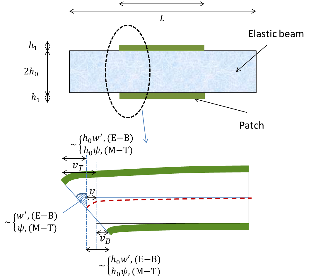
In this section, we consider an elastic beam of length $L$ and height $2h_{0}$ with two piezoelectric patches with height $h_{1}$ bonded one at the top and one at the bottom of the beam. Defining $\omega=[a,b]$ where $0<a<b<L,$ the symmetrically placed patches occupy the region $\Omega_{\omega}=\omega\times[-r,r]\times\left([-h_{0}-h_{1},-h_{0}]\bigcup[h_{0},h_{0}+h_{1}]\right)\subset\Omega.$ The patches are insulated at the edges, and no external mechanical stress is applied through the edges. They are also assumed to be bonded perfectly so that no slip occurs. Moreover, each patch is covered with electrodes at lower and upper faces (See Figure 2). The prescribed voltages at each patch can be different.

As shown in the previous section (see (25) and (26)), when the voltage is prescribed at a patch it either shrinks or extends, so we only consider the stretching motions for the patches. We use $v^{T}$ and $v^{B}$ to denote longitudinal displacements of the centerlines of the top and bottom patches, respectively, and $v,$ $w,$ and $\psi$ denote the longitudinal displacement of centerline, transverse displacement, and rotation respectively of the elastic beam. Let $V^{T}(t)$ and $V^{B}(t)$ indicate the applied voltages to the top and bottom piezoelectric patches.

Assuming that the patches are bonded firmly and there is no slipping, we have the following continuity relationship due to the geometry shown in Figure 3:

		$\displaystyle v^{T}=v+h_{0}w^{\prime},v^{B}=v-h_{0}w^{\prime},$	(E-B)		(27)
		$\displaystyle v^{T}=v+h_{0}\psi,~~v^{B}=v-h_{0}\psi.$	(M-T)		(28)

Letting the indices $b,T,B$ refer to the quantities of beam, top patch, and bottom patch, respectively, the total kinetic, potential, electric, magnetic energies and the work done by the external forces are

	$\displaystyle\tilde{\mathbf{K}}=\mathbf{K}^{b}+\mathbf{K}^{T}+\mathbf{K}^{B},~\tilde{\mathbf{P}}=\mathbf{P}^{b}+\mathbf{P}^{T}+\mathbf{P}^{B},$
	$\displaystyle~\tilde{\mathbf{E}}=\mathbf{E}^{T}+\mathbf{E}^{B},~\tilde{\mathbf{B}}=\mathbf{B}^{T}+\mathbf{B}^{B},~~\tilde{\mathbf{W}}=\mathbf{W}^{T}+\mathbf{W}^{B}.$

Assume that the material properties of the two patches are identical, and use the superscript $p$ to indicate the material property of a patch and $b$ to indicate the corresponding property of the beam. The magnetic energy and work done are

		$\displaystyle\mathbf{B}^{T}=\frac{1}{2\mu}\int_{\Omega_{\omega}}\|B^{T}\|^{2}~dX=\frac{\mu h}{2}\int_{\omega}(\dot{q}^{T})^{2}~dx$
		$\displaystyle\mathbf{B}^{B}=\frac{1}{2\mu}\int_{\Omega_{\omega}}\|B^{B}\|^{2}~dX=\frac{\mu h}{2}\int_{\omega}(\dot{q}^{B})^{2}~dx$
		$\displaystyle\mathbf{W}^{T}=\int_{\omega}-{q^{T}}^{\prime}~V^{T}(t)~dx$
		$\displaystyle\mathbf{W}^{B}=\int_{\omega}-{q^{B}}^{\prime}~V^{T}(t)~dx.\quad\text{(E-B), (M-T)}\quad\quad$

The kinetic energy of the beam and patches, potential energy of the beam, and the total stored energy of patches are

		$\displaystyle\mathbf{K}^{b}=\rho h_{0}\int_{0}^{L}\left(\dot{v}^{2}+\frac{h^{2}}{3}\dot{w}_{x}^{2}+\dot{w}^{2}\right)~dx$
		$\displaystyle\mathbf{K}^{T}+\mathbf{K}^{B}=\rho h_{1}\int_{\omega}\left[\left(\dot{v}+h_{0}\dot{w}^{\prime}\right)^{2}+\left(\dot{v}-h_{0}\dot{w}^{\prime}\right)^{2}\right]~dx$
		$\displaystyle\mathbf{P}^{b}=h_{0}\int_{0}^{L}\left(\alpha_{1}\left(v^{\prime 2}+\frac{h_{0}^{2}}{3}w^{\prime\prime 2}\right)\right)~dx$
		$\displaystyle\mathbf{P}^{T}+\mathbf{E}^{T}=\frac{h_{1}}{2}\int_{\omega}\left(\alpha_{1}^{p}(v^{\prime}+h_{0}w^{\prime\prime})^{2}\right.$
		$\displaystyle\left.\quad\quad\quad\quad\quad\quad-2\gamma_{3}\beta_{3}(v^{\prime}+h_{0}w^{\prime\prime})(q^{T})^{\prime}+\beta_{3}(q^{T})^{\prime 2}\right)~dx$
		$\displaystyle\mathbf{P}^{B}+\mathbf{E}^{B}=\frac{h_{1}}{2}\int_{\omega}\left(\alpha_{1}^{p}(v^{\prime}-h_{0}w^{\prime\prime})^{2}\right.$
		$\displaystyle\left.-2\gamma_{3}\beta_{3}(v^{\prime}-h_{0}w^{\prime\prime})(q^{B})^{\prime}+\beta_{3}(q^{B})^{\prime 2}\right)~dx,~~\text{(E-B)}\quad\quad$

and with (M-T) assumptions,

		$\displaystyle\mathbf{K}^{b}=\rho h_{0}\int_{0}^{L}\left(\dot{v}^{2}+\frac{h^{2}}{3}\dot{\psi}^{2}+\dot{w}^{2}\right)~dx$
		$\displaystyle\mathbf{K}^{T}+\mathbf{K}^{B}=\frac{\rho h_{1}}{2}\int_{\omega}\left[\left(\dot{v}^{2}+h_{0}\dot{\psi}\right)^{2}+\left(\dot{v}^{2}-h_{0}\dot{\psi}\right)^{2}\right]~dx$
		$\displaystyle\mathbf{P}^{b}=h_{0}\int_{0}^{L}\left(\alpha_{1}\left(v^{\prime 2}+\frac{h_{0}^{2}}{3}\psi^{\prime 2}\right)+\alpha_{3}(w^{\prime}+\psi)^{2}\right)~dx$
		$\displaystyle\mathbf{P}^{T}+\mathbf{E}^{T}=\frac{h_{1}}{2}\int_{\omega}\left(\alpha_{1}^{p}(v^{\prime}+h_{0}\psi^{\prime})^{2}\right.$
		$\displaystyle\left.\quad\quad\quad\quad\quad\quad-2\gamma_{3}\beta_{3}(v^{T})^{\prime}(q^{T})^{\prime}+\beta_{3}(q^{T})^{\prime 2}\right)~dx$
		$\displaystyle\mathbf{P}^{B}+\mathbf{E}^{B}=\frac{h_{1}}{2}\int_{\omega}\left(\alpha_{1}^{p}(v^{B})^{\prime 2}\right.$
		$\displaystyle\left.\quad\quad\quad\quad\quad-2\gamma_{3}\beta_{3}v^{B}(q^{B})^{\prime}+\beta_{3}(q^{B})^{\prime 2}\right)~dx.\quad\text{(M-T)}\quad\quad$

The Lagrangian corresponding to the whole beam-patch system (similar ro (23)) is

$\displaystyle\tilde{\mathbf{L}}=$

$\displaystyle\int_{0}^{T}\left[\tilde{\mathbf{K}}-(\tilde{\mathbf{P}}+\tilde{\mathbf{E}})+\tilde{\mathbf{B}}+\tilde{\mathbf{W}}\right]~dt.$

(29)

We set the variation of $\tilde{\mathbf{L}}$ with respect to all admissible displacements $\{v,w,q^{T},q^{B}\}$ for (E-B) and $\{v,w,\psi,q^{T},q^{B}\}$ for (M-T) to zero. Since the bonding is assumed to be perfect, we also use the constraints that $v,w$ and $w^{\prime}$ for (E-B) and $v,w$ and $\psi$ for (M-T) are continuous at the edges of the patches. Note that $q^{T}$ and $q^{B}$ are zero outside the region $\omega.$ Letting $\chi_{\omega}(x)$ indicate the characteristic function of the interval $\omega=(a,b),$ define

$$\rho(x)=h_{1}\rho^{p}\chi_{\omega}(x)+h_{0}\rho,~~\alpha(x)=h_{1}\alpha_{1}^{p}\chi_{\omega}(x)+h_{0}\alpha_{1}$$

$$\tilde{\rho}(x)=h_{1}h_{0}^{2}\rho^{p}\chi_{\omega}(x)+\frac{\rho h_{0}^{3}}{3},~~A(x)=h_{1}h_{0}^{2}\alpha_{1}^{p}\chi_{\omega}(x)+\frac{\alpha_{1}h_{0}^{3}}{3}.$$

Omitting the moment of inertia term $\ddot{w}^{\prime\prime}$ in the (E-B) model, we obtain the coupled system of partial differential equations

		$\displaystyle\rho(x)\ddot{v}-(\alpha(x)v^{\prime})^{\prime}+\frac{\gamma_{3}\beta_{3}h_{1}}{2}\left(\left((q^{T})^{\prime}+(q^{B})^{\prime}\right)\chi_{\omega}\right)^{\prime}=0$
		$\displaystyle\tilde{\rho}(x)\ddot{w}+(A(x)w^{\prime\prime})^{\prime\prime}$
		$\displaystyle\hskip 9.24994pt\hskip 9.24994pt\hskip 9.24994pt\hskip 9.24994pt+\frac{\gamma_{3}\beta_{3}h_{0}h_{1}}{2}\left(\left((q^{T})^{\prime}-(q^{B})^{\prime}\right)\chi_{\omega}\right)^{\prime\prime}=0~{\rm in}~\Omega$
		$\displaystyle\mu h_{1}\ddot{q}^{T}-\beta_{3}h_{1}(q^{T})^{\prime\prime}+\gamma_{3}\beta_{3}h_{1}(v^{\prime\prime}+h_{0}w^{\prime\prime\prime})=0$
		$\displaystyle\mu h_{1}\ddot{q}^{B}-\beta_{3}h_{1}(q^{B})^{\prime\prime}+\gamma_{3}\beta_{3}h_{1}(v^{\prime\prime}-h_{0}w^{\prime\prime\prime})=0~{\rm in}~\omega.$		(30)

and also conditions at the boundary $\partial\omega=a,b$ of the patches where the material is discontinuous. For the (E-B) model they are,

		$\displaystyle\left[\alpha(x)v^{\prime}-\frac{\gamma_{3}\beta_{3}h_{0}h_{1}}{2}\left((q^{T})^{\prime}+(q^{B})^{\prime}\right)\right]_{\partial\omega}=0~~\text{(Lat. force)}$
		$\displaystyle\left[A(x)w^{\prime\prime\prime}-\frac{\gamma_{3}\beta_{3}h_{0}h_{1}}{2}\left((q^{T})^{\prime}-(q^{B})^{\prime}\right)^{\prime}\right]_{\partial\omega}=0~~\text{(Shear)}$
		$\displaystyle\left[A(x)w^{\prime\prime}-\frac{\gamma_{3}\beta_{3}h_{0}h_{1}}{2}\left((q^{T})^{\prime}-(q^{B})^{\prime}\right)\right]_{\partial\omega}=0~~\text{(Ben. moment)}$
		$\displaystyle\left[\beta_{3}h_{1}(q^{T})^{\prime}-\gamma_{3}\beta_{3}h_{0}h_{1}(v^{\prime}+h_{0}w^{\prime\prime})\right]_{\partial\omega}=-V^{T}~~\text{(Volt- Top)}$
		$\displaystyle\left[\beta_{3}h_{1}(q^{B})^{\prime}-\gamma_{3}\beta_{3}h_{0}h_{1}(v^{\prime}-h_{0}w^{\prime\prime})\right]_{\partial\omega}=-V^{B}~~.\text{(Volt- Bottom)}$

The boundary conditions at the ends $x=0,L$ can be chosen to be clamped-free

$$v(0)=w(0)=w^{\prime}(0)=v^{\prime}(L)=w^{\prime\prime}(L)=w^{\prime\prime\prime}(L)=0.$$

(31)

For the (M-T) model, the partial differential equations are

		$\displaystyle\rho(x)\ddot{v}-(\alpha(x)v^{\prime})^{\prime}+\frac{\gamma_{3}\beta_{3}h_{1}}{2}\left(\left((q^{T})^{\prime}+(q^{B})^{\prime}\right)\chi_{\omega}\right)^{\prime}=0$
		$\displaystyle\rho\ddot{w}-\alpha_{3}(\psi+w^{\prime})^{\prime}=0,$
		$\displaystyle\tilde{\rho}(x)\ddot{\psi}-(A(x)\psi^{\prime})^{\prime}+\alpha_{3}h_{0}(\psi+w^{\prime})$
		$\displaystyle\hskip 9.24994pt\hskip 9.24994pt\hskip 9.24994pt+\gamma_{1}\beta_{1}h_{1}\left[\left((q^{T})^{\prime}-(q^{B})^{\prime}\right)\chi_{\omega}\right]^{\prime}=0\hskip 9.24994pt{\rm in}~\Omega$
		$\displaystyle\mu h_{1}\ddot{q}^{T}-\beta_{3}h_{1}(q^{T})^{\prime\prime}+\gamma_{3}\beta_{3}h_{1}(v^{\prime\prime}+h_{0}\psi^{\prime\prime})=0$
		$\displaystyle\mu h_{1}\ddot{q}^{B}-\beta_{3}h_{1}(q^{B})^{\prime\prime}+\gamma_{3}\beta_{3}h_{1}(v^{\prime\prime}-h_{0}\psi^{\prime\prime})=0~~{\rm in}~\omega$		(32)

with conditions at the boundaries of the patches

		$\displaystyle\left[\alpha(x)v^{\prime}-\frac{\gamma_{3}\beta_{3}h_{0}h_{1}}{2}\left((q^{T})^{\prime}+(q^{B})^{\prime}\right)\right]_{\partial\omega}=0~\text{(Lat. force)}$
		$\displaystyle\left[A(x)\psi^{\prime}-\frac{\gamma_{3}\beta_{3}h_{0}h_{1}}{2}\left((q^{T})^{\prime}-(q^{B})^{\prime}\right)\right]_{\partial\omega}=0~\text{(Ben. moment)}$
		$\displaystyle\left[\beta_{3}h_{1}(q^{T})^{\prime}-\gamma_{3}\beta_{3}h_{0}h_{1}(v^{\prime}+h_{0}\psi^{\prime})\right]_{\partial\omega}=-V^{T}(t)~\text{(Volt-Top)}$
		$\displaystyle\left[\beta_{3}h_{1}(q^{B})^{\prime}-\gamma_{3}\beta_{3}h_{0}h_{1}(v^{\prime}-h_{0}\psi^{\prime})\right]_{\partial\omega}=-V^{B}(t).~\text{(Volt-Bottom)}$

There are also boundary conditions at $x=0,L$; for instance clamped-free boundary conditions are

$$v(0)=w(0)=\psi(0)=v^{\prime}(L)=(w^{\prime}+\psi)(L)=\psi^{\prime}(L)=0.$$

(33)

Observe that if $V^{T}=V^{B}$, there is only purely stretching motion and bending cannot be controlled. Similarly, $V^{T}=-V^{B}$ leads to pure bending (and rotation) motions and stretching is not controlled. In general, all motions - bending, rotation, and stretching - are coupled.

If there are no magnetic effects, so $\mathbf{B}_{T}=\mathbf{B}_{B}=0$, solve the last two equations in (30) for $(q^{T})^{\prime\prime}$ and $(q^{B})^{\prime\prime}$ in $\omega$ and substitute them back to the first two equations to obtain

		$\displaystyle\rho(x)\ddot{v}-\left(\left(\alpha(x)-\gamma_{3}^{2}\beta_{3}h_{1}\chi_{\omega}\right)v^{\prime}\right)^{\prime}=\frac{\gamma_{3}(V^{T}+V^{B})}{2}\left(\chi_{\omega}\right)^{\prime\prime}$
		$\displaystyle\tilde{\rho}(x)\ddot{w}+\left(\left(A(x)-\gamma_{3}^{2}\beta_{3}h_{0}h_{1}\chi_{\omega}(x)\right)w^{\prime\prime}\right)^{\prime\prime}$
		$\displaystyle\hskip 9.24994pt\hskip 9.24994pt\hskip 9.24994pt\hskip 9.24994pt\hskip 9.24994pt\hskip 9.24994pt\hskip 9.24994pt\hskip 9.24994pt\hskip 9.24994pt=\frac{h_{0}\gamma_{3}(V^{B}-V^{T})\left(\chi_{\omega}\right)^{\prime\prime}}{2},\hskip 9.24994pt\text{(E-B)}$		(34)

and

		$\displaystyle\rho\ddot{w}-\alpha_{3}(\psi+w^{\prime})^{\prime}=0$
		$\displaystyle\rho(x)\ddot{v}-\left(\left(\alpha(x)-\gamma_{3}^{2}\beta_{3}h_{1}\chi_{\omega}\right)v^{\prime}\right)^{\prime}=\frac{\gamma_{3}(V^{T}+V^{B})\left(\chi_{\omega}\right)^{\prime}}{2}$
		$\displaystyle\tilde{\rho}(x)\ddot{\psi}-\left(\left(A(x)-\gamma_{3}^{2}\beta_{3}h_{0}h_{1}\chi_{\omega}\right)\psi^{\prime}\right)^{\prime}$
		$\displaystyle\hskip 9.24994pt\hskip 9.24994pt\hskip 9.24994pt\hskip 9.24994pt\hskip 9.24994pt\hskip 9.24994pt\hskip 9.24994pt\hskip 9.24994pt=\frac{h_{0}\gamma_{3}(V^{B}-V^{T})}{2}\left(\chi_{\omega}\right)^{\prime},\hskip 9.24994pt\text{(M-T)}$		(35)

and if we use the relationship $\alpha_{1}^{p}=\alpha_{1}^{p}+\gamma^{2}\beta$ by (19) the boundary value problems obtained above reduce to, in the case of the (E-B) beam model,

		$\displaystyle\rho(x)\ddot{v}-\left(\left(h_{1}\alpha_{11}^{p}\chi_{{\omega}}+h_{0}\alpha_{1}\right)v^{\prime}\right)^{\prime}$
		$\displaystyle\quad\quad\quad\quad\quad=\frac{\gamma_{3}(V^{T}+V^{B})}{2}\left(\chi_{{\omega}}\right)^{\prime}$
		$\displaystyle\tilde{\rho}(x)\ddot{w}+\left(\left(h_{1}h_{0}^{2}\alpha_{11}^{p}\chi_{{\omega}}+\frac{\alpha_{1}h_{0}^{3}}{3}\right)w^{\prime\prime}\right)^{\prime\prime}$
		$\displaystyle\quad\quad\quad=-\frac{h_{0}\gamma_{3}}{2}(V^{T}-V^{B})\left(\chi_{{\omega}}\right)^{\prime\prime}\quad\text{(E-B)}$		(36)

with boundary conditions at the patch edges

		$\displaystyle\left[\left(h_{1}\alpha_{11}^{p}\chi_{{\omega}}+h_{0}\alpha_{1}\right)v^{\prime}\right]_{\partial\omega}=0~~\text{(Lat. force)}$
		$\displaystyle\left[\left(h_{1}h_{0}^{2}\alpha_{11}^{p}\chi_{{\omega}}+\frac{\alpha_{1}h_{0}^{3}}{3}\right)w^{\prime\prime}\right]_{\partial\omega}=0~~\text{(Bending moment)}$
		$\displaystyle\left[\left(\left(h_{1}h_{0}^{2}\alpha_{11}^{p}\chi_{{\omega}}+\frac{\alpha_{1}h_{0}^{3}}{3}\right)w^{\prime\prime}\right)^{\prime}\right]_{\partial\omega}=0~~\text{(Shear)}.$

The system of equations (36) coincides with those in [1] and [13] obtained using the same physical assumptions and a Newtonian approach. Again, if $V^{T}=-V^{B},$ only the equation for bending is affected by the voltage, and if $V^{T}=V^{B}$ only stretching is affected. If (M-T) assumptions are used, the boundary value problems reduce to

		$\displaystyle\rho\ddot{w}-\alpha_{3}(\psi+w^{\prime})^{\prime}=0$
		$\displaystyle\rho(x)\ddot{v}-\left(\left(h_{1}\alpha_{11}^{p}\chi_{{\omega}}+h_{0}\alpha_{1}\right)v^{\prime}\right)^{\prime}=$
		$\displaystyle\quad\quad\quad\quad\quad\quad\quad\quad\quad\frac{\gamma_{3}(V^{T}+V^{B})\left(\chi_{{\omega}}\right)^{\prime}}{2},$
		$\displaystyle\tilde{\rho}(x)\ddot{\psi}-\left(\left(h_{1}h_{0}^{2}\alpha_{11}^{p}\chi_{{\omega}}+\frac{\alpha_{1}h_{0}^{3}}{3}\right)\psi^{\prime}\right)^{\prime}$
		$\displaystyle\quad\quad\quad\quad\quad\quad=-\frac{h_{0}\gamma_{3}(V^{T}-V^{B})\left(\chi_{{\omega}}\right)^{\prime}}{2}\quad\text{(M-T)}$		(37)

with the boundary conditions at the patch edges

		$\displaystyle\left[\left(h_{1}\alpha_{11}^{p}\chi_{{\omega}}+h_{0}\alpha_{1}\right)v^{\prime}\right]_{\partial\omega}=0~~\text{(Lat. force)}$
		$\displaystyle\left[\left(h_{1}h_{0}^{2}\alpha_{11}^{p}\chi_{{\omega}}+\frac{\alpha_{1}h_{0}^{3}}{3}\right)\psi^{\prime}\right]_{\partial\omega}=0~~\text{(Bending moment)}.$

References

• [1] H.T. Banks, R.C. Smith, Y. Wang, Smart material structures: Modelling, Estimation and Control, Mason, Paris; 1996.
• [2] J.M. Dietl, A.M. Wickenheiser, E. Garcia, A Timoshenko beam model for cantilevered piezoelectric energy harvesters, Smart Mater. Struct., vol. 19 (055018), 2010.
• [3] A. Erturk, D. Inman, A distrbiuted parameter model for cantilever model for piezoelectric energy harvesting fom base excitations, J. Vib. Acoust., vol. 130 (041002), 2008.
• [4] S. W. Hansen, Analysis of a Plate with a Localized Piezoelectric Patch, Proceeedings of the 37th37^{\text{th}} Conference on Decision and Control, Tampa, Florida, 1998, pp. 2952–2957.
• [5] B. Kapitonov, B. Miara, and G. P. Menzala, Stabilization of a layered 3–D body by boundary dissipation, ESAIM:COCV, vol. 12, 2006, pp. 198–215.
• [6] J.E. Lagnese, J.-L. Lions, Modeling Analysis and Control of Thin Plates, Masson, Paris; (1988).
• [7] I. Lasiecka and B. Miara, Exact controllability of a 3D piezoelectric body, C. R. Math. Acad. Sci. Paris, vol. 347, 2009, pp. 167–172.
• [8] P.C.Y. Lee, A variational principle for the equations of piezoelectromagnetism in elastic dielectric crystals, Journal of Applied Physics, vol 69 (11), (1991), pp. 7470–7473.
• [9] K.A. Morris and A.Ö. Özer, Strong stabilization of piezoelectric beams with magnetic effects, Proceeedings of the 52nd52^{\text{nd}} Conference on Decision and Control,, Florence, Italy, 2013, pp. 3014–3019.
• [10] K.A. Morris and A.Ö. Özer, Modeling and stabilizability of voltage-actuated piezoelectric beams with magnetic effects, under revision in SIAM J. Cont. Optim.
• [11] P. Ronkanen, P. Kallio, M. Vilkko, H.N. Koivo, Displacement Control of Piezoelectric Actuators Using Current and Voltage, IEEE/ASME Trans. Mechatronics, vol 16 (1), 2011, pp. 160-166.
• [12] N. Rogacheva, The Theory of Piezoelectric Shells and Plates, Boca Raton, FL: CRC Press; 1994.
• [13] R.C. Smith, Smart Material Systems, Society for Industrial and Applied Mathematics; 2005.
• [14] H.F. Tiersten, Linear Piezoelectric Plate Vibrations , Plenum Press, New York;1969.
• [15] M. Tucsnak, Regularity and exact controllability for a beam with piezoelectric actuators, SIAM J. Cont. Optim., vol. 34, 1996, pp. 922–930.
• [16] H.S. Tzou, Piezoelectric shells, Solid Mechanics and Its applications 19, Kluwer Academic, The Netherlands; 1993.
• [17] J. Yang, An Introduction to the Theory of Piezoelectricity, Springer, New York; 2005.
• [18] J. Yang, A review of a few topics in piezoelectricity, Appl. Mech. Rev., vol. 59, 2006, pp. 335–-345.
• [19] C-G Zhang, Regularity and exact controllability for the Timoshenko beam with Piezoelectric actuator, Rocky Mountain J. Math., vol. 41 (3), 2011, pp. 999–1010.