跳到论文正文
W Papers独立论文阅读器 arXiv:1403.6117 论文正文 计算阅读时间 · 0%
引用这篇论文根据当前论文元数据生成,正式投稿前建议核对。


License: arXiv.org perpetual non-exclusive license
arXiv:1403.6117v2 [astro-ph.CO] 05 Jun 2014

New operator approach to the CMB aberration kernels in harmonic space

Liang Dai and Jens Chluba Affiliation: Department of Physics & Astronomy, Bloomberg Center, The Johns Hopkins University, Baltimore, MD 21218, USA
August 24, 2026
Abstract

Aberration kernels describe how harmonic-space multipole coefficients of cosmic microwave background (CMB) observables transform under Lorentz boosts of the reference frame. For spin-weighted CMB observables, transforming like the CMB temperature (i.e. Doppler weight d=1d=1), we show that the aberration kernels are the matrix elements of a unitary boost operator in harmonic space. Algebraic properties of the rotation and boost generators then give simple, exact recursion relations that allow us to raise or lower the multipole quantum numbers ℓ\ell and mm, and the spin weight ss. Further recursion relations express kernels of other Doppler weights d≠1d\neq 1 in terms of the d=1d=1 kernels. From those we show that on the full sky, to all orders in β=\varv/c\beta=\varv/c, EE- and BB-mode polarization observables do not mix under aberration if and only if d=1d=1. The new relations, fully non-linear in the boost velocity β\beta, form the basis of a practical recursive algorithm to accurately compute any aberration kernel. In addition, we develop a second, fast algorithm in which aberration kernels are obtained using a set of ordinary differential equations. This system can also be approximately solved at small scales, providing simple asymptotic formulae for the aberration kernels. The results of this work will be useful for further studying the effect of aberration on future CMB temperature and polarization analysis, and might provide a basis for relativistic radiative transfer schemes.

I Introduction

The temperature and polarization anisotropies of the cosmic microwave background (CMB) radiation provide a great deal of information about the origin and evolution of our Universe [3, 4, 1, 2]. Inflation predicts that the primordial CMB fluctuations have isotropic and gaussian statistics around an average temperature of T¯=2.7260±0.0013​K\bar{T}=2.7260\pm 0.0013\penalty\ \mathrm{K} [5, 6] in the CMB rest frame. The anomalously large temperature dipole (ℓ=1\ell=1) Δ​T=3.355±0.008​mK\Delta T=3.355\pm 0.008\penalty\ \mathrm{mK} [7] towards Galactic coordinates (l,b)=(263.99±∘0.14,∘48.26±∘0.03)∘(l,b)=(263.99{}^{\circ}\pm 0.14{}^{\circ},48.26{}^{\circ}\pm 0.03{}^{\circ}) [8], however, indicates that the solar system is moving with respect to the CMB rest frame with a speed β=\varv/c=0.00123\beta=\varv/c=0.00123. Therefore, due to the Lorentz boost from the CMB rest frame into our frame, the observed radiation deviates from what would be seen in the CMB rest frame.

In addition to the change of the photon energy caused by the Doppler effect (leading to the temperature dipole), due to light aberration the photon’s apparent propagation direction is also modified under a Lorentz boost (and so are the polarization direction and plane). This induces coherent, (nearly) dipolar departures from statistical isotropy in both the temperature and the polarization field. Although the Doppler and aberration effects occur independently, by aberration we henceforth refer to both of them simultaneously, unless stated otherwise.

Aberration-induced off-diagonal elements in the CMB covariance matrix can serve as an independent handle to determine the observer’s motion [10, 13, 11, 12, 9]. The motion-induced distortion of the CMB statistics should be corrected for before accurate cosmological information can be extracted from the observed temperature/polarization power spectra. Although Ref. [10] first found that the correction is 𝒪⁡(β2)∼10−6\mathcal{O}(\beta^{2})\sim 10^{-6} for the idealistic full-sky situation, it was later on realized that in practice the bias can be 𝒪⁡(β)∼10−3\mathcal{O}(\beta)\sim 10^{-3} due to asymmetric sky masks [16, 15, 14, 17]. Moreover, current or incoming experiments with high resolution, e.g. Planck [18], SPT [19], ACT [20], ACTpol [21] and SPTpol [22], push the investigation of the aberration effects to even larger multipole ℓ\ell (i.e., smaller scales). This will be particularly important for polarization data, which encode primordial information to larger ℓ\ell [22, 21]. All those aspects call for modelling the aberration effects, for both temperature and polarization anisotropies, on very small angular scales and with great precision.

One could in principle undo the aberration effects by “de-boosting” the sky in real space [25, 23, 24]. In reality, however, real-space methods suffer from inaccuracies due to the resolution of the pixelization scheme and imperfect knowledge of the window function, because aberration does not preserve the shape and the area of each pixel. This also causes changes to the effective beam of the instrument that have to be considered carefully. To avoid these problems, Ref. [14] proposed a harmonic-space strategy in which one first boosts the full sky in harmonic space and then transforms into real space to apply the sky mask. The precision of the harmonic-space approach is then guaranteed by accurate determination of the aberration kernels — the linear transformation from multipole coefficients in the rest frame to those in the observer’s frame.

The aberration kernels depend not only on the spherical harmonic multipole numbers ℓ,m\ell,m, but also on the spin weight ss (s=0s=0 and s=±2s=\pm 2, for temperature and polarization, respectively). Furthermore, they differ for different Doppler weight dd (which is the power of Doppler factor present in the transformation rules), depending on whether the thermodynamic temperature (d=1d=1), the specific intensity (d=3d=3) or the frequency-integrated intensity (d=4d=4) are being boosted [10, 12]. Below the typical angular scale of aberration, corresponding to ℓ≳1/β≃800\ell\gtrsim 1/\beta\simeq 800 or δ​θ≃4′\delta\theta\simeq 4^{\prime}, analytical results up to 𝒪⁡(β2)\mathcal{O}(\beta^{2}) [10] for the kernels break down [26], and algorithms non-perturbative in β\beta are needed. General integral expressions for the kernels have been known, but their highly oscillatory nature makes direct numerical integration unfeasible. The first efficient algorithm for computation of the kernel elements based on recursions was developed in Ref. [26] to push into the non-perturbative regime. Fitting formula for the kernel integrals, approximately valid at small angular scales and tested up to intermediate ℓ≲700\ell\lesssim 700, were given in Ref. [23] to go beyond a power expansion in β\beta.

In this work, we take a more systematic route than previous studies. We show that the d=1d=1 kernels are the matrix elements of a unitary boost operator, analogous of the Wigner DD-functions being the matrix elements of a rotation operator in harmonic space. The unitary operator lives in the Hilbert space of all spin-weighted functions on the sky. It is the exponentiation of the boost generator (valid for infinitesimal boost), parameterized by the rapidity parameter η=tanh−1⁡β\eta=\tanh^{-1}\beta that is additive under successive boosts. Using rapidity instead of β\beta to describe the boost is one of the new insights into the problem that allowed us to generalize previous discussions. The Lorentz algebra, formed by the generators of rotation and boost in harmonic space, then leads to simple linear recursions that relate kernels of different ℓ\ell, different mm and general spin weight ss. In particular, these expressions are more compact than those given in Ref. [26] and do not require an order-by-order treatment. Moreover, the d≠1d\neq 1 kernels can be obtained from those of d=1d=1 through another set of straightforward recursions. This is particularly interesting since the d=1d=1 kernels follow special symmetries that ease their computation.

Based on our novel representation of aberration kernels, we obtain two efficient and accurate algorithms to cross check against each other: (i) an elegant recursive algorithm that improves upon Ref. [26] and accounts for kernels of arbitrary ss and dd (see Sec. V); (ii) a scheme in which kernels are computed using ordinary differential equations (ODEs) as flows in the rapidity η\eta (Sec. VI). We explain how to implement both algorithms as powerful solutions to boosting the sky in harmonic space. The ODE approach furthermore allows us to derive simple analytic approximations valid at small-scales. The expressions are very similar to those obtained by Ref. [23], however, here we derive them from analytic considerations also improving the range of applicability and testing them to very small scales (Sec. VI.1). Our code will be available at www.Chluba.de/Aberration.

This paper is organized as follows. Sec. II reviews the definitions of harmonic-space aberration kernels (for general ss and dd), their integral representations, and their basic properties. In Sec. III, we introduce operators that generate a Lorentz boost in harmonic space, and derive the matrix-element representations for the d=1d=1 kernels. In Sec. IV, we show that aberration does not generate mixing between EE and BB modes for polarization observables with Doppler weight d=1d=1. Then in Sec. V, based on the matrix-element representation, we make use of operator algebra and derive recursion relations that relate d=1d=1 kernels with adjacent values of ℓ\ell, mm, and the spin weight ss. Immediately following those recursion relations, a practical recursive algorithm to compute the aberration kernels needed is then presented in detail. An alternative method based on solving ODEs, also derived from the operator approach, is developed in Sec. VI. We offer some concluding remarks in Sec. VII. In App. A, we include a covariant derivation of the integral forms for both temperature and polarization kernels (we illustrate by the d=1d=1 case, but the derivation can be easily generalized to d≠1d\neq 1). Some symmetry properties of the kernels are proved in App. B. App. C is a brief derivation of how the boost generator acts on spherical harmonic base functions. App. D details a key steps used to prove the conclusion of Sec. IV. App. E elaborates on a few numerical techniques that provide initial conditions for our recursive algorithm and quadrature.

II Aberration in harmonic space

In this Section, we review the harmonic-space aberration kernels. Imagine an observer that moves with respect to the CMB rest frame SS. Without loss of generality, the spatial coordinates can be oriented such that he is moving along the zz direction relative to SS with speed β=\varv/c\beta=\varv/c. We call the rest frame of the observer S′S^{\prime}.

In frame SS, a CMB observable can be defined as a function of the direction 𝒏^\boldsymbol{\hat{n}} in the sky X=X⁡(𝒏^)X=X(\boldsymbol{\hat{n}}). It can be the blackbody temperature of the radiation T⁡(𝒏^)T(\boldsymbol{\hat{n}}), which has spin weight s=0s=0 under a rotation about the line of sight. For polarization the observables are the temperature-weighted Stokes parameters, P±=T⁡(𝒏^)​[Q⁡(𝒏^)∓i​U​(𝒏^)]/[2​I​(𝒏^)]P_{\pm}=T(\boldsymbol{\hat{n}})[Q(\boldsymbol{\hat{n}})\mp iU(\boldsymbol{\hat{n}})]/[\sqrt{2}I(\boldsymbol{\hat{n}})], which have spin weight s=±2s=\pm 2, respectively. A spherical harmonic expansion can be applied to these observables,

X⁡(𝒏^)=∑ℓ​maℓ​mX​Yℓ​m−sX​(𝒏^),\displaystyle X(\boldsymbol{\hat{n}})=\sum_{\ell m}\,a^{X}_{\ell m}\,{}_{-s_{X}}Y_{\ell m}(\boldsymbol{\hat{n}}), (1)

where aℓ​mX=∫Yℓ​m∗−sX​(𝒏^)​X​(𝒏^)​d2​𝒏^a^{X}_{\ell m}=\int{}_{-s_{X}}Y^{\ast}_{\ell m}(\boldsymbol{\hat{n}})X(\boldsymbol{\hat{n}})\,{\rm d}^{2}\boldsymbol{\hat{n}}. Aberration is the phenomenon in which a photon coming from direction 𝒏^\boldsymbol{\hat{n}} in SS will appear to have come from a different direction 𝒏^′\boldsymbol{\hat{n}}^{\prime} in S′S^{\prime}, and in addition that its energy undergoes a Doppler shift. The spherical-polar coordinates in both frames, 𝒏^=(θ,ϕ)\boldsymbol{\hat{n}}=(\theta,\phi) and 𝒏^′=(θ′,ϕ′)\boldsymbol{\hat{n}}^{\prime}=(\theta^{\prime},\phi^{\prime}), are related by

cos⁡θ=cos⁡θ′−β1−βcosθ′,ϕ=ϕ′.\displaystyle\cos\theta=\frac{\cos\theta^{\prime}-\beta}{1-\beta\cos\theta^{\prime}},\qquad\phi=\phi^{\prime}. (2)

Therefore, the CMB observables, X′=X′​(𝒏^′)X^{\prime}=X^{\prime}(\boldsymbol{\hat{n}}^{\prime}), as measured in S′S^{\prime}, differ from those measured in SS. Another harmonic expansion similar to Eq. (1) can be conducted, and multipole coefficients aℓ′​m′′Xa^{\prime X}_{\ell^{\prime}m^{\prime}} measured in S′S^{\prime} are then obtained. Those are related to the the multipole coefficients aℓ​mXa^{X}_{\ell m} through a linear transformation,

aℓ′​m′X=∑ℓ𝒦ℓ′​ℓmsX​(β)​aℓ​mX,\displaystyle a^{\prime X}_{\ell^{\prime}m}=\sum_{\ell}\,{}_{s_{X}}\mathcal{K}^{m}_{\ell^{\prime}\ell}(\beta)\,a^{X}_{\ell m}, (3)

where 𝒦ℓ′​ℓmsX​(β)\,{}_{s_{X}}\mathcal{K}^{m}_{\ell^{\prime}\ell}(\beta) is called the aberration kernel for spin weight sXs_{X}. Note that for observer’s velocity in the zz direction, aberration does not mix multipoles with different mm’s.

Based on the transformation properties of photon’s energy and its polarization tensor under a Lorentz boost, explicit expressions for aberration kernels for both temperature TT and polarizations P±P_{\pm} have been derived in the literature in the form of an angular integral involving two (spin-weighted) spherical harmonics [10],

𝒦ℓ′​ℓms​(β)\displaystyle\,{}_{s}\mathcal{K}^{m}_{\ell^{\prime}\ell}(\beta) =\displaystyle= ∫d2​𝒏^′​[Yℓ′​m−s​(𝒏^′)]∗​Yℓ​m−s​(𝒏^)γ(1−βcosθ′)\displaystyle\int{\rm d}^{2}\boldsymbol{\hat{n}}^{\prime}\frac{[{}_{-s}Y_{\ell^{\prime}m}(\boldsymbol{\hat{n}}^{\prime})]^{*}\,{}_{-s}Y_{\ell m}(\boldsymbol{\hat{n}})}{\gamma(1-\beta\cos\theta^{\prime})} (4)

with Lorentz factor γ=1/1−β2\gamma=1/\sqrt{1-\beta^{2}}. Here one has to view 𝒏^\boldsymbol{\hat{n}} as a function of 𝒏^′\boldsymbol{\hat{n}}^{\prime} by inserting Eq. (2). The temperature kernels (s=0s=0) is easy to derive from the relation T′(𝒏^′)=T(𝒏^)/[γ(1−βcosθ′)]T^{\prime}(\boldsymbol{\hat{n}}^{\prime})=T(\boldsymbol{\hat{n}})/[\gamma(1-\beta\cos\theta^{\prime})]. For interested readers, the derivation giving the polarization kernels (s=±2s=\pm 2) is outlined in App. A.2. Unfortunately, the kernel integral Eq. (4) is numerically difficult to compute (especially for large ℓ,ℓ′\ell,\ell^{\prime}) due to the fast oscillatory behaviors of (spin-weighted) spherical harmonics. For this reason, recursion relations have been developed as alternative method to compute the kernels accurately and efficiently [26]. Here, we generalize and improve these recursion to s≠0s\neq 0.

II.1 Generalization to F′​(𝒏^′)/ν′d≡F⁡(𝒏^)/νdF^{\prime}(\boldsymbol{\hat{n}}^{\prime})/{\nu^{\prime}}^{d}\equiv F(\boldsymbol{\hat{n}})/\nu^{d}

The kernel Eq. (4) is applicable to any spin-weighted field on the sphere transforming as F′(𝒏^′)≡F(𝒏^)/[γ(1−βcosθ′)]F^{\prime}(\boldsymbol{\hat{n}}^{\prime})\equiv F(\boldsymbol{\hat{n}})/[\gamma(1-\beta\cos\theta^{\prime})] or equivalently F′​(𝒏^′)/ν′≡F⁡(𝒏^)/νF^{\prime}(\boldsymbol{\hat{n}}^{\prime})/\nu^{\prime}\equiv F(\boldsymbol{\hat{n}})/\nu under Lorentz boosts. Here ν\nu and ν′\nu^{\prime} are the photon’s frequencies as measured in SS and S′S^{\prime} respectively. It is straightforward to generalize to fields that transform as F′​(𝒏^′)/ν′d≡F⁡(𝒏^)/νdF^{\prime}(\boldsymbol{\hat{n}}^{\prime})/{\nu^{\prime}}^{d}\equiv F(\boldsymbol{\hat{n}})/\nu^{d}, with any (integer) Doppler weight dd, once 𝒦ℓ′​ℓms​(β)\,{}_{s}\mathcal{K}^{m}_{\ell^{\prime}\ell}(\beta) for d=1d=1 is known. Defining

𝒦ℓ′​ℓmsd​(β)\displaystyle\,{}^{d}_{s}\mathcal{K}^{m}_{\ell^{\prime}\ell}(\beta) =\displaystyle= ∫d2​𝒏^′​[Yℓ′​m−s​(𝒏^′)]∗​Yℓ​m−s​(𝒏^)[γ(1−βcosθ′)]d\displaystyle\int{\rm d}^{2}\boldsymbol{\hat{n}}^{\prime}\frac{[{}_{-s}Y_{\ell^{\prime}m}(\boldsymbol{\hat{n}}^{\prime})]^{*}\,{}_{-s}Y_{\ell m}(\boldsymbol{\hat{n}})}{[\gamma(1-\beta\cos\theta^{\prime})]^{d}} (5)

and using the identity γ2(1−βcosθ′)(1+βcosθ)=1\gamma^{2}(1-\beta\cos\theta^{\prime})(1+\beta\cos\theta)=1, with the relation Eq. (71) we have

𝒦ℓ′​ℓmsd\displaystyle\,{}^{d}_{s}\mathcal{K}^{m}_{\ell^{\prime}\ell} =∫d2​𝒏^′​[Yℓ′​m−s​(𝒏^′)]∗​Yℓ​m−s​(𝒏^)[γ(1−βcosθ′)]d−1γ(1−βcosθ′)\displaystyle=\int\frac{{\rm d}^{2}\boldsymbol{\hat{n}}^{\prime}[{}_{-s}Y_{\ell^{\prime}m}(\boldsymbol{\hat{n}}^{\prime})]^{*}\,{}_{-s}Y_{\ell m}(\boldsymbol{\hat{n}})}{[\gamma(1-\beta\cos\theta^{\prime})]^{d-1}\gamma(1-\beta\cos\theta^{\prime})}
=∫d2​𝒏^′​[Yℓ′​m−s​(𝒏^′)]∗​Yℓ​m−s​(𝒏^)​γ​(1+β​cos⁡θ)[γ(1−βcosθ′)]d−1\displaystyle=\int\frac{{\rm d}^{2}\boldsymbol{\hat{n}}^{\prime}[{}_{-s}Y_{\ell^{\prime}m}(\boldsymbol{\hat{n}}^{\prime})]^{*}\,{}_{-s}Y_{\ell m}(\boldsymbol{\hat{n}})\gamma(1+\beta\cos\theta)}{[\gamma(1-\beta\cos\theta^{\prime})]^{d-1}}
=γ𝒦ℓ′​ℓmsd−1+γβ[sCℓ+1m𝒦ℓ′​ℓ+1msd−1\displaystyle=\gamma\,{}^{d-1}_{s}\mathcal{K}^{m}_{\ell^{\prime}\ell}+\gamma\beta\bigg[\,_{s}C^{m}_{\ell+1}\,{}^{d-1}_{s}\mathcal{K}^{m}_{\ell^{\prime}\ell+1}\bigg.
+s​mℓ⁡(ℓ+1)𝒦ℓ′​ℓmsd−1+sCℓm𝒦ℓ′​ℓ−1msd−1],\displaystyle\quad\qquad\left.+\frac{sm}{\ell(\ell+1)}\,{}^{d-1}_{s}\mathcal{K}^{m}_{\ell^{\prime}\ell}+\,_{s}C^{m}_{\ell}\,{}^{d-1}_{s}\mathcal{K}^{m}_{\ell^{\prime}\ell-1}\right], (6)

where Cℓms=(ℓ2−m2)​(ℓ2−s2)/(4​ℓ2−1)/ℓ\,{}_{s}C^{m}_{\ell}=\sqrt{(\ell^{2}-m^{2})(\ell^{2}-s^{2})/(4\ell^{2}-1)}/\ell for ℓ>0\ell>0 and ℓ≥|m|,|s|\ell\geq|m|,|s|, but zero otherwise. With this expression one can raise dd by unity, providing recursions that can be started from 𝒦ℓ′​ℓms=𝒦ℓ′​ℓms1\,{}_{s}\mathcal{K}^{m}_{\ell^{\prime}\ell}=\,{}^{1}_{s}\mathcal{K}^{m}_{\ell^{\prime}\ell}. Similarly, to lower dd we can use

𝒦ℓ′​ℓmsd\displaystyle\,{}^{d}_{s}\mathcal{K}^{m}_{\ell^{\prime}\ell} =∫d2𝒏^′[−sYℓ′​m(𝒏^′)]∗−sYℓ​m(𝒏^)γ(1−βcosθ′)[γ(1−βcosθ′)]d+1\displaystyle=\int\frac{{\rm d}^{2}\boldsymbol{\hat{n}}^{\prime}[{}_{-s}Y_{\ell^{\prime}m}(\boldsymbol{\hat{n}}^{\prime})]^{*}\,{}_{-s}Y_{\ell m}(\boldsymbol{\hat{n}})\gamma(1-\beta\cos\theta^{\prime})}{[\gamma(1-\beta\cos\theta^{\prime})]^{d+1}}
=γ𝒦ℓ′​ℓmsd+1−γβ[sCℓ′+1m𝒦ℓ′+1​ℓmsd+1\displaystyle=\gamma\,{}^{d+1}_{s}\mathcal{K}^{m}_{\ell^{\prime}\ell}-\gamma\beta\bigg[\,_{s}C^{m}_{\ell^{\prime}+1}\,{}^{d+1}_{s}\mathcal{K}^{m}_{\ell^{\prime}+1\ell}\bigg.
+s​mℓ′​(ℓ′+1)𝒦ℓ′​ℓmsd+1+sCℓ′m𝒦ℓ′−1​ℓmsd+1].\displaystyle\quad\quad\left.+\frac{sm}{\ell^{\prime}(\ell^{\prime}+1)}\,{}^{d+1}_{s}\mathcal{K}^{m}_{\ell^{\prime}\ell}+\,_{s}C^{m}_{\ell^{\prime}}\,{}^{d+1}_{s}\mathcal{K}^{m}_{\ell^{\prime}-1\ell}\right]. (7)

These two relations are useful because, as we show below, the kernel for the case d=1d=1 has special symmetry properties that ease its calculation. The kernel for any other Doppler weight d≠1d\neq 1 is then readily obtained with Eq. (6) and (7).

II.2 General properties of the kernel

Using the properties of the spin-weighted spherical harmonic functions, with the definition of the kernel integrals it is straightforward to show that 𝒦ℓ′​ℓmsd\,{}^{d}_{s}\mathcal{K}^{m}_{\ell^{\prime}\ell} has the following general properties (see Appendix B)

𝒦ℓ​ℓ′msd​(β)\displaystyle\,{}^{d}_{s}\mathcal{K}^{m}_{\ell\ell^{\prime}}(\beta) =(−1)ℓ+ℓ′​𝒦ℓ′​ℓm−s2−d​(β)\displaystyle=(-1)^{\ell+\ell^{\prime}}\,{}^{2-d}_{-s}\mathcal{K}^{m}_{\ell^{\prime}\ell}(\beta) (8a)
𝒦ℓ′​ℓmsd​(−β)\displaystyle\,{}^{d}_{s}\mathcal{K}^{m}_{\ell^{\prime}\ell}(-\beta) =(−1)ℓ+ℓ′​𝒦ℓ′​ℓm−sd​(β)\displaystyle=(-1)^{\ell+\ell^{\prime}}\,{}^{d}_{-s}\mathcal{K}^{m}_{\ell^{\prime}\ell}(\beta) (8b)
𝒦ℓ′​ℓ−m−sd​(β)\displaystyle\,{}^{d}_{-s}\mathcal{K}^{-m}_{\ell^{\prime}\ell}(\beta) =[𝒦ℓ′​ℓmsd​(β)]∗≡𝒦ℓ′​ℓmsd​(β)\displaystyle=[\,{}^{d}_{s}\mathcal{K}^{m}_{\ell^{\prime}\ell}(\beta)]^{\ast}\equiv\,{}^{d}_{s}\mathcal{K}^{m}_{\ell^{\prime}\ell}(\beta) (8c)

These properties highlight useful symmetries of the kernels. For instance, combining the first two equations for the case d=1d=1 gives

𝒦ℓ​ℓ′ms​(β)=𝒦ℓ′​ℓms​(−β).\displaystyle\,{}_{s}\mathcal{K}^{m}_{\ell\ell^{\prime}}(\beta)=\,{}_{s}\mathcal{K}^{m}_{\ell^{\prime}\ell}(-\beta). (9)

This means that the kernels are unitary and the total (temperature or polarization) power is conserved under a Lorentz boost [14]. The last expression furthermore emphasizes that the aberration kernel (in the special coordinate system where 𝜷\boldsymbol{\beta} is aligned with the zz-axis) is a real quantity. In particular, for s=0s=0 it implies that only elements for m≥0m\geq 0 have to be computed, immediately determining those for m<0m<0. This just reflects the fact that a map of a real quantity remains real under aberration and can be used to simplify the computation. For s≠0s\neq 0 the situation is more involved, and properties of the kernel under parity transformations depend on dd, as we explain in Sec. IV.

III Matrix-element representation for the aberration kernels

To generalize our discussion to arbitrary spin weight ss, in this section we recast Eq. (4) into a different form using Wigner DD-functions.

III.1 Hilbert space for functions with spin

While scalar fields on the sky depend on the two spherical angles ϕ\phi and θ\theta, fields with general spin weight depend on an additional roll angle ψ\psi (that goes from 00 to 2​π2\pi), which parameterizes a rotation about the normal direction at every point on the sky. Consider the Hilbert space of all fields with general spin weight, i.e. all functions of ϕ\phi, θ\theta and ψ\psi. These angles can also be thought as three Euler angles describing the orientation of a rigid body. For two functions (or two states) f=f⁡(ϕ,θ,ψ)f=f(\phi,\theta,\psi) and g=g⁡(ϕ,θ,ψ)g=g(\phi,\theta,\psi) living in this Hilbert space, we borrow the notation from quantum mechanics and define the overlap between the two as

⟨f|g⟩≡∫d3​ρ​[f⁡(ϕ,θ,ψ)]∗​g​(ϕ,θ,ψ),\displaystyle\left\langle f|g\right\rangle\equiv\int{\rm d}^{3}\rho\,[f(\phi,\theta,\psi)]^{*}g(\phi,\theta,\psi), (10)

where the integral over three angles is explicitly

∫d3​ρ≡∫02​πd​ϕ​∫0πsin⁡θ​𝑑θ​∫02​π𝑑ψ.\displaystyle\int{\rm d}^{3}\rho\equiv\int^{2\pi}_{0}{\rm d}\phi\int^{\pi}_{0}\sin\theta{\rm d}\theta\int^{2\pi}_{0}{\rm d}\psi. (11)

Similarly, a linear operator O^\hat{O} defined in this Hilbert space has a matrix element between the two states ⟨f|O^|g⟩\left\langle\left.f\right.\right|\hat{O}\left|\left.g\right.\right\rangle.

A complete set of base functions for this Hilbert space are the familiar Wigner DD-functions, which are related to the spin-weighted harmonics via [27]

Ds​mℓ​(ϕ,θ,ψ)\displaystyle D^{\ell}_{sm}(\phi,\theta,\psi) =\displaystyle= 4​π2​ℓ+1​ei​s​ψ​Yℓ​m−s​(θ,ϕ).\displaystyle\sqrt{\frac{4\pi}{2\ell+1}}\,{\rm e}^{is\psi}\,{}_{-s}Y_{\ell m}(\theta,\phi). (12)

It is more convenient to use the normalized base functions D~s​mℓ​(ϕ,θ,ψ)=(2​ℓ+1)/(8​π2)​Ds​mℓ​(ϕ,θ,ψ)\tilde{D}^{\ell}_{sm}(\phi,\theta,\psi)=\sqrt{(2\ell+1)/(8\pi^{2})}D^{\ell}_{sm}(\phi,\theta,\psi). Sometimes it is more compact to use the common bra-ket notation |slm⟩\left|\left.slm\right.\right\rangle to denote the base functions D~s​mℓ\tilde{D}^{\ell}_{sm}.

III.2 Aberration kernels as matrix elements

Using base functions D~s​mℓ\tilde{D}^{\ell}_{sm}, Eq. (4) can be unified as

𝒦ℓ′​ℓms​(β)\displaystyle\,{}_{s}\mathcal{K}^{m}_{\ell^{\prime}\ell}(\beta) =∫d3​ρ′​[D~s​mℓ′​(ϕ′,θ′,ψ′)]∗​D~s​mℓ​(ϕ,θ,ψ)γ(1−βcosθ′).\displaystyle=\int{\rm d}^{3}\rho^{\prime}\,\frac{[\tilde{D}^{\ell^{\prime}}_{sm}(\phi^{\prime},\theta^{\prime},\psi^{\prime})]^{*}\tilde{D}^{\ell}_{sm}(\phi,\theta,\psi)}{\gamma(1-\beta\cos\theta^{\prime})}. (13)

Of course, since we choose to use the variables in frame S′S^{\prime}, (ϕ,θ,ψ)(\phi,\theta,\psi) must be viewed as functions of (ϕ′,θ′,ψ′)(\phi^{\prime},\theta^{\prime},\psi^{\prime}); Since a boost preserves the spin weight, ψ=ψ′\psi=\psi^{\prime} can be supplemented to Eq. (2).

We are now in a position to show that the aberration kernels are equal to the matrix elements of a unitary operator that represents the Lorentz boost. Consider first an infinitesimal boost. The relative speed β=\varv/c\beta=\varv/c corresponds to the rapidity η=tanh−1⁡β\eta=\tanh^{-1}\beta, and we assume that η\eta is sufficiently small so that it suffices to compute up to linear order in η\eta. Now we insert Eq. (2) and β=tanh⁡η\beta=\tanh\eta into Eq. (13), and expand up to linear order in η\eta, giving

𝒦ℓ′​ℓms​(β)\displaystyle\,{}_{s}\mathcal{K}^{m}_{\ell^{\prime}\ell}(\beta) =∫d3​ρ′​[D~s​mℓ′]∗​D~s​mℓ\displaystyle=\int{\rm d}^{3}\rho^{\prime}\,[\tilde{D}^{\ell^{\prime}}_{sm}]^{*}\tilde{D}^{\ell}_{sm}
+η∫d3ρ′[D~s​mℓ′]∗(cosθ′+sinθ′∂∂θ′)D~s​mℓ+⋯\displaystyle\!\!\!\!\!\!\!\!\!\!\!\!+\eta\int{\rm d}^{3}\rho^{\prime}\,[\tilde{D}^{\ell^{\prime}}_{sm}]^{*}\left(\cos\theta^{\prime}+\sin\theta^{\prime}\frac{\partial}{\partial\theta^{\prime}}\right)\tilde{D}^{\ell}_{sm}+\cdots
=⟨sl′m|[1+iηY^z+𝒪(η2)]|slm⟩.\displaystyle=\left\langle\left.sl^{\prime}m\right.\right|\left[1+i\eta\hat{Y}_{z}+\mathcal{O}(\eta^{2})\right]\left|\left.slm\right.\right\rangle. (14)

Since we have expanded in η\eta, the integrands are now calculated along line of sight direction (ϕ′,θ′,ψ′)(\phi^{\prime},\theta^{\prime},\psi^{\prime}) in S′S^{\prime}, and the integrals evaluate to a matrix element. The differential operator Y^z\hat{Y}_{z} is the boost generator along the zz direction,

Y^z(ϕ,θ,ψ,∂ϕ,∂θ,∂ψ)=−i(cosθ+sinθ∂θ).\displaystyle\hat{Y}_{z}(\phi,\theta,\psi,\partial_{\phi},\partial_{\theta},\partial_{\psi})=-i\left(\cos\theta+\sin\theta\partial_{\theta}\right). (15)

It is independent of the azimuthal angle and the roll angle because a boost along the zz direction leaves those two variables unchanged.

Generalization of Eq. (14) to finite η\eta is straightforward. The rapidity is additive under successive boosts. A boost with finite η\eta can be achieved by successively applying many boosts along the same direction but each with a very small rapidity parameter. For instance, we can take NN successive boosts, each with rapidity η/N\eta/N. The operator for the finite boost is therefore the exponentiation of the infinitesimal one limN→∞(1+i​η​Y^z/N)N=ei​η​Y^z\lim_{N\rightarrow\infty}(1+i\eta\hat{Y}_{z}/N)^{N}=e^{i\eta\hat{Y}_{z}}. Hence, we have

𝒦ℓ′​ℓms(β)=⟨sℓ′m|ei​η​Y^z|sℓm⟩,\displaystyle\,{}_{s}\mathcal{K}^{m}_{\ell^{\prime}\ell}(\beta)=\left\langle\left.s\ell^{\prime}m\right.\right|e^{i\eta\hat{Y}_{z}}\left|\left.s\ell m\right.\right\rangle, (16)

which provides an alternative way to express the kernel matrix elements, Eq. (4), but using the language of operators in Hilbert space.

III.3 Arbitrary boost direction

Frame S′S^{\prime} can in general move along other directions relative to frame SS. To generalize the boost direction from the zz direction to any other direction, we re-orient the spatial coordinate system. This can be done using the three angular momentum operators L^a\hat{L}_{a} with a=x,y,za=x,y,z [27],

L^x\displaystyle\hat{L}_{x} =\displaystyle= i(sinϕ∂θ+cotθcosϕ∂ϕ−cscθcosϕ∂ψ),\displaystyle i\left(\sin\phi\partial_{\theta}+\cot\theta\cos\phi\partial_{\phi}-\csc\theta\cos\phi\partial_{\psi}\right),
L^y\displaystyle\hat{L}_{y} =\displaystyle= i(−cosϕ∂θ+cotθsinϕ∂ϕ−cscθsinϕ∂ψ),\displaystyle i\left(-\cos\phi\partial_{\theta}+\cot\theta\sin\phi\partial_{\phi}-\csc\theta\sin\phi\partial_{\psi}\right),
L^z\displaystyle\hat{L}_{z} =\displaystyle= −i∂ϕ,\displaystyle-i\partial_{\phi}, (17)

which generate rotations about fixed axes. These satisfy the familiar S​O​(3)SO(3) algebra. Nevertheless, a larger algebra exist for tensorial functions on the sky [28], once three boost generators Y^a\hat{Y}_{a} with a=x,y,za=x,y,z are included. Together with L^a\hat{L}_{a}, they form a Lorentz algebra,

[L^a,L^b]=i​ϵa​b​c​L^c,[L^a,Y^b]=i​ϵa​b​c​Y^c,\displaystyle[\hat{L}_{a},\,\hat{L}_{b}]=i\epsilon_{abc}\hat{L}_{c},\quad[\hat{L}_{a},\,\hat{Y}_{b}]=i\epsilon_{abc}\hat{Y}_{c},
[Y^a,Y^b]=−i​ϵa​b​c​L^c,\displaystyle[\hat{Y}_{a},\,\hat{Y}_{b}]=-i\epsilon_{abc}\hat{L}_{c}, (18)

where ϵa​b​c\epsilon_{abc} is the totally anti-symmetric Levi-Civita tensor. From the explicit form of Y^z\hat{Y}_{z} given by Eq. (15), we can derive the other boost generators using Eq. (18):

Y^x\displaystyle\hat{Y}_{x} =\displaystyle= −i(sinθcosϕ−cosθcosϕ∂θ+cscθsinϕ∂ϕ\displaystyle-i\left(\sin\theta\cos\phi-\cos\theta\cos\phi\partial_{\theta}+\csc\theta\sin\phi\partial_{\phi}\right.
−cotθsinϕ∂ψ),\displaystyle\left.-\cot\theta\sin\phi\partial_{\psi}\right),
Y^y\displaystyle\hat{Y}_{y} =\displaystyle= −i(sinθsinϕ−cosθsinϕ∂θ−cscθcosϕ∂ϕ\displaystyle-i\left(\sin\theta\sin\phi-\cos\theta\sin\phi\partial_{\theta}-\csc\theta\cos\phi\partial_{\phi}\right.
+cotθcosϕ∂ψ),\displaystyle\left.+\cot\theta\cos\phi\partial_{\psi}\right),
Y^z\displaystyle\hat{Y}_{z} =\displaystyle= −i(cosθ+sinθ∂θ).\displaystyle-i\left(\cos\theta+\sin\theta\partial_{\theta}\right). (19)

Rotating the coordinate system will simply take Y^z\hat{Y}_{z} to some linear combination of Y^a\hat{Y}_{a}’s, which generates a Lorentz boost along a different direction. Therefore, for a boost along the direction 𝒏\boldsymbol{n} with boost velocity β\beta, a rapidity vector can be written 𝜼=η​𝒏\boldsymbol{\eta}=\eta\,\boldsymbol{n}. The general aberration kernels then read

𝒦ℓ′​ℓm′​ms(β,𝒏)=⟨sℓ′m′|ei​𝜼⋅𝒀^|sℓm⟩,\displaystyle\,{}_{s}\mathcal{K}^{m^{\prime}m}_{\ell^{\prime}\ell}(\beta,\boldsymbol{n})=\left\langle\left.s\ell^{\prime}m^{\prime}\right.\right|e^{i\boldsymbol{\eta}\cdot\boldsymbol{\hat{Y}}}\left|\left.s\ell m\right.\right\rangle, (20)

which determines the mixing between aℓ′​m′′sa^{\prime s}_{\ell^{\prime}m^{\prime}} in frame S′S^{\prime} with aℓ​msa^{s}_{\ell m} in frame SS. Since Y^a\hat{Y}_{a}’s are hermitian operators with respect to the inner product Eq. (10), ei​η​Y^ze^{i\eta\hat{Y}_{z}} and ei​𝜼⋅𝒀^e^{i\boldsymbol{\eta}\cdot\boldsymbol{\hat{Y}}} are unitary, and the unitarity of the aberration kernels is thus obvious [14]. Eq. (16) and its generalization Eq. (20) are the major results of this paper.

IV Mixing of EE/BB modes

The BB-mode polarization is a unique signature in the CMB. While detecting primordial BB modes will be a confirmation of an inflationary background of gravitational waves, various secondary effects at late times can convert EE modes into BB modes and hence confuse the primordial signal, in particular at small scales [30, 29]. It is therefore of great importance to have accurate, unambiguous predictions for secondary BB-mode contamination.

In this Section, we address the question of whether aberration mixes up EE-mode and BB-mode polarization. We find that, depending on the Doppler weight dd for the polarization observable, spurious BB modes are not produced for d=1d=1, but are converted from EE modes for d≠1d\neq 1. This statement neglects cut-sky effects which we will discuss in a subsequent publication [17]. Previously, based on leading-order expansion in β\beta for the polarization kernels, Ref. [10] found EE/BB-mode mixing for polarization observables weighted by specific intensity (d=3d=3) and by frequency-integrated intensity (d=4d=4), and Ref. [12] demonstrated that no mixing occurs for the case of d=1d=1. Ref. [23] state that they checked numerically that no mixing occurs up to 𝒪⁡(β6)\mathcal{O}(\beta^{6}), again for d=1d=1. Here, we analytically generalize to all orders in β\beta.

The EE/BB-mode multipoles are related to the helical multipoles through

aℓ​mE=12​(aℓ​mP++aℓ​mP−),aℓ​mB=12​i​(aℓ​mP+−aℓ​mP−).\displaystyle a^{E}_{\ell m}=\frac{1}{\sqrt{2}}\left(a^{P_{+}}_{\ell m}+a^{P_{-}}_{\ell m}\right),\,\,a^{B}_{\ell m}=\frac{1}{\sqrt{2}i}\left(a^{P_{+}}_{\ell m}-a^{P_{-}}_{\ell m}\right). (21)

Under aberration they transform as

aℓ′​m′E\displaystyle a^{\prime E}_{\ell^{\prime}m} =\displaystyle= 12∑ℓ[(𝒦ℓ′​ℓm2+𝒦ℓ′​ℓm−2)aℓ​mE\displaystyle\frac{1}{2}\sum_{\ell}\left[\left(\,{}_{2}\mathcal{K}^{m}_{\ell^{\prime}\ell}+\,{}_{-2}\mathcal{K}^{m}_{\ell^{\prime}\ell}\right)a^{E}_{\ell m}\right. (22a)
+i(𝒦ℓ′​ℓm2−𝒦ℓ′​ℓm−2)aℓ​mB],\displaystyle\left.+i\left(\,{}_{2}\mathcal{K}^{m}_{\ell^{\prime}\ell}-\,{}_{-2}\mathcal{K}^{m}_{\ell^{\prime}\ell}\right)a^{B}_{\ell m}\right],
aℓ′​m′B\displaystyle a^{\prime B}_{\ell^{\prime}m} =\displaystyle= 12∑ℓ[(𝒦ℓ′​ℓm2+𝒦ℓ′​ℓm−2)aℓ​mB\displaystyle\frac{1}{2}\sum_{\ell}\left[\left(\,{}_{2}\mathcal{K}^{m}_{\ell^{\prime}\ell}+\,{}_{-2}\mathcal{K}^{m}_{\ell^{\prime}\ell}\right)a^{B}_{\ell m}\right. (22b)
−i(𝒦ℓ′​ℓm2−𝒦ℓ′​ℓm−2)aℓ​mE].\displaystyle\left.-i\left(\,{}_{2}\mathcal{K}^{m}_{\ell^{\prime}\ell}-\,{}_{-2}\mathcal{K}^{m}_{\ell^{\prime}\ell}\right)a^{E}_{\ell m}\right].
It can be seen that no mixing occurs if 𝒦ℓ′​ℓm2≡𝒦ℓ′​ℓm−2\,{}_{2}\mathcal{K}^{m}_{\ell^{\prime}\ell}\equiv\,{}_{-2}\mathcal{K}^{m}_{\ell^{\prime}\ell}. Indeed, we prove in App. D that
𝒦ℓ′​ℓmsd​(β)=𝒦ℓ′​ℓm−sd​(β)\displaystyle\,{}^{d}_{s}\mathcal{K}^{m}_{\ell^{\prime}\ell}(\beta)=\,{}^{d}_{-s}\mathcal{K}^{m}_{\ell^{\prime}\ell}(\beta) (22c)

holds for arbitrary β\beta if and only if d=1d=1.

What value of the Doppler weight dd should the CMB polarization observables take? In general, it depends on which physical quantity is exactly being measured. However, if we assume that the CMB has a perfect blackbody spectrum, then a given map-making procedure should allow us to faithfully reconstruct the thermodynamic temperatures, for both linear polarizations and also for the unpolarized average, on a pixel-by-pixel basis. The map-making procedure should also produce the correct maps with the same experimental device operating in any inertial frame. In that case, independent of how the measurement is technically performed, the polarization observables have the same Doppler weight d=1d=1 as the (polarization-averaged) temperature, and therefore do not have EE and BB modes mixed up under a Lorentz boost.

In reality, foreground contaminations have spectra that differ from that of a blackbody. A non-blackbody spectrum in general will not preserve its spectrum shape under a change of reference frame. Also, no frequency-independent temperature can be unambiguously defined in the presence of foregrounds. The interpretation on the effect of Lorentz boost is then less clear than in the ideal case of blackbody spectrum. This issue, which is expected to be dependent on the details of experimental approaches and further complicates our ability to perform a ”de-boosting” operation, deserves more careful consideration, but is left to a future work.

We would like to emphasize that for a single photon, a Lorentz boost does not change the direction of the polarization vector with respect to the new line of sight. In fact, the polarization plane is parallel-transported on the sky, and it only ‘rotates’ to adjust to the curvature of the sky; there is no additional rotation about the line of sight whatsoever.

V Kernel recursion relations

Because the harmonic-space aberration kernels are the matrix elements of a unitary transformation due to a Lorentz boost, it is reasonable to believe that one might find simple recursion relations between the matrix elements following from the algebraic properties of Y^a\hat{Y}_{a}’s. In this Section, we derive new, useful recursions from our operator formalism. These improve upon previous recursive algorithms [26]: (i) they follow directly from the Lorentz algebra, and are simple and elegant from a theoretical point of view; (ii) they do not rely on power expansions in β\beta, and hence are efficient in the non-perturbative regime ℓ≳1/β\ell\gtrsim 1/\beta; (iii) the higher spin-weight kernels are reduced to the zero spin-weight kernels in a simple way, which allows for efficient computations for polarization.

V.1 Changing ℓ\ell

As we have already seen, the Y^z\hat{Y}_{z} operator does not affect ϕ\phi and ψ\psi. Therefore, acting Y^z\hat{Y}_{z} on the state |sℓm⟩\left|\left.s\ell m\right.\right\rangle only changes the quantum number ℓ\ell. Introducing

Bℓms\,{}_{s}B^{m}_{\ell} =ℓs​Cℓm=(ℓ2−m2)​(ℓ2−s2)4​ℓ2−1\displaystyle=\ell\,_{s}C^{m}_{\ell}=\sqrt{\frac{(\ell^{2}-m^{2})(\ell^{2}-s^{2})}{4\ell^{2}-1}} (23)

for convenience, we find

iY^z|sℓm⟩\displaystyle i\hat{Y}_{z}\left|\left.s\ell m\right.\right\rangle =sBℓ+1m|sℓ+1m⟩−sBℓm|sℓ−1m⟩.\displaystyle=\!\,_{s}B^{m}_{\ell+1}\left|\left.s\,\ell+1\,m\right.\right\rangle-\!\,_{s}B^{m}_{\ell}\left|\left.s\,\ell-1\,m\right.\right\rangle. (24)

A straightforward proof of this relation is given in App. C. Next, we make use of the trivial commutator [Y^z,ei​η​Y^z]=0[\hat{Y}_{z},\,e^{i\eta\hat{Y}_{z}}]=0. By taking the matrix element of both sides, we find

⟨sℓ′m|(Y^zei​η​Y^z−ei​η​Y^zY^z)|sℓ−1m⟩=0.\displaystyle\left\langle\left.s\ell^{\prime}m\right.\right|(\hat{Y}_{z}e^{i\eta\hat{Y}_{z}}-e^{i\eta\hat{Y}_{z}}\hat{Y}_{z})\left|\left.s\,\ell-1\,m\right.\right\rangle=0. (25)

Applying Eq. (24), and also using the fact that Y^z\hat{Y}_{z} is hermitian, we find a relation involving four kernels

𝒦ℓ′​ℓms\displaystyle\,{}_{s}\mathcal{K}^{m}_{\ell^{\prime}\ell} =Bℓ′msBℓms​𝒦ℓ′−1​ℓ−1ms−Bℓ′+1msBℓms​𝒦ℓ′+1​ℓ−1ms\displaystyle=\frac{\,{}_{s}B^{m}_{\ell^{\prime}}}{\,{}_{s}B^{m}_{\ell}}\,{}_{s}\mathcal{K}^{m}_{\ell^{\prime}-1\,\ell-1}-\frac{\,{}_{s}B^{m}_{\ell^{\prime}+1}}{\,{}_{s}B^{m}_{\ell}}\,{}_{s}\mathcal{K}^{m}_{\ell^{\prime}+1\,\ell-1}
+Bℓ−1msBℓms​𝒦ℓ′​ℓ−2ms.\displaystyle\qquad\qquad+\frac{\,{}_{s}B^{m}_{\ell-1}}{\,{}_{s}B^{m}_{\ell}}\,{}_{s}\mathcal{K}^{m}_{\ell^{\prime}\ell-2}. (26)

Thus, for ℓ>|m|\ell>|m|, one can compute 𝒦ℓ′​ℓms\,{}_{s}\mathcal{K}^{m}_{\ell^{\prime}\ell} from 𝒦ℓ′−1​ℓ−1ms\,{}_{s}\mathcal{K}^{m}_{\ell^{\prime}-1\,\ell-1}, 𝒦ℓ′​ℓ−2ms\,{}_{s}\mathcal{K}^{m}_{\ell^{\prime}\ell-2} and 𝒦ℓ′+1​ℓ−1ms\,{}_{s}\mathcal{K}^{m}_{\ell^{\prime}+1\,\ell-1}. The recursion applies to kernels with fixed mm and spin weight ss. Notice that both ℓ\ell and ℓ′\ell^{\prime} change, so that the recursions remind us of the discretized version of first order partial differential equation in two dimensions.

V.2 Raising and lowering mm

To raise and lower the azimuthal quantum number mm, we use the operator relation [27]

L^±|sℓm⟩=(ℓ∓m)​(ℓ±m+1)|sℓm±1⟩,\displaystyle\hat{L}_{\pm}\left|\left.s\ell m\right.\right\rangle=\sqrt{(\ell\mp m)(\ell\pm m+1)}\left|\left.s\ell\,m\pm 1\right.\right\rangle, (27)

where L^±=L^x±i​L^y\hat{L}_{\pm}=\hat{L}_{x}\pm i\hat{L}_{y} are the familiar angular-momentum raising and lowering operators. Furthermore, we define for the boost generators Y^±=Y^x±i​Y^y\hat{Y}_{\pm}=\hat{Y}_{x}\pm i\hat{Y}_{y}. Then by combining Eq. (24), Eq. (27) and [Y^z,L^±]=±Y^±[\hat{Y}_{z},\,\hat{L}_{\pm}]=\pm\hat{Y}_{\pm}, we obtain the action of Y^±\hat{Y}_{\pm} on base states,

∓iY^±|sℓm⟩\displaystyle\mp i\,\hat{Y}_{\pm}\left|\left.s\ell m\right.\right\rangle =sBℓmℓ∓m−1ℓ±m|sℓ−1m±1⟩\displaystyle=\,_{s}B^{m}_{\ell}\,\sqrt{\frac{\ell\mp m-1}{\ell\pm m}}\left|\left.s\,\ell-1\,m\pm 1\right.\right\rangle (28)
+sBℓ+1mℓ±m+2ℓ∓m+1|sℓ+1m±1⟩.\displaystyle\qquad+\,_{s}B^{m}_{\ell+1}\,\sqrt{\frac{\ell\pm m+2}{\ell\mp m+1}}\left|\left.s\,\ell+1\,m\pm 1\right.\right\rangle.

Using Eq. (18) and the Baker-Campbell-Hausdorff formula, we can also show that

L^±​ei​η​Y^z\displaystyle\hat{L}_{\pm}\,e^{i\eta\hat{Y}_{z}} =ei​η​Y^z​(cosh⁡η​L^±∓i​sinh⁡η​Y^±).\displaystyle=e^{i\eta\hat{Y}_{z}}(\cosh\eta\,\hat{L}_{\pm}\mp i\sinh\eta\,\hat{Y}_{\pm}). (29)

Taking the matrix element ⟨sℓ′m−1|⋯|sℓm⟩\left\langle\left.s\ell^{\prime}\,m-1\right.\right|\cdots\left|\left.s\ell m\right.\right\rangle on both sides, applying Eqs. (27)–(28), and also using the fact that L^±\hat{L}_{\pm} and Y^±\hat{Y}_{\pm} are pairs of hermitian conjugation, respectively, we find

s𝒦mℓ′​ℓ=sC0ℓsinhη(ℓ∓m)​(ℓ∓m−1)(ℓ′∓m)​(ℓ′±m+1)s𝒦m±1ℓ′​ℓ−1\displaystyle\,{}_{s}\mathcal{K}^{m}_{\ell^{\prime}\ell}=\,_{s}C^{0}_{\ell}\,\sinh\eta\sqrt{\frac{(\ell\mp m)(\ell\mp m-1)}{(\ell^{\prime}\mp m)(\ell^{\prime}\pm m+1)}}\,{}_{s}\mathcal{K}^{m\pm 1}_{\ell^{\prime}\ell-1}
+cosh⁡η​(ℓ∓m)​(ℓ±m+1)(ℓ′∓m)​(ℓ′±m+1)​𝒦ℓ′​ℓm±1s\displaystyle\qquad+\cosh\eta\sqrt{\frac{(\ell\mp m)(\ell\pm m+1)}{(\ell^{\prime}\mp m)(\ell^{\prime}\pm m+1)}}\,{}_{s}\mathcal{K}^{m\pm 1}_{\ell^{\prime}\ell} (30)
+sC0ℓ+1sinhη(ℓ±m+1)​(ℓ±m+2)(ℓ′∓m)​(ℓ′±m+1)s𝒦m±1ℓ′​ℓ+1.\displaystyle\qquad+\,_{s}C^{0}_{\ell+1}\,\sinh\eta\sqrt{\frac{(\ell\pm m+1)(\ell\pm m+2)}{(\ell^{\prime}\mp m)(\ell^{\prime}\pm m+1)}}\,{}_{s}\mathcal{K}^{m\pm 1}_{\ell^{\prime}\,\ell+1}.

This recursively relates the kernel of mm to those of m±1m\pm 1.

V.3 Raising and lowering ss

In the recursions derived so far, the spin weight ss has not been touched. However, it is feasible to raise and lower ss as well, thus relating the polarization kernels directly to those for the temperature. One realizes that there is a symmetry between the azimuthal angle ϕ\phi and the roll angle ψ\psi if (ϕ,θ,ψ)(\phi,\theta,\psi) are interpreted as three Euler angles. While ϕ\phi is associated with rotations about the zz axis fixed in space, ψ\psi is related to rotations about a “body-fixed zz” axis – the axis that points in the normal direction and differs from point to point on the sky.

In fact, three “body-fixed” angular momentum operators I^a\hat{I}_{a} with a=x,y,za=x,y,z can be obtained by swapping ϕ\phi with ψ\psi everywhere in Eq. (17),

I^x\displaystyle\hat{I}_{x} =\displaystyle= i(sinψ∂θ+cotθcosψ∂ψ−cscθcosψ∂ϕ),\displaystyle i\left(\sin\psi\partial_{\theta}+\cot\theta\cos\psi\partial_{\psi}-\csc\theta\cos\psi\partial_{\phi}\right),
I^y\displaystyle\hat{I}_{y} =\displaystyle= i(−cosψ∂θ+cotθsinψ∂ψ−cscθsinψ∂ϕ),\displaystyle i\left(-\cos\psi\partial_{\theta}+\cot\theta\sin\psi\partial_{\psi}-\csc\theta\sin\psi\partial_{\phi}\right),
I^z\displaystyle\hat{I}_{z} =\displaystyle= −i∂ψ.\displaystyle-i\partial_{\psi}. (31)

Similarly, three “body-fixed” boost generators Z^a\hat{Z}_{a} with a=x,y,za=x,y,z similarly follow from Eq. (19),

Z^x\displaystyle\hat{Z}_{x} =\displaystyle= −i(sinθcosψ−cosθcosψ∂θ+cscθsinψ∂ψ\displaystyle-i\left(\sin\theta\cos\psi-\cos\theta\cos\psi\partial_{\theta}+\csc\theta\sin\psi\partial_{\psi}\right.
−cotθsinψ∂ϕ),\displaystyle\left.-\cot\theta\sin\psi\partial_{\phi}\right),
Z^y\displaystyle\hat{Z}_{y} =\displaystyle= −i(sinθsinψ−cosθsinψ∂θ−cscθcosψ∂ψ\displaystyle-i\left(\sin\theta\sin\psi-\cos\theta\sin\psi\partial_{\theta}-\csc\theta\cos\psi\partial_{\psi}\right.
+cotθcosψ∂ϕ),\displaystyle\left.+\cot\theta\cos\psi\partial_{\phi}\right),
Z^z\displaystyle\hat{Z}_{z} =\displaystyle= −i(cosθ+sinθ∂θ).\displaystyle-i\left(\cos\theta+\sin\theta\partial_{\theta}\right). (32)

The symmetry between ϕ\phi and ψ\psi implies that I^a\hat{I}_{a}’s and Z^a\hat{Z}_{a}’s form another copy of Lorentz algebra,

[I^a,I^b]=i​ϵa​b​c​I^c,[I^a,Z^b]=i​ϵa​b​c​Z^c,\displaystyle[\hat{I}_{a},\,\hat{I}_{b}]=i\epsilon_{abc}\hat{I}_{c},\quad[\hat{I}_{a},\,\hat{Z}_{b}]=i\epsilon_{abc}\hat{Z}_{c},
[Z^a,Z^b]=−i​ϵa​b​c​I^c.\displaystyle[\hat{Z}_{a},\,\hat{Z}_{b}]=-i\epsilon_{abc}\hat{I}_{c}. (33)

The spin weight ss is nothing but the eigenvalue of the “body-fixed” I^z\hat{I}_{z} operator. Because [I^a,L^b]=0[\hat{I}_{a},\,\hat{L}_{b}]=0, we have simultanenous eigenstates for L^z\hat{L}_{z} and I^z\hat{I}_{z},

L^z|sℓm⟩=m|sℓm⟩,I^z|sℓm⟩=s|sℓm⟩,\displaystyle\hat{L}_{z}\left|\left.s\ell m\right.\right\rangle=m\left|\left.s\ell m\right.\right\rangle,\quad\hat{I}_{z}\left|\left.s\ell m\right.\right\rangle=s\left|\left.s\ell m\right.\right\rangle, (34)

which establishes a formal symmetry between mm and ss. This implies that we can contruct I^±=I^x±i​I^y\hat{I}_{\pm}=\hat{I}_{x}\pm i\hat{I}_{y} to raise and lower ss,

I^±|sℓm⟩=(ℓ∓s)​(ℓ±s+1)|s±1ℓm⟩.\displaystyle\hat{I}_{\pm}\left|\left.s\ell m\right.\right\rangle=\sqrt{(\ell\mp s)(\ell\pm s+1)}\left|\left.s\pm 1\,\ell m\right.\right\rangle. (35)

Moreover, for “body-fixed” boost generators we similarly define Z^±=Z^x±i​Z^y\hat{Z}_{\pm}=\hat{Z}_{x}\pm i\hat{Z}_{y}. The result analogous of Eq. (28) but for ss thus reads

∓iI^±|sℓm⟩\displaystyle\mp i\,\hat{I}_{\pm}\left|\left.s\ell m\right.\right\rangle =sBℓmℓ∓s−1ℓ±s|s±1ℓ−1m⟩\displaystyle=\,_{s}B^{m}_{\ell}\,\sqrt{\frac{\ell\mp s-1}{\ell\pm s}}\left|\left.s\pm 1\,\ell-1\,m\right.\right\rangle (36)
+sBℓ+1mℓ±s+2ℓ∓s+1|s±1ℓ+1m⟩.\displaystyle\qquad+\,_{s}B^{m}_{\ell+1}\,\sqrt{\frac{\ell\pm s+2}{\ell\mp s+1}}\left|\left.s\pm 1\,\ell+1\,m\right.\right\rangle.

Repeating a derivation similar to the one in Sec. V.2, and also noting that Z^z=Y^z\hat{Z}_{z}=\hat{Y}_{z}, we can write

I^±​ei​η​Y^z\displaystyle\hat{I}_{\pm}\,e^{i\eta\hat{Y}_{z}} =ei​η​Y^z​(cosh⁡η​I^±∓i​sinh⁡η​Z^±).\displaystyle=e^{i\eta\hat{Y}_{z}}(\cosh\eta\,\hat{I}_{\pm}\mp i\sinh\eta\,\hat{Z}_{\pm}). (37)

In analogy to the mm-raising case, we take the matrix elements ⟨s−1ℓ′m|⋯|sℓm⟩\left\langle\left.s-1\,\ell^{\prime}m\right.\right|\cdots\left|\left.s\ell m\right.\right\rangle on both sides, and obtain a recursion similar to Eq. (30), with the roles of mm and ss exchanged:

s𝒦mℓ′​ℓ=0Cmℓsinhη(ℓ∓s)​(ℓ∓s−1)(ℓ′∓s)​(ℓ′±s+1)s±1𝒦mℓ′​ℓ−1\displaystyle\,{}_{s}\mathcal{K}^{m}_{\ell^{\prime}\ell}=\,_{0}C^{m}_{\ell}\,\sinh\eta\sqrt{\frac{(\ell\mp s)(\ell\mp s-1)}{(\ell^{\prime}\mp s)(\ell^{\prime}\pm s+1)}}\,{}_{s\pm 1}\mathcal{K}^{m}_{\ell^{\prime}\ell-1}
+cosh⁡η​(ℓ∓s)​(ℓ±s+1)(ℓ′∓s)​(ℓ′±s+1)​𝒦ℓ′​ℓms±1\displaystyle\qquad+\cosh\eta\sqrt{\frac{(\ell\mp s)(\ell\pm s+1)}{(\ell^{\prime}\mp s)(\ell^{\prime}\pm s+1)}}\,{}_{s\pm 1}\mathcal{K}^{m}_{\ell^{\prime}\ell} (38)
+0Cmℓ+1sinhη(ℓ±s+1)​(ℓ±s+2)(ℓ′∓s)​(ℓ′±s+1)s±1𝒦mℓ′​ℓ+1.\displaystyle\qquad+\,_{0}C^{m}_{\ell+1}\,\sinh\eta\sqrt{\frac{(\ell\pm s+1)(\ell\pm s+2)}{(\ell^{\prime}\mp s)(\ell^{\prime}\pm s+1)}}\,{}_{s\pm 1}\mathcal{K}^{m}_{\ell^{\prime}\ell+1}.

This recursion relates the kernels of spin weight ss to those of spin-weight raised/lowered by one unit. As we will see below, this expression implies that the temperature and polarization kernels are very similar once ℓ≫s\ell\gg s.

V.4 A practical recursive scheme

To make practical use of the recursions given above, a few additional steps are required. First of all, we have to decide how to run through the recursions, combining them in a convenient way to a numerically stable scheme. The procedure in particular depends on the required initial conditions that can be obtained in a simple (closed) form. Secondly, we want to compute the kernel elements in the most economic way, making use of its symmetries.

For the temperature kernel, a method based on term-by-term expansions in β\beta was already given by [26]. Once the temperature kernel (s=0s=0) is computed, by applying the ss-raising operator, Eq. (38), twice the required polarization kernel is directly obtained and we are done. To compute the temperature kernel, because 𝒦ℓ′​ℓm0=𝒦ℓ′​ℓ−m0\,{}_{0}\mathcal{K}^{m}_{\ell^{\prime}\ell}=\,{}_{0}\mathcal{K}^{-m}_{\ell^{\prime}\ell} and 𝒦ℓ′​ℓm0=(−1)ℓ+ℓ′​𝒦ℓ​ℓ′m0\,{}_{0}\mathcal{K}^{m}_{\ell^{\prime}\ell}=(-1)^{\ell+\ell^{\prime}}\!\,{}_{0}\mathcal{K}^{m}_{\ell\ell^{\prime}}, we only need those elements for m≥0m\geq 0 and ℓ≤ℓ′\ell\leq\ell^{\prime}, reducing the number of independent coefficients by a factor of ≃4\simeq 4. For our purposes, this method in principle is sufficient, however, with the expressions given above we can simplify the computation significantly, as we explain now.

V.4.1 Applying the recursions

As shown earlier [26], at ℓ≳1/β\ell\gtrsim 1/\beta the kernel widens, coupling more and more neighboring ℓ\ell-modes. In principle, by knowing all matrix elements 𝒦ℓ​ℓm0\,{}_{0}\mathcal{K}^{m}_{\ell\ell} (i.e., the diagonal at fixed mm) for ℓ≤ℓmax\ell\leq\ell_{\rm max} and using 𝒦ℓ′​mm0=0\,{}_{0}\mathcal{K}^{m}_{\ell^{\prime}m}=0 for ℓ′<m\ell^{\prime}<m, one could obtain all elements 𝒦ℓ+1​ℓ−1m0\,{}_{0}\mathcal{K}^{m}_{\ell+1\ell-1}, 𝒦ℓ+2​ℓ−2m0\,{}_{0}\mathcal{K}^{m}_{\ell+2\ell-2}, 𝒦ℓ+3​ℓ−3m0\,{}_{0}\mathcal{K}^{m}_{\ell+3\ell-3} etc. using Eq. (26). Similarly, those elements 𝒦ℓ+2​ℓ−1m0\,{}_{0}\mathcal{K}^{m}_{\ell+2\ell-1}, 𝒦ℓ+3​ℓ−2m0\,{}_{0}\mathcal{K}^{m}_{\ell+3\ell-2}, 𝒦ℓ+4​ℓ−3m0\,{}_{0}\mathcal{K}^{m}_{\ell+4\ell-3} etc. could be obtained by knowing 𝒦ℓ+1​ℓm0\,{}_{0}\mathcal{K}^{m}_{\ell+1\ell} (i.e., the first off-diagonal). In this way, one could nicely compute all kernel elements 𝒦ℓ′​ℓm0\,{}_{0}\mathcal{K}^{m}_{\ell^{\prime}\ell} for ℓ′−ℓ≤2​ℓmax\ell^{\prime}-\ell\leq 2\ell_{\rm max}. Since the off-diagonal kernel elements drop like 𝒦ℓ′​ℓm0≃β|ℓ′−ℓ|{}_{0}\mathcal{K}^{m}_{\ell^{\prime}\ell}\simeq\beta^{|\ell^{\prime}-\ell|} in amplitude [26], one could stop the recursions at some finite value of Δ​ℓ=ℓ′−ℓ\Delta\ell=\ell^{\prime}-\ell obtaining an extremely economic method for computing the aberration kernel. We were, however, unable to find a simple way to give all the required initial conditions, 𝒦ℓ​ℓm0\,{}_{0}\mathcal{K}^{m}_{\ell\ell} and 𝒦ℓ+1​ℓm0\,{}_{0}\mathcal{K}^{m}_{\ell+1\ell}, so that this procedure is impractical.

Instead we start our recursions at ℓ=ℓ′=m=0\ell=\ell^{\prime}=m=0, using 𝒦0000=η/[β​γ]\,{}_{0}\mathcal{K}^{0}_{00}=\eta/[\beta\gamma]. We then apply the term-by-term expansion in β\beta given by [26] to obtain the elements 𝒦ℓ′​000\,{}_{0}\mathcal{K}^{0}_{\ell^{\prime}0} for 0≤ℓ′≤2​ℓmax0\leq\ell^{\prime}\leq 2\ell_{\rm max}. Afterwards, we apply the ℓ\ell-changing recursion, Eq. (26), to fill in the remaining matrix elements for 𝒦ℓ′​ℓ00\,{}_{0}\mathcal{K}^{0}_{\ell^{\prime}\ell} up to ℓ+ℓ′≤2​ℓmax\ell+\ell^{\prime}\leq 2\ell_{\rm max}, preceding in a row-by-row manner, fixing ℓ\ell and changing ℓ′\ell^{\prime} within the row. By applying the mm-raising operator, Eq. (30), we then compute the row 𝒦ℓ′​110\,{}_{0}\mathcal{K}^{1}_{\ell^{\prime}1} for ℓ′≤2​ℓmax−1\ell^{\prime}\leq 2\ell_{\rm max}-1 from which we obtain the whole layer 𝒦ℓ′​ℓ10\,{}_{0}\mathcal{K}^{1}_{\ell^{\prime}\ell} for ℓ+ℓ′≤2​ℓmax−1\ell+\ell^{\prime}\leq 2\ell_{\rm max}-1, applying Eq. (26) again. We continue this procedure until ℓ=ℓ′=m=ℓmax\ell=\ell^{\prime}=m=\ell_{\rm max}. This scheme works very well after rewriting the recursions, as we explain below.

V.4.2 Initial conditions and recursion for 𝒦ℓ′​000{}_{0}\mathcal{K}^{0}_{\ell^{\prime}0}

To start the computation, we need to provide the initial conditions and recursion for 𝒦ℓ′​000{}_{0}\mathcal{K}^{0}_{\ell^{\prime}0}. As shown by [26], for the temperature kernel element 𝒦m​mm0​(β){}_{0}\mathcal{K}^{m}_{mm}(\beta) we have

𝒦m​mm0​(β)\displaystyle{}_{0}\mathcal{K}^{m}_{mm}(\beta) =1γm+1​∑k=0(2​k+m)!2k​k!​m!​(2​m+1)!!​β2​k(2​m+2​k+1)!!\displaystyle=\frac{1}{\gamma^{m+1}}\sum_{k=0}\frac{(2k+m)!}{2^{k}k!\,m!}\frac{(2m+1)!!\,\beta^{2k}}{(2m+2k+1)!!} (39)
=F12​(m2+12,m2+1,m+32,β2)/γm+1,\displaystyle={}_{2}F_{1}\left(\frac{m}{2}+\frac{1}{2},\frac{m}{2}+1,m+\frac{3}{2},\beta^{2}\right)/\gamma^{m+1},

where F12​(a,b,c,z){}_{2}F_{1}\left(a,b,c,z\right) is the hypergeometric function. We generally use this expression for all matrix elements 𝒦m​mm0​(β){}_{0}\mathcal{K}^{m}_{mm}(\beta), even if in principle for m>0m>0 simple mm-raising would work. To obtain all the matrix elements 𝒦ℓ′​000{}_{0}\mathcal{K}^{0}_{\ell^{\prime}0} for 0≤ℓ′≤2​ℓmax0\leq\ell^{\prime}\leq 2\ell_{\rm max} we need to precede in a term-by-term manner as cancelations of terms prevent the direct recursions from converging. From the results of [26], we find

𝒦ℓ′​000​(β)\displaystyle{}_{0}\mathcal{K}^{0}_{\ell^{\prime}0}(\beta) =βℓ′2ℓ′​γ​∑k=0κkℓ′,κk0=β2​k2​k+1\displaystyle=\frac{\beta^{\ell^{\prime}}}{2^{\ell^{\prime}}\!\gamma}\sum_{k=0}\,\kappa^{\ell^{\prime}}_{k},\qquad\kappa^{0}_{k}=\frac{\beta^{2k}}{2k+1} (40)
κkℓ′\displaystyle\kappa^{\ell^{\prime}}_{k} =2​ℓ′4​ℓ′2−1​κkℓ′−1+(ℓ′+1)​β22​4​(ℓ′+1)2−1​κk−1ℓ′+1.\displaystyle=\frac{2\ell^{\prime}}{\sqrt{4{\ell^{\prime}}^{2}-1}}\kappa^{\ell^{\prime}-1}_{k}+\frac{(\ell^{\prime}+1)\beta^{2}}{2\sqrt{4(\ell^{\prime}+1)^{2}-1}}\kappa^{\ell^{\prime}+1}_{k-1}.

We scaled out the main term ≃(β/2)ℓ′/γ\simeq(\beta/2)^{\ell^{\prime}}/\gamma which makes all κ0ℓ′\kappa^{\ell^{\prime}}_{0} become of order unity at large ℓ′\ell^{\prime}. For β≲0.01\beta\lesssim 0.01 and ℓmax≲4000\ell_{\rm max}\lesssim 4000 we never needed more than 128128 terms in the expansion of β\beta. For better convergence, we furthermore used long double precision in the computations.

V.4.3 Rewriting the recursions

The off-diagonal kernel elements drop like 𝒦ℓ′​ℓm0≃β|ℓ′−ℓ|{}_{0}\mathcal{K}^{m}_{\ell^{\prime}\ell}\simeq\beta^{|\ell^{\prime}-\ell|} in amplitude [26]. This means that for large Δ​ℓ=ℓ′−ℓ\Delta\ell=\ell^{\prime}-\ell, the kernel elements become extremely small, and since in the computation elements for ℓ≪ℓ′≃2​ℓmax\ell\ll\ell^{\prime}\simeq 2\ell_{\rm max} are needed, it is crucial to rewrite the kernel recursions to improve the numerical stability. For this one has to scale out the leading order behavior of the kernel. Applying the boost operator i​Y^zi\hat{Y}_{z} several times to the state |sℓm⟩\left|s\ell m\right> and then projecting onto |sℓ′m⟩\left|s\ell^{\prime}m\right>, with 𝒦ℓ′​ℓms=⟨sℓ′m|exp(iηY^z)|sℓm⟩{}_{s}\mathcal{K}^{m}_{\ell^{\prime}\,\ell}=\left<s\ell^{\prime}m\right|\exp(i\eta\hat{Y}_{z})\left|s\ell m\right> shows that the leading order term of the kernel scales like

𝒦ℓ+Δ​ℓ​ℓms≈ηΔ​ℓΔ​ℓ!​∏k=1Δ​ℓBℓ+kms=ηΔ​ℓΔ​ℓ!​(2​ℓ−1)!!(2​ℓ′−1)!!​(2​ℓ+1)(2​ℓ′+1)​(ℓ′+s)!(ℓ+s)!​(ℓ′−s)!(ℓ−s)!​(ℓ′+m)!(ℓ+m)!​(ℓ′−m)!(ℓ−m)!≈↓ℓ≫s,mηΔ​ℓ2Δ​ℓ​Δ​ℓ!​ℓ′!ℓ!\displaystyle{}_{s}\mathcal{K}^{m}_{\ell+\Delta\ell\,\ell}\approx\frac{\eta^{\Delta\ell}}{\Delta\ell!}\,\prod_{k=1}^{\Delta\ell}{}_{s}B^{m}_{\ell+k}=\frac{\eta^{\Delta\ell}}{\Delta\ell!}\,\frac{(2\ell-1)!!}{(2\ell^{\prime}-1)!!}\sqrt{\frac{(2\ell+1)}{(2\ell^{\prime}+1)}\frac{(\ell^{\prime}+s)!}{(\ell+s)!}\frac{(\ell^{\prime}-s)!}{(\ell-s)!}\frac{(\ell^{\prime}+m)!}{(\ell+m)!}\frac{(\ell^{\prime}-m)!}{(\ell-m)!}}\stackrel{{\scriptstyle\stackrel{{\scriptstyle\ell\gg s,m}}{{\downarrow}}}}{{\approx}}\frac{\eta^{\Delta\ell}}{2^{\Delta\ell}\Delta\ell!}\,\frac{\ell^{\prime}!}{\ell!} (41)

for Δ​ℓ=ℓ′−ℓ≥0\Delta\ell=\ell^{\prime}-\ell\geq 0 and η=ln⁡([1+β]/[1−β])/2≈β\eta=\ln([1+\beta]/[1-\beta])/2\approx\beta. Rescaling the kernel by the leading order term, introducing 𝒦¯ℓ′​ℓms=𝒦ℓ′​ℓms/[ηℓ′−ℓ(ℓ′−ℓ)!​∏k=1ℓ′−ℓBℓ+kms]{}_{s}\bar{\mathcal{K}}^{m}_{\ell^{\prime}\,\ell}={}_{s}\mathcal{K}^{m}_{\ell^{\prime}\,\ell}/[\frac{\eta^{\ell^{\prime}-\ell}}{(\ell^{\prime}-\ell)!}\,\prod_{k=1}^{\ell^{\prime}-\ell}{}_{s}B^{m}_{\ell+k}] and using Eq. (26) we find

𝒦¯ℓ′​ℓms\displaystyle{}_{s}\bar{\mathcal{K}}^{m}_{\ell^{\prime}\,\ell} =𝒦¯ℓ′−1​ℓ−1ms−(Bℓ′+1ms)2​η2​𝒦¯ℓ′+1​ℓ−1ms(ℓ′−ℓ+1)​(ℓ′−ℓ+2)+(Bℓ−1ms)2​η2​𝒦¯ℓ′​ℓ−2ms(ℓ′−ℓ+1)​(ℓ′−ℓ+2)\displaystyle={}_{s}\bar{\mathcal{K}}^{m}_{\ell^{\prime}-1\,\ell-1}-\frac{({}_{s}B^{m}_{\ell^{\prime}+1})^{2}\,\eta^{2}\,{}_{s}\bar{\mathcal{K}}^{m}_{\ell^{\prime}+1\,\ell-1}}{(\ell^{\prime}-\ell+1)(\ell^{\prime}-\ell+2)}+\frac{({}_{s}B^{m}_{\ell-1})^{2}\,\eta^{2}\,{}_{s}\bar{\mathcal{K}}^{m}_{\ell^{\prime}\,\ell-2}}{(\ell^{\prime}-\ell+1)(\ell^{\prime}-\ell+2)} (42)

for ℓ′≥ℓ\ell^{\prime}\geq\ell. The matrix elements 𝒦¯ℓ′​ℓms{}_{s}\bar{\mathcal{K}}^{m}_{\ell^{\prime}\,\ell} are now all of order unity and hence the new recursion is numerically more stable. In a similar manner, we obtain

𝒦¯ℓ′​ℓms\displaystyle{}_{s}\bar{\mathcal{K}}^{m}_{\ell^{\prime}\,\ell} =ℓ+mℓ′+m​[cosh⁡η​𝒦¯ℓ′​ℓm−1s+sinh⁡ηη​(ℓ′−ℓℓ+m​𝒦¯ℓ′​ℓ+1m−1s+(ηs​Bℓ0)2​ℓ+m−1ℓ′−ℓ+1​𝒦¯ℓ′​ℓ−1m−1s)]\displaystyle=\frac{\ell+m}{\ell^{\prime}+m}\left[\cosh\eta\,{}_{s}\bar{\mathcal{K}}^{m-1}_{\ell^{\prime}\ell}+\frac{\sinh\eta}{\eta}\left(\frac{\ell^{\prime}-\ell}{\ell+m}\,{}_{s}\bar{\mathcal{K}}^{m-1}_{\ell^{\prime}\ell+1}+(\eta\,_{s}B^{0}_{\ell})^{2}\,\frac{\ell+m-1}{\ell^{\prime}-\ell+1}\,{}_{s}\bar{\mathcal{K}}^{m-1}_{\ell^{\prime}\ell-1}\right)\right]
𝒦¯ℓ′​ℓms\displaystyle{}_{s}\bar{\mathcal{K}}^{m}_{\ell^{\prime}\,\ell} =ℓ+sℓ′+s​[cosh⁡η​𝒦¯ℓ′​ℓms−1+sinh⁡ηη​(ℓ′−ℓℓ+s​𝒦¯ℓ′​ℓ+1ms−1+(η0​Bℓm)2​ℓ+s−1ℓ′−ℓ+1​𝒦¯ℓ′​ℓ−1ms−1)].\displaystyle=\frac{\ell+s}{\ell^{\prime}+s}\left[\cosh\eta\,{}_{s-1}\bar{\mathcal{K}}^{m}_{\ell^{\prime}\ell}+\frac{\sinh\eta}{\eta}\left(\frac{\ell^{\prime}-\ell}{\ell+s}\,{}_{s-1}\bar{\mathcal{K}}^{m}_{\ell^{\prime}\ell+1}+(\eta\,_{0}B^{m}_{\ell})^{2}\,\frac{\ell+s-1}{\ell^{\prime}-\ell+1}\,{}_{s-1}\bar{\mathcal{K}}^{m}_{\ell^{\prime}\ell-1}\right)\right]. (43)

for the mm and ss-raising recursions. These expressions are at the core of our numerical recursion scheme. We find them to work even up to β≃0.01\beta\simeq 0.01. In this case, the kernel is already rather broad at large ℓ\ell, reaching Δ​ℓ≃70\Delta\ell\simeq 70 at ℓ≃4000\ell\simeq 4000. For β≃10−3\beta\simeq 10^{-3} we find Δ​ℓ=10−20\Delta\ell=10-20 to suffice.

Refer to caption
Refer to caption
Figure 1: Modulus of the temperature kernel 𝒦ℓ+Δ​ℓ​ℓm0{}_{0}\mathcal{K}^{m}_{\ell+\Delta\ell\,\ell} for β=10−3\beta=10^{-3}, ℓ=4000\ell=4000 and ℓ=5000\ell=5000. For both cases, the corresponding polarization kernel (s=2s=2) is extremely similar.

VI Differential equation representation

With the operator representation, we can write a system of coupled ordinary differential equations (ODEs) for the aberration kernels. Using the definition of the aberration kernel element, 𝒦ℓ′​ℓms=⟨sℓ′m|exp(iηY^z)|sℓm⟩{}_{s}\mathcal{K}^{m}_{\ell^{\prime}\ell}=\left<s\ell^{\prime}m\right|\exp(i\eta\hat{Y}_{z})\left|s\ell m\right>, gives

∂η𝒦ℓ′​ℓms\displaystyle\partial_{\eta}{}_{s}\mathcal{K}^{m}_{\ell^{\prime}\ell} =⟨sℓ′m|iY^zexp(iηY^z)|sℓm⟩\displaystyle=\left<s\ell^{\prime}m\right|i\hat{Y}_{z}\exp(i\eta\hat{Y}_{z})\left|s\ell m\right>
=Bℓ+1ms​𝒦ℓ′​ℓ+1ms−Bℓms​𝒦ℓ′​ℓ−1ms\displaystyle={}_{s}B^{m}_{\ell+1}{}_{s}\mathcal{K}^{m}_{\ell^{\prime}\ell+1}-{}_{s}B^{m}_{\ell}{}_{s}\mathcal{K}^{m}_{\ell^{\prime}\ell-1}
=Bℓ′+1ms​𝒦ℓ′+1​ℓms−Bℓ′ms​𝒦ℓ′−1​ℓms.\displaystyle={}_{s}B^{m}_{\ell^{\prime}+1}{}_{s}\mathcal{K}^{m}_{\ell^{\prime}+1\ell}-{}_{s}B^{m}_{\ell^{\prime}}{}_{s}\mathcal{K}^{m}_{\ell^{\prime}-1\ell}. (44)

Notice that the two independent ways of computing the η\eta-derivative also directly give the recursion Eq. (26). For η=0\eta=0, we have the initial condition 𝒦ℓ′​ℓms=δℓ​ℓ′{}_{s}\mathcal{K}^{m}_{\ell^{\prime}\ell}=\delta_{\ell\ell^{\prime}}. It is furthermore clear that for finite η\eta the kernel only attains non-zero values in a limited range |ℓ′−ℓ|<Δ​ℓ|\ell^{\prime}-\ell|<\Delta\ell. We can thus write a system of ODEs in some finite range around the diagonal elements ℓ=ℓ′\ell=\ell^{\prime} for each mm (setting the matrix elements at the boundaries to zero), and then solve it as a function of η\eta. The system is rather sparse and an explicit Runge-Kutta scheme turns out to be sufficient for solving it. We successfully used a Runge-Kutta-Fehlberg method with adaptive step size control.

The ODE representation has several benefits over the recursion scheme. First of all, it works for any spin weight without having to worry about specific initial conditions. It also does not matter if the value of β\beta is large or small (the integration takes a little longer for larger β\beta). In contrast to the recursion scheme, to obtain kernel elements for large ℓ,ℓ′\ell,\ell^{\prime}, in the ODE approach it is furthermore unnecessary to compute all elements up to these values. Finally, the workload is significantly reduced, since generally only matrix elements for small Δ​ℓ\Delta\ell are required.

Our final ODE scheme takes about ≃80\simeq 80 seconds to compute all non-negligible kernel elements for β=10−3\beta=10^{-3} and ℓmax≃4000\ell_{\rm max}\simeq 4000 on a single core (standard laptop). Parallelization of the computation is straightforward and scales very well, while this is more complicated for the recursion method. For comparison, our best recursion scheme takes about ≃35\simeq 35 min for the same computation, while direct integration methods remain impractical. This large increase in the performance provides the basis for full sampling over different values of β\beta. A few examples computed with our ODE scheme for β=10−3\beta=10^{-3} and large ℓ\ell are given in Fig. 1.

For large ℓ\ell, both temperature and polarization kernels coincide to high precision, so that we only show the curves for s=0s=0. This is not surprising at the relative level of ≃𝒪⁡(s/ℓ)\simeq\mathcal{O}(s/\ell), however, it turns out that the difference is even smaller comparable to ≃𝒪⁡(s​Δ​ℓ/ℓ2,η2)\simeq\mathcal{O}(s\Delta\ell/\ell^{2},\eta^{2}). To understand this aspect a little better, let us rewrite Eq. (38) as

𝒦ℓ′​ℓms\displaystyle\,{}_{s}\mathcal{K}^{m}_{\ell^{\prime}\ell} =(ℓ∓s)​(ℓ±s+1)(ℓ′∓s)​(ℓ′±s+1)[Bℓms±1​sinh⁡ηℓ±s+1𝒦ℓ′​ℓ−1ms±1\displaystyle=\sqrt{\frac{(\ell\mp s)(\ell\pm s+1)}{(\ell^{\prime}\mp s)(\ell^{\prime}\pm s+1)}}\left[\frac{\,{}_{s\pm 1}B^{m}_{\ell}\,\sinh\eta}{\ell\pm s+1}\!\,{}_{s\pm 1}\mathcal{K}^{m}_{\ell^{\prime}\ell-1}\right. (45)
+coshη𝒦ℓ′​ℓms±1+Bℓ+1ms±1​sinh⁡ηℓ∓s𝒦ℓ′​ℓ+1ms±1].\displaystyle\qquad\quad+\left.\cosh\eta\,{}_{s\pm 1}\mathcal{K}^{m}_{\ell^{\prime}\ell}+\,\frac{\,{}_{s\pm 1}B^{m}_{\ell+1}\,\sinh\eta}{\ell\mp s}\!\,{}_{s\pm 1}\mathcal{K}^{m}_{\ell^{\prime}\ell+1}\right].

This expressions shows that one modulation of the kernel values is caused by the difference between ℓ\ell and ℓ′\ell^{\prime} which is captured by an overall normalization coefficient. For small Δ​ℓ\Delta\ell, this gives (ℓ∓s)​(ℓ±s+1)/[(ℓ′∓s)​(ℓ′±s+1)]≈1−Δ​ℓ/ℓ+𝒪⁡(Δ​ℓ2/ℓ2)\sqrt{(\ell\mp s)(\ell\pm s+1)/[(\ell^{\prime}\mp s)(\ell^{\prime}\pm s+1)]}\approx 1-\Delta\ell/\ell+\mathcal{O}(\Delta\ell^{2}/\ell^{2}). However, at lowest order in η\eta, this modulation is precisely canceled by the variation of the other terms, so that the overall correction is of second order. For small η\eta and ℓ′>ℓ\ell^{\prime}>\ell, the last two terms in Eq. (45) are dominant and by using Eq. (44) we find

𝒦ℓ′​ℓms\displaystyle\,{}_{s}\mathcal{K}^{m}_{\ell^{\prime}\ell} ≈[1−Δ​ℓℓ+η∂ηℓ∓s]​𝒦ℓ′​ℓms±1.\displaystyle\approx\left[1-\frac{\Delta\ell}{\ell}+\frac{\eta\,\partial_{\eta}}{\ell\mp s}\right]\,{}_{s\pm 1}\mathcal{K}^{m}_{\ell^{\prime}\ell}.

Thus, with η​∂η𝒦ℓ′​ℓms±1≈Δ​ℓ​[1+𝒪⁡(η2)]​𝒦ℓ′​ℓms±1\eta\,\partial_{\eta}\,{}_{s\pm 1}\mathcal{K}^{m}_{\ell^{\prime}\ell}\approx\Delta\ell[1+\mathcal{O}(\eta^{2})]\,{}_{s\pm 1}\mathcal{K}^{m}_{\ell^{\prime}\ell}, this implies 𝒦ℓ′​ℓms≈(1±sℓ​Δ​ℓℓ)​𝒦ℓ′​ℓms±1\,{}_{s}\mathcal{K}^{m}_{\ell^{\prime}\ell}\approx\left(1\pm\frac{s}{\ell}\frac{\Delta\ell}{\ell}\right)\,{}_{s\pm 1}\mathcal{K}^{m}_{\ell^{\prime}\ell} and 𝒦ℓ′​ℓm2≈(1±3​Δ​ℓℓ2)​𝒦ℓ′​ℓm0\,{}_{2}\mathcal{K}^{m}_{\ell^{\prime}\ell}\approx\left(1\pm\frac{3\Delta\ell}{\ell^{2}}\right)\,{}_{0}\mathcal{K}^{m}_{\ell^{\prime}\ell}, confirming our statement.

For similar reasons, changes of the magnetic quantum number m≪ℓm\ll\ell will cause corrections to the kernel of order 𝒪⁡(m​Δ​ℓ/ℓ2)\mathcal{O}(m\Delta\ell/\ell^{2}).

VI.1 Asymptotic expressions for the kernel

From Eq. (44), we can also obtain asymptotic expressions for the aberration kernel in the limit of large ℓ\ell and ℓ′\ell^{\prime}. Introducing the new variable ηℓ=Bℓms​η\eta_{\ell}={}_{s}B^{m}_{\ell}\eta we find

∂ηℓ𝒦ℓ′​ℓms\displaystyle\partial_{\eta_{\ell}}{}_{s}\mathcal{K}^{m}_{\ell^{\prime}\ell} =Bℓ+1msBℓms​𝒦ℓ′​ℓ+1ms−𝒦ℓ′​ℓ−1ms≈↓ℓ≫1𝒦ℓ′​ℓ+1ms−𝒦ℓ′​ℓ−1ms.\displaystyle=\frac{{}_{s}B^{m}_{\ell+1}}{{}_{s}B^{m}_{\ell}}{}_{s}\mathcal{K}^{m}_{\ell^{\prime}\ell+1}-{}_{s}\mathcal{K}^{m}_{\ell^{\prime}\ell-1}\stackrel{{\scriptstyle\stackrel{{\scriptstyle\ell\gg 1}}{{\downarrow}}}}{{\approx}}{}_{s}\mathcal{K}^{m}_{\ell^{\prime}\ell+1}-{}_{s}\mathcal{K}^{m}_{\ell^{\prime}\ell-1}.

The last line can be identified with the recurrence relation 2​∂xJn​(x)=Jn−1​(x)−Jn+1​(x)2\partial_{x}J_{n}(x)=J_{n-1}(x)-J_{n+1}(x) for the Bessel function of first kind, Jn​(x)J_{n}(x), when setting x≡2​ηℓx\equiv 2\eta_{\ell} and n=ℓ′−ℓ=Δ​ℓn=\ell^{\prime}-\ell=\Delta\ell. Thus

𝒦ℓ′​ℓms​(η)\displaystyle{}_{s}\mathcal{K}^{m}_{\ell^{\prime}\ell}(\eta) ≈↓ℓ≫1,|Δ​ℓ|JΔ​ℓ​(2​η​Bℓms)≈↓ℓ≫1,s,|Δ​ℓ|JΔ​ℓ​(η​ℓ2−m2).\displaystyle\stackrel{{\scriptstyle\stackrel{{\scriptstyle\ell\gg 1,|\Delta\ell|}}{{\downarrow}}}}{{\approx}}J_{\Delta\ell}\left(2\eta\,{}_{s}B^{m}_{\ell}\right)\stackrel{{\scriptstyle\stackrel{{\scriptstyle\ell\gg 1,s,|\Delta\ell|}}{{\downarrow}}}}{{\approx}}J_{\Delta\ell}\left(\eta\,\sqrt{\ell^{2}-m^{2}}\right). (46)

We find that this expression already works very well for large ℓ\ell as long as the kernel does not become too wide so that the assumption |Δ​ℓ|≪ℓ|\Delta\ell|\ll\ell breaks down. Since to leading order in xx we have Jn​(x)≃xn/[2n​n!]J_{n}(x)\simeq x^{n}/[2^{n}n!], by comparing with the leading order term of 𝒦ℓ′​ℓms​(η){}_{s}\mathcal{K}^{m}_{\ell^{\prime}\ell}(\eta), Eq. (41), we can further improve the approximation:

𝒦ℓ′​ℓms​(η)\displaystyle{}_{s}\mathcal{K}^{m}_{\ell^{\prime}\ell}(\eta) ≈↓ℓ≫1,|Δ​ℓ|JΔ​ℓ​(2​η​[∏k=1Δ​ℓBℓ+kms]1Δ​ℓ)\displaystyle\stackrel{{\scriptstyle\stackrel{{\scriptstyle\ell\gg 1,|\Delta\ell|}}{{\downarrow}}}}{{\approx}}J_{\Delta\ell}\left(2\eta\left[\prod_{k=1}^{\Delta\ell}{}_{s}B^{m}_{\ell+k}\right]^{\frac{1}{\Delta\ell}}\right)
≈JΔ​ℓ​(η​[(ℓ′+m)!​(ℓ′−m)!(ℓ+m)!​(ℓ−m)!]12​Δ​ℓ)\displaystyle\,\,\,\,\,\,\approx J_{\Delta\ell}\left(\eta\left[\frac{(\ell^{\prime}+m)!(\ell^{\prime}-m)!}{(\ell+m)!(\ell-m)!}\right]^{\frac{1}{2\Delta\ell}}\right) (47)

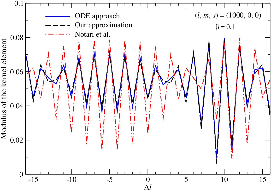
for ℓ′>ℓ\ell^{\prime}>\ell, and then use 𝒦ℓ​ℓms​(η)≈J0​(η​ℓ2−m2){}_{s}\mathcal{K}^{m}_{\ell\ell}(\eta)\approx J_{0}\left(\eta\,\sqrt{\ell^{2}-m^{2}}\right) and 𝒦ℓ′​ℓms​(η)=(−1)ℓ′−ℓ​𝒦ℓ​ℓ′ms​(η){}_{s}\mathcal{K}^{m}_{\ell^{\prime}\ell}(\eta)=(-1)^{\ell^{\prime}-\ell}{}_{s}\mathcal{K}^{m}_{\ell\ell^{\prime}}(\eta) otherwise. This is similar to the expressions in Eq. (8)-(10) given of [23], however, there the functional form was obtained from fits to the numerical results at ℓ≲700\ell\lesssim 700 rather than by analytic arguments. Our expression also works well for very large values of β\beta. This is illustrated in Fig. 2 for β=0.1\beta=0.1, ℓ=1000\ell=1000 and m=0m=0. Even for these extreme values of β\beta, our approximation reproduces the main trend and amplitude of the numerical result, while Eq. (8)-(10) of [23] become more crude 11 1 In a footnote, Notari et al [23] suggested the replacement β→β/(1−β2)1/4\beta\rightarrow\beta/(1-\beta^{2})^{1/4} to improve the convergence of their expressions. While the leading order correction β/(1−β2)1/4≃β+β3/4\beta/(1-\beta^{2})^{1/4}\simeq\beta+\beta^{3}/4 differs from η≃β−β3/3\eta\simeq\beta-\beta^{3}/3, we find that this indeed does improve the validity of the approximations provided there.. Still, the approximation Eq. (47) is valid only at Δ​ℓ/ℓ≲1\Delta\ell/\ell\lesssim 1, and since the kernel becomes wide as ℓ\ell and β\beta increase [26], the applicability of the Bessel approximation is generally limited.

We carefully checked the precision of the approximations against the results obtained with the ODE approach and found that overall the typical error is very small (≃0.1%−5%\simeq 0.1\%-5\% for β=10−3\beta=10^{-3} and ℓ≤4000\ell\leq 4000). However, even for rather small Δ​ℓ≃1\Delta\ell\simeq 1, ℓ≫1\ell\gg 1 and β≃10−3\beta\simeq 10^{-3} we occasionally find that the approximation can be off by a large amount, when the kernel value is close to zero-crossing (e.g., for β=10−3\beta=10^{-3}, ℓ≃ℓ′≃2404\ell\simeq\ell^{\prime}\simeq 2404 and m≃0m\simeq 0, which is off by a factor of ≃1.5\simeq 1.5). Also, the approximation is generally less accurate for ℓ≃m\ell\simeq m. We thus do not recommend using the expressions for real computations, also because the ODE approach already is very fast and reliable.
Refer to caption
Figure 2: Modulus of 𝒦ℓ+Δ​ℓ​ℓm0{}_{0}\mathcal{K}^{m}_{\ell+\Delta\ell\,\ell} at ℓ≃ℓ′\ell\simeq\ell^{\prime} for ℓ=1000\ell=1000, m=0m=0 and β=0.1\beta=0.1. We compare our numerical result with the approximation Eq. (47) and Eq. (8)-(10) given in [23].

VI.2 Series expansion in orders of η\eta

From Eq. (44), we can also obtain simple term-by-term approximations for the aberration kernels. Rescaling them by Nℓ′​ℓ=ηΔ​ℓ​∏k=1Δ​ℓBℓ+kmsN_{\ell^{\prime}\ell}=\eta^{\Delta\ell}\prod_{k=1}^{\Delta\ell}{}_{s}B^{m}_{\ell+k}, for ℓ′>ℓ\ell^{\prime}>\ell Eq. (44) becomes

Δ​ℓ​𝒦¯ℓ′​ℓms+η​∂η𝒦¯ℓ′​ℓms\displaystyle\Delta\ell\,{}_{s}\bar{\mathcal{K}}^{m}_{\ell^{\prime}\ell}+\eta\,\partial_{\eta}{}_{s}\bar{\mathcal{K}}^{m}_{\ell^{\prime}\ell} =𝒦¯ℓ′​ℓ+1ms−(η​Bℓms)2​𝒦¯ℓ′​ℓ−1ms,\displaystyle={}_{s}\bar{\mathcal{K}}^{m}_{\ell^{\prime}\ell+1}-(\eta{}_{s}B^{m}_{\ell})^{2}{}_{s}\bar{\mathcal{K}}^{m}_{\ell^{\prime}\ell-1},

where 𝒦¯ℓ′​ℓms=𝒦ℓ′​ℓms/Nℓ′​ℓ{}_{s}\bar{\mathcal{K}}^{m}_{\ell^{\prime}\ell}={}_{s}\mathcal{K}^{m}_{\ell^{\prime}\ell}/N_{\ell^{\prime}\ell}. Inserting the series ansatz 𝒦¯ℓ′​ℓms=∑k=0∞(−1)k​κ¯ℓ′​ℓm⁡(k)s​η2​k/(2​k+Δ​ℓ)!{}_{s}\bar{\mathcal{K}}^{m}_{\ell^{\prime}\ell}=\sum_{k=0}^{\infty}(-1)^{k}\,{}_{s}\bar{\kappa}^{m(k)}_{\ell^{\prime}\ell}\eta^{2k}/(2k+\Delta\ell)!, after collecting terms we find

κ¯ℓ′​ℓm⁡(k)s\displaystyle\,{}_{s}\bar{\kappa}^{m(k)}_{\ell^{\prime}\ell} =κ¯ℓ′​ℓ+1m⁡(k)s+(Bℓms)2​κ¯ℓ′​ℓ−1m⁡(k−1)s,\displaystyle=\,{}_{s}\bar{\kappa}^{m(k)}_{\ell^{\prime}\ell+1}+({}_{s}B^{m}_{\ell})^{2}\,{}_{s}\bar{\kappa}^{m(k-1)}_{\ell^{\prime}\ell-1}, (48)

with κ¯ℓ′​ℓm⁡(0)s=1\,{}_{s}\bar{\kappa}^{m(0)}_{\ell^{\prime}\ell}=1 and κ¯ℓ′​ℓm⁡(k)s=0\,{}_{s}\bar{\kappa}^{m(k)}_{\ell^{\prime}\ell}=0 for k<0k<0.

For ℓ=ℓ′\ell=\ell^{\prime}, we proceed similarly, finding

κ¯ℓ​ℓm⁡(k)s\displaystyle\,{}_{s}\bar{\kappa}^{m(k)}_{\ell\ell} =(Bℓ+1ms)2​κ¯ℓ+1​ℓm⁡(k−1)s+(Bℓms)2​κ¯ℓ​ℓ−1m⁡(k−1)s.\displaystyle=({}_{s}B^{m}_{\ell+1})^{2}\,{}_{s}\bar{\kappa}^{m(k-1)}_{\ell+1\ell}+({}_{s}B^{m}_{\ell})^{2}\,{}_{s}\bar{\kappa}^{m(k-1)}_{\ell\ell-1}. (49)

With κ¯ℓ′​ℓm⁡(0)s=1\,{}_{s}\bar{\kappa}^{m(0)}_{\ell^{\prime}\ell}=1, for the η2\eta^{2} correction to the diagonal term this equation directly implies

κ¯ℓ​ℓm⁡(1)s=(Bℓms)2+(Bℓ+1ms)2.\displaystyle\,{}_{s}\bar{\kappa}^{m(1)}_{\ell\ell}=({}_{s}B^{m}_{\ell})^{2}+({}_{s}B^{m}_{\ell+1})^{2}. (50)

Inserting this back into Eq. (48), we then find

κ¯ℓ′​ℓm⁡(1)s=∑k=0Δ​ℓ+1(Bℓ+kms)2.\displaystyle\,{}_{s}\bar{\kappa}^{m(1)}_{\ell^{\prime}\ell}=\sum_{k=0}^{\Delta\ell+1}({}_{s}B^{m}_{\ell+k})^{2}. (51)

for ℓ′>ℓ\ell^{\prime}>\ell. Repeating the process, we have

κ¯ℓ​ℓm⁡(2)s\displaystyle\,{}_{s}\bar{\kappa}^{m(2)}_{\ell\ell} =∑k=01∑p=02(Bℓ+kms)2​(Bℓ+k+p−1ms)2\displaystyle=\sum_{k=0}^{1}\sum_{p=0}^{2}({}_{s}B^{m}_{\ell+k})^{2}({}_{s}B^{m}_{\ell+k+p-1})^{2} (52a)
κ¯ℓ′​ℓm⁡(2)s\displaystyle\,{}_{s}\bar{\kappa}^{m(2)}_{\ell^{\prime}\ell} =∑k=01∑p=02(Bℓ′+kms)2​(Bℓ′+k+p−1ms)2\displaystyle=\sum_{k=0}^{1}\sum_{p=0}^{2}({}_{s}B^{m}_{\ell^{\prime}+k})^{2}({}_{s}B^{m}_{\ell^{\prime}+k+p-1})^{2}
+∑k=0Δ​ℓ−1∑p=0Δ​ℓ+2−k(Bℓ+kms)2(Bℓ−1+k+pms)2\displaystyle\qquad+\sum_{k=0}^{\Delta\ell-1}\sum_{p=0}^{\Delta\ell+2-k}({}_{s}B^{m}_{\ell+k})^{2}({}_{s}B^{m}_{\ell-1+k+p})^{2} (52b)

for the η4\eta^{4} correction to the kernels. Higher order terms can be obtained in a similar way, but generally it is simpler to just evaluate the recursions Eq. (48) and (49) in an alternating manner, so that we do not give additional explicit expressions here. We note that the form of the recursions also explicitly shows that the kernel for d=1d=1 does not depend on the sign of the spin weight and hence directly proves 𝒦ℓ′​ℓms​(η)≡𝒦ℓ′​ℓm−s​(η){}_{s}\mathcal{K}^{m}_{\ell^{\prime}\ell}(\eta)\equiv{}_{-s}\mathcal{K}^{m}_{\ell^{\prime}\ell}(\eta) required to avoid EE/BB-mode mixing (Sect. IV).

From Eq. (51), we can also understand why the approximation Eq. (47) is only expected to work for Δ​ℓ≪ℓ\Delta\ell\ll\ell. The first two terms in the Taylor series are

𝒦ℓ′​ℓms​(η)\displaystyle{}_{s}\mathcal{K}^{m}_{\ell^{\prime}\ell}(\eta) ≈ηΔ​ℓ​∏k=1Δ​ℓBℓ+kms​[1Δ​ℓ!−∑k=0Δ​ℓ+1(Bℓ+kms​η)2(Δ​ℓ+2)!]\displaystyle\approx\eta^{\Delta\ell}\prod_{k=1}^{\Delta\ell}{}_{s}B^{m}_{\ell+k}\left[\frac{1}{\Delta\ell!}-\frac{\sum_{k=0}^{\Delta\ell+1}({}_{s}B^{m}_{\ell+k}\eta)^{2}}{(\Delta\ell+2)!}\right]
≈(2​Bℓms​η)Δ​ℓ2Δ​ℓ​Δ​ℓ!​[1−(2​Bℓms​η)24​(Δ​ℓ+1)]≈JΔ​ℓ​(2​Bℓms​η),\displaystyle\approx\frac{(2{}_{s}B^{m}_{\ell}\,\eta)^{\Delta\ell}}{2^{\Delta\ell}\Delta\ell!}\left[1-\frac{(2{}_{s}B^{m}_{\ell}\eta)^{2}}{4(\Delta\ell+1)}\right]\approx J_{\Delta\ell}(2{}_{s}B^{m}_{\ell}\,\eta),

which only for Δ​ℓ≪ℓ\Delta\ell\ll\ell and κ¯ℓ′​ℓm⁡(1)s≈(Δ​ℓ+2)​(Bℓms)2\,{}_{s}\bar{\kappa}^{m(1)}_{\ell^{\prime}\ell}\approx(\Delta\ell+2)({}_{s}B^{m}_{\ell})^{2} can be identified with the Bessel approximation given above.

VII Conclusion

In this paper, we found a novel matrix representation for the harmonic-space aberration kernels. Several useful and exact relations are then derived by utilizing the commutation relations for the rotation and boost operators. CMB observables with Doppler weight d=1d=1 (e.g., the polarization-averaged temperature and the temperature-weighted Stokes parameters), have the simplest transformation properties. We showed that the d=1d=1 kernels are the matrix elements of a boost operator, parameterized by the additive rapidity parameter, between two spherical harmonic base states.

The unitarity of the boost operator leads to power conservation laws under aberration, which are valid for d=1d=1. The Lorentz algebra, satisfied by generators of rotations (both space-fixed and body-fixed) and boosts, lead to recursion relations that raise or lower the spherical harmonic quantum numbers ℓ\ell and mm, or the spin weight ss by one unit. These provide useful identities in analytical calculations. Applying these recursions repeatedly, starting from known kernels of the lowest ℓ\ell, |m||m| and |s||s| as suitable boundary conditions, yields kernels with arbitrary ℓ\ell, mm and ss. Based on this, the new recursion scheme developed here greatly simplifies previous recursive algorithms at both conceptual and technical levels. It also provides exact values for the aberration kernels to benchmark the accuracy of existing fitting formula.

We proved that aberration does not mix up EE and BB modes for d=1d=1 polarization observables to all orders in β\beta. We argued that for perfect blackbody spectra, d=1d=1 kernels are the relevant ones for the study of CMB aberration, independent of experimental details. In the presence of spectrum distortions and foreground emissions, the correct way to account for the aberration effect deserves further consideration. For general purposes, we provided recipes to compute aberration kernels of Doppler weight d≠1d\neq 1, relevant for boosting, e.g., the specific intensity or the frequency-integrated intensity. Those have been shown to be related to the d=1d=1 kernels via dd-raising/lowering recursions.

Another major result derived from the matrix-element representation is the flow of the d=1d=1 aberration kernels with the rapidity parameter η\eta. This leads to coupled ODEs for a set of aberration kernels that in practice can be effectively truncated. The ODE approach is very advantageous because the initial conditions needed, i.e. the kernels for η=0\eta=0, are in all cases trivial, and therefore extremely straightforward to set up. Utilizing standard recipes, the ODE approach can improve upon the recursive approach by a factor ∼25\sim 25 in terms of computational speed, for moderate values of β∼10−3\beta\sim 10^{-3}. Parallelization is straightforward in the ODE approach, pushing the computation of the aberration kernel to a few seconds.

In the limit of large ℓ\ell, we find simple asymptotic approximations for the kernel elements from the differential equation system (Sec. VI.1). While similar to the expressions given earlier by [23], we obtain our approximations with purely analytic arguments. Our approximation generally work very well (≃0.1%−5%\simeq 0.1\%-5\% for β=10−3\beta=10^{-3} and ℓ≤4000\ell\leq 4000), however, when comparing with our ODE approach we find several cases for which the approximation is very far off. For Δ​ℓ/ℓ≪1\Delta\ell/\ell\ll 1, our expressions also capture the main dependence of the kernel even for β≃0.1\beta\simeq 0.1; however, since the kernel becomes very wide once ℓ≫1/β\ell\gg 1/\beta, the approximation still has limited applicability. We thus do not recommend using the expression for real computations, also because the ODE approach already is very fast and reliable.

Finally, we emphasize that most of the analytical results obtained in this paper apply to all angular scales ℓ\ell, arbitrary spin weight ss and Doppler weight dd, being fully non-linear in β\beta. Therefore, our formalism might find applications in other studies, where anisotropic radiation seen in a (relativistically) boosted reference frame is involved. One example is the scattering of diffuse photon backgrounds by fast-moving charged particles within the jets of active galactic nuclei [32, 31, 33].

Acknowledgements.
The authors thank Donghui Jeong, Marc Kamionkowski and Jared Kaplan for useful discussions. We also thank Miguel Quartin and Alessio Notari for comments on the first draft of the paper. This work was supported by DoE SC-0008108 and NASA NNX12AE86G.

Appendix A Deriving the integral forms for the aberration kernels

In the literature, different approaches of deriving the aberration kernels for both temperature and polarization have been presented (see e.g. [10, 34]). All are essentially based on how the photon’s four-momentum and polarization tensor transform under a Lorentz boost of the reference frame. Here we adopt the covariant formalism of Ref. [35].

The photon phase space density needs to be described by a Lorentz tensor Fμ​νF_{\mu\nu} (not to be confused with the usual electromagnetic field-strength tensor), for there are two distinct polarization states. The observer’s motion defines a unique time-like unit vector eoμe^{\mu}_{o}, and its line of sight direction (opposite to the direction of propagation) defines a space-like unit vector nμn^{\mu} orthogonal to eoμe^{\mu}_{o}. The symmetric screen-projection tensor can be defined as

Sμ(eo,n)ν=gμ+νeoμeo,ν−nμnν,\displaystyle S^{\mu}{}_{\nu}(e_{o},n)=g^{\mu}{}_{\nu}+e^{\mu}_{o}e_{o,\nu}-n^{\mu}n_{\nu}, (53)

where gμ​νg_{\mu\nu} is the flat Minkowski metric. A gauge-invariant phase space density fμ​νf_{\mu\nu} can be then obtained by screen-projection, i.e. fμ​ν=Sρ​Sσμ​Fρ​σνf_{\mu\nu}=S^{\rho}{}_{\mu}S^{\sigma}{}_{\nu}F_{\rho\sigma}. Neglecting circular polarization, which is irrelevant for the CMB, the gauge-invariant fμ​νf_{\mu\nu} can be decomposed into

fμ​ν​(E,𝒏^)=12​N​(E,𝒏^)​Sμ​ν+Pμ​ν​(E,𝒏^),\displaystyle f_{\mu\nu}(E,\boldsymbol{\hat{n}})=\frac{1}{2}N(E,\boldsymbol{\hat{n}})S_{\mu\nu}+P_{\mu\nu}(E,\boldsymbol{\hat{n}}), (54)

where N=gμ​ν​fμ​νN=g^{\mu\nu}f_{\mu\nu} is the occupation number including both polarization states, and the symmetric trace-free Pμ​νP_{\mu\nu} encodes the difference between the two linear polarizations. Note that photon phase space density is a function of the measured photon 4-momentum pμ=E⁡(eoμ−nμ)p^{\mu}=E(e^{\mu}_{o}-n^{\mu}), or equivalently a function of the measured energy EE and the measured line of sight direction nμn^{\mu}. We have made this dependence manifest.

Next we need to know how fμ​νf_{\mu\nu} transforms under a Lorentz boost. Note that due to the screen-projection procedure it transforms differently from how a usual Lorentz tensor does. To derive the correct transformation rule, let us consider another observer,

eo′μ=γ⁡(eoμ+vμ),γ=1/1−vμ​vμ=1/1−β2,eoμ​vμ=0,\displaystyle e^{\mu}_{o^{\prime}}=\gamma(e^{\mu}_{o}+v^{\mu}),\hskip 18.49988pt\gamma=1/\sqrt{1-v^{\mu}v_{\mu}}=1/\sqrt{1-\beta^{2}},\hskip 18.49988pte^{\mu}_{o}v_{\mu}=0, (55)

which has velocity vμv^{\mu} relative to the original observer. The new observer will measure screen-projected phase space density fμ​ν′=S′ρ​S′σμ​Fρ​σνf_{\mu\nu}^{\prime}=S^{\prime\rho}{}_{\mu}S^{\prime\sigma}{}_{\nu}F_{\rho\sigma}, where S′μ=νS′μ(eo′,n′)νS^{\prime\mu}{}_{\nu}=S^{\prime\mu}{}_{\nu}(e_{o^{\prime}},n^{\prime}) is the boosted screen-projection tensor constructed from the new time direction eo′μe^{\mu}_{o^{\prime}} and the aberrated line of sight direction

n′μ=−eoμ−nμγ⁡(1+nν​vν)+γ⁡(eoμ+vμ).\displaystyle n^{\prime\mu}=-\frac{e^{\mu}_{o}-n^{\mu}}{\gamma(1+n^{\nu}v_{\nu})}+\gamma(e^{\mu}_{o}+v^{\mu}). (56)

Besides, the photon energy is shifted to

E=E′​γ​(1−n′μ​vμ).\displaystyle E=E^{\prime}\gamma(1-n^{\prime\mu}v_{\mu}). (57)

A nice property is that S′μνS^{\prime\mu}{}_{\nu} can be obtained from SμνS^{\mu}{}_{\nu} simply through further screen-projections S′μν=S′μρS′σνSρσS^{\prime\mu}{}_{\nu}=S^{\prime\mu}{}_{\rho}S^{\prime\sigma}{}_{\nu}S^{\rho}{}_{\sigma}. After simple algebra this leads to the transformation of NN and Pμ​νP_{\mu\nu},

N′​(E′,𝒏^′)=N⁡(E,𝒏^),Pμ​ν′​(E′,𝒏^′)=S′ρ​S′σμ​Pρ​σν​(E,𝒏^).\displaystyle N^{\prime}(E^{\prime},\boldsymbol{\hat{n}}^{\prime})=N(E,\boldsymbol{\hat{n}}),\hskip 18.49988ptP^{\prime}_{\mu\nu}(E^{\prime},\boldsymbol{\hat{n}}^{\prime})=S^{\prime\rho}{}_{\mu}S^{\prime\sigma}{}_{\nu}P_{\rho\sigma}(E,\boldsymbol{\hat{n}}). (58)

A.1 Temperature kernels

For a blackbody spectrum, we have N⁡(E,nμ)=2/(eE/T⁡(𝒏^)−1)N(E,n^{\mu})=2/(e^{E/T(\boldsymbol{\hat{n}})}-1). Under a Lorentz boost the blackbody shape is preserved. Eq. (58) then implies that E′/T′​(𝒏^′)=E/T⁡(𝒏^)E^{\prime}/T^{\prime}(\boldsymbol{\hat{n}}^{\prime})=E/T(\boldsymbol{\hat{n}}). Using Eq. (57), we thus immediately confirm T′(𝒏^′)=T(𝒏^)/[γ(1−βcosθ′)]T^{\prime}(\boldsymbol{\hat{n}}^{\prime})=T(\boldsymbol{\hat{n}})/[\gamma(1-\beta\cos\theta^{\prime})]. We can then compute the boosted temperature multipole coefficients,

al′​m′′T=∫d2​𝒏^′​Yl′​m′∗​(𝒏^′)​T′​(𝒏^′)=∫d2​𝒏^′​Yl′​m′∗​(𝒏^′)​T​(n)γ⁡(1−n′μ​vμ)=∑l​mal​mT​∫d2​𝒏^′​Yl′​m′∗​(𝒏^′)​Yl​m​(𝒏^)γ⁡(1−n′μ​vμ).\displaystyle a^{\prime T}_{l^{\prime}m^{\prime}}=\int{\rm d}^{2}\boldsymbol{\hat{n}}^{\prime}Y^{*}_{l^{\prime}m^{\prime}}(\boldsymbol{\hat{n}}^{\prime})T^{\prime}(\boldsymbol{\hat{n}}^{\prime})=\int{\rm d}^{2}\boldsymbol{\hat{n}}^{\prime}\frac{Y^{*}_{l^{\prime}m^{\prime}}(\boldsymbol{\hat{n}}^{\prime})T(n)}{\gamma\left(1-n^{\prime\mu}v_{\mu}\right)}=\sum_{lm}a^{T}_{lm}\int{\rm d}^{2}\boldsymbol{\hat{n}}^{\prime}\frac{Y^{*}_{l^{\prime}m^{\prime}}(\boldsymbol{\hat{n}}^{\prime})Y_{lm}(\boldsymbol{\hat{n}})}{\gamma\left(1-n^{\prime\mu}v_{\mu}\right)}. (59)

Given that n′μvμ=βcosθ′n^{\prime\mu}v_{\mu}=\beta\cos\theta^{\prime} and that for boosts along the zz-direction the azimuthal integral gives δm​m′\delta_{mm^{\prime}}, together with the definition Eq. (3) for the aberration kernel, we confirm Eq. (4) for s=0s=0.

A.2 Polarization kernels

We use the notations and properties of tensor spherical harmonics as developed in Ref. [28]. We consider the temperature-weighted polarization tensor

𝒫μ​ν​(𝒏^)≡T⁡(𝒏^)​Pμ​ν​(E,𝒏^)/N⁡(E,𝒏^).\displaystyle\mathcal{P}_{\mu\nu}(\boldsymbol{\hat{n}})\equiv T(\boldsymbol{\hat{n}})P_{\mu\nu}(E,\boldsymbol{\hat{n}})/N(E,\boldsymbol{\hat{n}}). (60)

Assuming no deviation from a blackbody spectrum, the photon energy EE cancels out in 𝒫μ​ν\mathcal{P}_{\mu\nu}.

Orthogonal to eoμe^{\mu}_{o} and nμn^{\mu}, we can choose two space-like unit vectors eaμ​(𝒏^)e^{\mu}_{a}(\boldsymbol{\hat{n}}) with a=1,2a=1,2, which is unaffected by screen projection eaμ(𝒏^)Sν(𝒏^)μ=eaν(𝒏^)e^{\mu}_{a}(\boldsymbol{\hat{n}})S^{\nu}{}_{\mu}(\boldsymbol{\hat{n}})=e^{\nu}_{a}(\boldsymbol{\hat{n}}). Since 𝒫μ​ν\mathcal{P}_{\mu\nu} is screen-projected, we can construct the two-by-two transverse tensor

𝒫a​b​(𝒏^)=eaμ​(𝒏^)​ebν​(𝒏^)​𝒫μ​ν​(𝒏^).\displaystyle\mathcal{P}_{ab}(\boldsymbol{\hat{n}})=e^{\mu}_{a}(\boldsymbol{\hat{n}})e^{\nu}_{b}(\boldsymbol{\hat{n}})\mathcal{P}_{\mu\nu}(\boldsymbol{\hat{n}}). (61)

We now compute the transformation of 𝒫a​b\mathcal{P}_{ab}

𝒫a′​b′′​(𝒏^′)\displaystyle\mathcal{P}^{\prime}_{a^{\prime}b^{\prime}}(\boldsymbol{\hat{n}}^{\prime}) =\displaystyle= ea′′μ(𝒏^′)eb′′ν(n^′)𝒫μ​ν′(𝒏^′)=ea′′μ(𝒏^′)eb′′ν(𝒏^′)Sμ′(n^′)ρSν′(𝒏^′)σT′​(𝒏^′)T⁡(𝒏^)𝒫ρ​σ(𝒏^)\displaystyle e^{\prime\mu}_{a^{\prime}}(\boldsymbol{\hat{n}}^{\prime})e^{\prime\nu}_{b^{\prime}}(\hat{n}^{\prime})\mathcal{P}^{\prime}_{\mu\nu}(\boldsymbol{\hat{n}}^{\prime})=e^{\prime\mu}_{a^{\prime}}(\boldsymbol{\hat{n}}^{\prime})e^{\prime\nu}_{b^{\prime}}(\boldsymbol{\hat{n}}^{\prime})S^{\prime}_{\mu}{}^{\rho}(\hat{n}^{\prime})S^{\prime}_{\nu}{}^{\sigma}(\boldsymbol{\hat{n}}^{\prime})\frac{T^{\prime}(\boldsymbol{\hat{n}}^{\prime})}{T(\boldsymbol{\hat{n}})}\mathcal{P}_{\rho\sigma}(\boldsymbol{\hat{n}}) (62)
=\displaystyle= T′​(𝒏^′)T⁡(𝒏^)​ea′′ρ​(𝒏^′)​eb′′σ​(𝒏^′)​𝒫ρ​σ​(𝒏^)=T′​(𝒏^′)T⁡(𝒏^)​ea′′ρ​(𝒏^′)​eb′′σ​(𝒏^′)​ea,ρ​(𝒏^)​eb,σ​(𝒏^)​𝒫a​b​(𝒏^).\displaystyle\frac{T^{\prime}(\boldsymbol{\hat{n}}^{\prime})}{T(\boldsymbol{\hat{n}})}e^{\prime\rho}_{a^{\prime}}(\boldsymbol{\hat{n}}^{\prime})e^{\prime\sigma}_{b^{\prime}}(\boldsymbol{\hat{n}}^{\prime})\mathcal{P}_{\rho\sigma}(\boldsymbol{\hat{n}})=\frac{T^{\prime}(\boldsymbol{\hat{n}}^{\prime})}{T(\boldsymbol{\hat{n}})}e^{\prime\rho}_{a^{\prime}}(\boldsymbol{\hat{n}}^{\prime})e^{\prime\sigma}_{b^{\prime}}(\boldsymbol{\hat{n}}^{\prime})e_{a,\rho}(\boldsymbol{\hat{n}})e_{b,\sigma}(\boldsymbol{\hat{n}})\mathcal{P}_{ab}(\boldsymbol{\hat{n}}).

The spherical harmonic expansion for the polarization tensor reads

𝒫a​b​(𝒏^)=∑ℓ​m∑s=±2aℓ​ms​Y(ℓ​m)​a​bs​(𝒏^),\displaystyle\mathcal{P}_{ab}(\boldsymbol{\hat{n}})=\sum_{\ell m}\sum_{s=\pm 2}a^{s}_{\ell m}Y^{s}_{(\ell m)ab}(\boldsymbol{\hat{n}}), (63)

and similar in the boosted frame. Here Y(ℓ​m)​a​b±2​(𝒏^)Y^{\pm 2}_{(\ell m)ab}(\boldsymbol{\hat{n}}) are the tensor spherical harmonics of definite helicity [28]. A derivation parallel to that for temperature then gives the tranformation of the multipole coefficients,

aℓ′​m′′s′=∑ℓ​m∑s=±2aℓ′​m′s​∫d2​𝒏^′​[Y(l′​m′)​a′​b′s′​(𝒏^′)]∗​Y(l​m)​a​bs​(𝒏^)γ⁡(1−n′ν​vν)​ea′′ρ​(𝒏^′)​eb′′σ​(𝒏^′)​ea,ρ​(𝒏^)​eb,σ​(𝒏^).\displaystyle a^{\prime s^{\prime}}_{\ell^{\prime}m^{\prime}}=\sum_{\ell m}\sum_{s=\pm 2}a^{s}_{\ell^{\prime}m^{\prime}}\int{\rm d}^{2}\boldsymbol{\hat{n}}^{\prime}\frac{[Y^{s^{\prime}}_{(l^{\prime}m^{\prime})a^{\prime}b^{\prime}}(\boldsymbol{\hat{n}}^{\prime})]^{*}Y^{s}_{(lm)ab}(\boldsymbol{\hat{n}})}{\gamma\left(1-n^{\prime\nu}v_{\nu}\right)}e^{\prime\rho}_{a^{\prime}}(\boldsymbol{\hat{n}}^{\prime})e^{\prime\sigma}_{b^{\prime}}(\boldsymbol{\hat{n}}^{\prime})e_{a,\rho}(\boldsymbol{\hat{n}})e_{b,\sigma}(\boldsymbol{\hat{n}}). (64)

We can relate the tensor spherical harmonics to the spin-weighted harmonics Y(ℓ​m)​a​b±2​(𝒏^)=Y(ℓ​m)∓2​(𝒏^)​ε∓2,a​b​(𝒏^)Y^{\pm 2}_{(\ell m)ab}(\boldsymbol{\hat{n}})=\,{}_{\mp 2}Y_{(\ell m)}(\boldsymbol{\hat{n}})\varepsilon_{\mp 2,ab}(\boldsymbol{\hat{n}}) [28], with ε∓2,a​b​(𝒏^)\varepsilon_{\mp 2,ab}(\boldsymbol{\hat{n}}) being the usual spin-2 base tensors on the sphere. Then we find

aℓ′​m′′s′=∑ℓ​m∑s=±2aℓ′​m′s​∫d2​𝒏^′​[Y(ℓ′​m′)−s′​(𝒏^′)]∗​Y(ℓ​m)−s​(𝒏^)γ⁡(1−n′ν​vν)​[ε−s′′μ​ν​(𝒏^′)]∗​ε−s,μ​ν​(𝒏^),\displaystyle a^{\prime s^{\prime}}_{\ell^{\prime}m^{\prime}}=\sum_{\ell m}\sum_{s=\pm 2}a^{s}_{\ell^{\prime}m^{\prime}}\int{\rm d}^{2}\boldsymbol{\hat{n}}^{\prime}\frac{[{}_{-s^{\prime}}Y_{(\ell^{\prime}m^{\prime})}(\boldsymbol{\hat{n}}^{\prime})]^{*}{}_{-s}Y_{(\ell m)}(\boldsymbol{\hat{n}})}{\gamma\left(1-n^{\prime\nu}v_{\nu}\right)}[\varepsilon^{\prime\mu\nu}_{-s^{\prime}}(\boldsymbol{\hat{n}}^{\prime})]^{*}\varepsilon_{-s,\mu\nu}(\boldsymbol{\hat{n}}), (65)

with ε−sμ​ν​(𝒏^)=ε−s,a​b​(𝒏^)​eaμ​(𝒏^)​ebν​(𝒏^)\varepsilon^{\mu\nu}_{-s}(\boldsymbol{\hat{n}})=\varepsilon_{-s,ab}(\boldsymbol{\hat{n}})e^{\mu}_{a}(\boldsymbol{\hat{n}})e^{\nu}_{b}(\boldsymbol{\hat{n}}), and similar definition for ε−s′′μ​ν​(𝒏^′)\varepsilon^{\prime\mu\nu}_{-s^{\prime}}(\boldsymbol{\hat{n}}^{\prime}) as measured in the boosted frame. By explicitly constructing the transverse base vectors eaμ​(𝒏^)e^{\mu}_{a}(\boldsymbol{\hat{n}}), and similarly for ea′μ​(𝒏^′)e^{\prime\mu}_{a}(\boldsymbol{\hat{n}}^{\prime}) in the boosted frame, one find simple results,

[ε±2′μ​ν​(𝒏^′)]∗​ε±2,μ​ν​(𝒏^)=1,[ε±2′μ​ν​(𝒏^′)]∗​ε∓2,μ​ν​(𝒏^)=0.\displaystyle[\varepsilon^{\prime\mu\nu}_{\pm 2}(\boldsymbol{\hat{n}}^{\prime})]^{*}\varepsilon_{\pm 2,\mu\nu}(\boldsymbol{\hat{n}})=1,\hskip 18.49988pt[\varepsilon^{\prime\mu\nu}_{\pm 2}(\boldsymbol{\hat{n}}^{\prime})]^{*}\varepsilon_{\mp 2,\mu\nu}(\boldsymbol{\hat{n}})=0. (66)

Eq. (65) then simplifies to

aℓ′​m′′±2=∑ℓ​maℓ′​m′±2​∫d2​𝒏^′​[Y(ℓ′​m′)∓2​(𝒏^′)]∗​Y(ℓ​m)∓2​(𝒏^)γ⁡(1−n′ν​vν).\displaystyle a^{\prime\pm 2}_{\ell^{\prime}m^{\prime}}=\sum_{\ell m}a^{\pm 2}_{\ell^{\prime}m^{\prime}}\int{\rm d}^{2}\boldsymbol{\hat{n}}^{\prime}\frac{[{}_{\mp 2}Y_{(\ell^{\prime}m^{\prime})}(\boldsymbol{\hat{n}}^{\prime})]^{*}{}_{\mp 2}Y_{(\ell m)}(\boldsymbol{\hat{n}})}{\gamma\left(1-n^{\prime\nu}v_{\nu}\right)}. (67)

Again, given that n′μvμ=βcosθ′n^{\prime\mu}v_{\mu}=\beta\cos\theta^{\prime} and that the integral gives δm​m′\delta_{mm^{\prime}}, together with the definition Eq. (3) for the aberration kernel, we obtain exactly Eq. (4) for s=±2s=\pm 2.

Appendix B Proof of general kernel properties

Here, we briefly prove the general kernel properties, Eq. (8). We start with 𝒦ℓ′​ℓ−m−sd​(β)=𝒦ℓ′​ℓmsd​(β)\,{}^{d}_{-s}\mathcal{K}^{-m}_{\ell^{\prime}\ell}(\beta)=\,{}^{d}_{s}\mathcal{K}^{m}_{\ell^{\prime}\ell}(\beta), which is the simplest to show. From Eq. (5), with Yℓ′−m−s​(𝒏^′)=(−1)s+m​[Yℓ′​ms​(𝒏^′)]∗{}_{-s}Y_{\ell^{\prime}-m}(\boldsymbol{\hat{n}}^{\prime})=(-1)^{s+m}[{}_{s}Y_{\ell^{\prime}m}(\boldsymbol{\hat{n}}^{\prime})]^{*} we have

𝒦ℓ′​ℓ−m−sd​(β)=∫d2​𝒏^′​[Yℓ′−ms​(𝒏^′)]∗​Yℓ−ms​(𝒏^)[γ(1−βcosθ′)]d=∫d2​𝒏^′​Yℓ′​m−s​(𝒏^′)​[Yℓ​m−s​(𝒏^)]∗[γ(1−βcosθ′)]d=[𝒦ℓ′​ℓmsd​(β)]∗≡𝒦ℓ′​ℓmsd​(β),\displaystyle\,{}^{d}_{-s}\mathcal{K}^{-m}_{\ell^{\prime}\ell}(\beta)=\int{\rm d}^{2}\boldsymbol{\hat{n}}^{\prime}\frac{[{}_{s}Y_{\ell^{\prime}-m}(\boldsymbol{\hat{n}}^{\prime})]^{*}\,{}_{s}Y_{\ell-m}(\boldsymbol{\hat{n}})}{[\gamma(1-\beta\cos\theta^{\prime})]^{d}}=\int{\rm d}^{2}\boldsymbol{\hat{n}}^{\prime}\frac{{}_{-s}Y_{\ell^{\prime}m}(\boldsymbol{\hat{n}}^{\prime})\,[{}_{-s}Y_{\ell m}(\boldsymbol{\hat{n}})]^{*}}{[\gamma(1-\beta\cos\theta^{\prime})]^{d}}=[\,{}^{d}_{s}\mathcal{K}^{m}_{\ell^{\prime}\ell}(\beta)]^{\ast}\equiv\,{}^{d}_{s}\mathcal{K}^{m}_{\ell^{\prime}\ell}(\beta), (68)

which was our statement. Next we prove 𝒦ℓ′​ℓmsd​(−β)=(−1)ℓ+ℓ′​𝒦ℓ′​ℓm−sd​(β)\,{}^{d}_{s}\mathcal{K}^{m}_{\ell^{\prime}\ell}(-\beta)=(-1)^{\ell+\ell^{\prime}}\,{}^{d}_{-s}\mathcal{K}^{m}_{\ell^{\prime}\ell}(\beta). Imagine we perform a transformation θ→π−θ\theta\rightarrow\pi-\theta, ϕ→ϕ+π\phi\rightarrow\phi+\pi and β→−β\beta\rightarrow-\beta. Then this also means θ′→π−θ′\theta^{\prime}\rightarrow\pi-\theta^{\prime} and ϕ′→ϕ′+π\phi^{\prime}\rightarrow\phi^{\prime}+\pi, so that the kernel returns to its initial state. Using the property of spin-weighted harmonics

Yℓ​ms​(π−θ,ϕ+π)=(−1)ℓ​Yℓ​m−s​(θ,ϕ),\displaystyle{}_{s}Y_{\ell m}\left(\pi-\theta,\phi+\pi\right)=(-1)^{\ell}{}_{-s}Y_{\ell m}(\theta,\phi), (69)

from Eq. (5) we can directly infer 𝒦ℓ′​ℓmsd​(−β)=(−1)ℓ+ℓ′​𝒦ℓ′​ℓm−sd​(β)\,{}^{d}_{s}\mathcal{K}^{m}_{\ell^{\prime}\ell}(-\beta)=(-1)^{\ell+\ell^{\prime}}\,\,{}^{d}_{-s}\mathcal{K}^{m}_{\ell^{\prime}\ell}(\beta). This is a symmetry of the kernels for general dd.

Finally, we prove 𝒦ℓ​ℓ′msd​(β)=(−1)ℓ+ℓ′​𝒦ℓ′​ℓm−s2−d​(β)\,{}^{d}_{s}\mathcal{K}^{m}_{\ell\ell^{\prime}}(\beta)=(-1)^{\ell+\ell^{\prime}}\,{}^{2-d}_{-s}\mathcal{K}^{m}_{\ell^{\prime}\ell}(\beta), for which we need the identities, dcosθ′/(1−βcosθ′)=dcosθ/(1+βcosθ){\rm d}\cos\theta^{\prime}/(1-\beta\cos\theta^{\prime})={\rm d}\cos\theta/(1+\beta\cos\theta), d​ϕ′=d​ϕ{\rm d}\phi^{\prime}={\rm d}\phi and 1=γ2(1+βcosθ)(1−βcosθ′)1=\gamma^{2}(1+\beta\cos\theta)(1-\beta\cos\theta^{\prime}):

𝒦ℓ′​ℓmsd​(β)\displaystyle\,{}^{d}_{s}\mathcal{K}^{m}_{\ell^{\prime}\ell}(\beta) =∫dϕ′dcosθ′[Yℓ′​m−s​(𝒏^′)]∗​Yℓ​m−s​(𝒏^)[γ(1−βcosθ′)]d=∫dϕdcosθ[Yℓ′​m−s​(𝒏^′)]∗​Yℓ​m−s​(𝒏^)γd(1−βcosθ′)d−1(1+βcosθ)\displaystyle=\int{\rm d}\phi^{\prime}\,{\rm d}\cos\theta^{\prime}\frac{[{}_{-s}Y_{\ell^{\prime}m}(\boldsymbol{\hat{n}}^{\prime})]^{*}\,{}_{-s}Y_{\ell m}(\boldsymbol{\hat{n}})}{[\gamma(1-\beta\cos\theta^{\prime})]^{d}}=\int{\rm d}\phi\,{\rm d}\cos\theta\frac{[{}_{-s}Y_{\ell^{\prime}m}(\boldsymbol{\hat{n}}^{\prime})]^{*}\,{}_{-s}Y_{\ell m}(\boldsymbol{\hat{n}})}{\gamma^{d}\,(1-\beta\cos\theta^{\prime})^{d-1}(1+\beta\cos\theta)}
=∫d​ϕ​d​cos⁡θ​γ2​(d−1)​(1+β​cos⁡θ)d−1​[Yℓ′​m−s​(𝒏^′)]∗​Yℓ​m−s​(𝒏^)γd​(1+β​cos⁡θ)=∫d​ϕ​d​cos⁡θ​[Yℓ′​m−s​(𝒏^′)]∗​Yℓ​m−s​(𝒏^)[γ⁡(1+β​cos⁡θ)]2−d\displaystyle=\int{\rm d}\phi\,{\rm d}\cos\theta\frac{\gamma^{2(d-1)}(1+\beta\cos\theta)^{d-1}[{}_{-s}Y_{\ell^{\prime}m}(\boldsymbol{\hat{n}}^{\prime})]^{*}\,{}_{-s}Y_{\ell m}(\boldsymbol{\hat{n}})}{\gamma^{d}(1+\beta\cos\theta)}=\int{\rm d}\phi\,{\rm d}\cos\theta\frac{[{}_{-s}Y_{\ell^{\prime}m}(\boldsymbol{\hat{n}}^{\prime})]^{*}\,{}_{-s}Y_{\ell m}(\boldsymbol{\hat{n}})}{[\gamma(1+\beta\cos\theta)]^{2-d}}
=[𝒦ℓ​ℓ′ms2−d​(−β)]∗≡𝒦ℓ​ℓ′ms2−d​(−β)\displaystyle=[\,{}^{2-d}_{s}\mathcal{K}^{m}_{\ell\ell^{\prime}}(-\beta)]^{\ast}\equiv\,{}^{2-d}_{s}\mathcal{K}^{m}_{\ell\ell^{\prime}}(-\beta) (70)

from which our statement follows after using 𝒦ℓ′​ℓmsd​(−β)=(−1)ℓ+ℓ′​𝒦ℓ′​ℓm−sd​(β)\,{}^{d}_{s}\mathcal{K}^{m}_{\ell^{\prime}\ell}(-\beta)=(-1)^{\ell+\ell^{\prime}}\,\,{}^{d}_{-s}\mathcal{K}^{m}_{\ell^{\prime}\ell}(\beta).

Appendix C Acting Y^z\hat{Y}_{z} on base states

To derive Eq. (24), we start with the following identities for spin-weighted harmonics [36, 10]

μ​Yℓ​ms​(𝒏^)\displaystyle\mu\,{}_{s}Y_{\ell m}(\boldsymbol{\hat{n}}) =\displaystyle= Cℓ+1msYℓ+1​ms(𝒏^)−s​mℓ⁡(ℓ+1)Yℓ​ms(𝒏^)+sCℓmYℓ−1​ms(𝒏^),\,{}_{s}C^{m}_{\ell+1}\,{}_{s}Y_{\ell+1\,m}(\boldsymbol{\hat{n}})-\frac{sm}{\ell(\ell+1)}\,{}_{s}Y_{\ell m}(\boldsymbol{\hat{n}})+\,_{s}C^{m}_{\ell}\,{}_{s}Y_{\ell-1\,m}(\boldsymbol{\hat{n}}), (71a)
1−μ2​∂θYℓ​ms​(𝒏^)\displaystyle\sqrt{1-\mu^{2}}\,\partial_{\theta}\,{}_{s}Y_{\ell m}(\boldsymbol{\hat{n}}) =\displaystyle= ℓs​Cℓ+1m​Yℓ+1​ms​(𝒏^)+s​mℓ⁡(ℓ+1)​Yℓ​ms​(𝒏^)−(ℓ+1)s​Cℓm​Yℓ−1​ms​(𝒏^).\displaystyle\ell\,_{s}C^{m}_{\ell+1}\,{}_{s}Y_{\ell+1\,m}(\boldsymbol{\hat{n}})+\frac{sm}{\ell(\ell+1)}\,{}_{s}Y_{\ell m}(\boldsymbol{\hat{n}})-(\ell+1)\,_{s}C^{m}_{\ell}\,{}_{s}Y_{\ell-1\,m}(\boldsymbol{\hat{n}}). (71b)

where μ=cos⁡θ\mu=\cos\theta and sCmℓ=sBmℓ/ℓ≡(ℓ2−m2)​(ℓ2−s2)/(4​ℓ2−1)/ℓ\,{}_{s}C^{m}_{\ell}=\,_{s}B^{m}_{\ell}/\ell\equiv\sqrt{(\ell^{2}-m^{2})(\ell^{2}-s^{2})/(4\ell^{2}-1)}/\ell. From Eq. (15), we see that Y^z\hat{Y}_{z} is just the sum of cos⁡θ\cos\theta and sinθ∂θ\sin\theta\partial_{\theta}. When acting on |sℓm⟩\left|\left.s\ell m\right.\right\rangle, or explicitly D~s​mℓ\tilde{D}^{\ell}_{sm}, we just have to put back the ψ\psi-independence ei​s​ψ{\rm e}^{is\psi}. The terms proportional to |sℓm⟩\left|\left.s\ell m\right.\right\rangle on the right hand side cancel, and we obtain Eq. (24).

Appendix D Independence of the kernel on the sign of the spin weight ss for d=1d=1

For convenience, we regard aberration kernels as functions of the rapidity η\eta. Since β→−β\beta\rightarrow-\beta implies η→−η\eta\rightarrow-\eta, from Eq. (8) we also have 𝒦ℓ′​ℓmsd​(−η)=(−1)ℓ+ℓ′​𝒦ℓ′​ℓm−sd​(η)\,{}^{d}_{s}\mathcal{K}^{m}_{\ell^{\prime}\ell}(-\eta)=(-1)^{\ell+\ell^{\prime}}\,{}^{d}_{-s}\mathcal{K}^{m}_{\ell^{\prime}\ell}(\eta). By Taylor expanding Eq. (5) in η\eta, the kernel for infinitesimal boost reads

𝒦ℓ′​ℓmsd​(η)=δℓ′​ℓ+η⁡[ℓ+dℓ+1s​Bℓ+1m​δℓ,ℓ′−1+(d−1)​s​mℓ⁡(ℓ+1)​δℓ​ℓ′−ℓ+1−dℓs​Bℓm​δℓ,ℓ′+1]+𝒪⁡(η2).\displaystyle\,{}^{d}_{s}\mathcal{K}^{m}_{\ell^{\prime}\ell}(\eta)=\delta_{\ell^{\prime}\ell}+\eta\left[\frac{\ell+d}{\ell+1}\,_{s}B^{m}_{\ell+1}\delta_{\ell,\ell^{\prime}-1}+\frac{(d-1)sm}{\ell(\ell+1)}\delta_{\ell\ell^{\prime}}-\frac{\ell+1-d}{\ell}\,_{s}B^{m}_{\ell}\delta_{\ell,\ell^{\prime}+1}\right]+\mathcal{O}(\eta^{2}). (72)

The second term in the square brackets, being the only term depending on the sign of ss (note that Bℓms\,{}_{s}B^{m}_{\ell} only depends on |s||s|), vanishes if d=1d=1. Therefore, we find that at least for infinitesimal boost, Eq. (22c) holds if and only if d=1d=1. We should expect the d=1d=1 case of Eq. (22c) is also true for any finite η\eta, since η\eta is additive under successive boosts, and a finite boost is equivalent to many boosts with infinitesimal η\eta applied successively.

To prove that, we write down a Taylor expansion in η\eta (specialized to d=1d=1),

𝒦ℓ′​ℓms=∑n=0∞κℓ′​ℓm⁡(n)s​ηn.\displaystyle\,{}_{s}\mathcal{K}^{m}_{\ell^{\prime}\ell}=\sum^{\infty}_{n=0}\,{}_{s}\kappa^{m(n)}_{\ell^{\prime}\ell}\eta^{n}. (73)

We want to show that κℓ′​ℓm⁡(n)s\,{}_{s}\kappa^{m(n)}_{\ell^{\prime}\ell} is nonzero only if ℓ+ℓ′+n\ell+\ell^{\prime}+n=even. In order to show that, we use 𝒦ℓ′​ℓms=⟨sℓ′m|exp(iηY^z)|sℓm⟩\,{}_{s}\mathcal{K}^{m}_{\ell^{\prime}\ell}=\left\langle\left.s\ell^{\prime}m\right.\right|\exp(i\eta\hat{Y}_{z})\left|\left.s\ell m\right.\right\rangle, and Taylor-expand the operator

exp⁡(i​η​Y^z)=∑n=0∞ηnn!​(i​Y^z)n.\displaystyle\exp(i\eta\hat{Y}_{z})=\sum^{\infty}_{n=0}\frac{\eta^{n}}{n!}\left(i\hat{Y}_{z}\right)^{n}. (74)

Then κℓ′​ℓm⁡(n)s=(1/n!)⟨sℓ′m|(iY^z)n|sℓm⟩\,{}_{s}\kappa^{m(n)}_{\ell^{\prime}\ell}=(1/n!)\left\langle\left.s\ell^{\prime}m\right.\right|(i\hat{Y}_{z})^{n}\left|\left.s\ell m\right.\right\rangle. We know that in harmonic space, Y^z\hat{Y}_{z} has matrix elements only for Δ​ℓ=ℓ′−ℓ=±1\Delta\ell=\ell^{\prime}-\ell=\pm 1,

⟨sℓ′m|iY^z|sℓm⟩=sBℓ+1mδℓ,ℓ′−1−sBℓmδℓ,ℓ′+1.\displaystyle\left\langle\left.s\ell^{\prime}m\right.\right|i\hat{Y}_{z}\left|\left.s\ell m\right.\right\rangle=\,_{s}B^{m}_{\ell+1}\,\delta_{\ell,\ell^{\prime}-1}-\,_{s}B^{m}_{\ell}\,\delta_{\ell,\ell^{\prime}+1}. (75)

Then let us examine the matrix elements for (i​Y^z)n(i\hat{Y}_{z})^{n}, which can be obtained by matrix multiplications. Each multiplication changes Δ​l\Delta l by one unit, therefore nn successive multiplications will contribute to a particular value of Δ​ℓ\Delta\ell, only if Δ​ℓ+n=\Delta\ell+n=even, or ℓ+ℓ′+n=\ell+\ell^{\prime}+n=\penalty\ even. Therefore, κℓ′​ℓm⁡(n)s=0\,{}_{s}\kappa^{m(n)}_{\ell^{\prime}\ell}=0 unless ℓ′+ℓ+n=\ell^{\prime}+\ell+n=\penalty\ even.

Now we can apply the Taylor expansion Eq. (73),

𝒦ℓ′​ℓms​(−η)=∑n=0∞κℓ′​ℓm⁡(n)s​(−1)n​ηn=(−1)ℓ+ℓ′​∑n=0∞κℓ′​ℓm⁡(n)s​ηn=(−1)ℓ+ℓ′​𝒦ℓ′​ℓms​(η).\displaystyle\,{}_{s}\mathcal{K}^{m}_{\ell^{\prime}\ell}(-\eta)=\sum^{\infty}_{n=0}\,{}_{s}\kappa^{m(n)}_{\ell^{\prime}\ell}(-1)^{n}\eta^{n}=(-1)^{\ell+\ell^{\prime}}\sum^{\infty}_{n=0}\,{}_{s}\kappa^{m(n)}_{\ell^{\prime}\ell}\eta^{n}=(-1)^{\ell+\ell^{\prime}}\,{}_{s}\mathcal{K}^{m}_{\ell^{\prime}\ell}(\eta). (76)

Because 𝒦ℓ′​ℓmsd​(−η)=(−1)ℓ+ℓ′​𝒦ℓ′​ℓm−sd​(η)\,{}^{d}_{s}\mathcal{K}^{m}_{\ell^{\prime}\ell}(-\eta)=(-1)^{\ell+\ell^{\prime}}\,{}^{d}_{-s}\mathcal{K}^{m}_{\ell^{\prime}\ell}(\eta), which holds for any dd, we obtain 𝒦ℓ′​ℓms1​(β)≡𝒦ℓ′​ℓm−s1​(β)\,{}^{1}_{s}\mathcal{K}^{m}_{\ell^{\prime}\ell}(\beta)\equiv\,{}^{1}_{-s}\mathcal{K}^{m}_{\ell^{\prime}\ell}(\beta), as stated in Eq. (22c).

Appendix E Numerical computation of 𝒦ℓ′​ℓms​(β){}_{s}\mathcal{K}^{m}_{\ell^{\prime}\ell}(\beta)

To compute the aberration kernel, 𝒦ℓ′​ℓms​(β){}_{s}\mathcal{K}^{m}_{\ell^{\prime}\ell}(\beta), we need to evaluate the spin-weighted spherical harmonic functions (here we directly use that the sign of ss does not matter), Yℓ​ms​(𝒏^){}_{s}Y_{\ell m}(\boldsymbol{\hat{n}}). Since we aligned the direction of the motion with the zz-axis, the dependence on the azimuthal angle, ϕ\phi, drops out of the problem and for convenience we can introduce the polynomials,

Pmℓs​(cos⁡θ)=4​π​e−i​m​ϕ​Yℓ​ms​(ϕ,θ),\displaystyle{}_{s}P_{\ell}^{m}(\cos\theta)=\sqrt{4\pi}\,{\rm e}^{-im\phi}{}_{s}Y_{\ell m}(\phi,\theta), (77)

which are real functions. For s=0s=0 we have Pmℓ0​(x)=2​ℓ+1​(ℓ−m)!/(ℓ+m)!​Pℓm​(x){}_{0}P_{\ell}^{m}(x)=\sqrt{2\ell+1}\sqrt{(\ell-m)!/(\ell+m)!}\,P^{m}_{\ell}(x), where Pℓm​(x)P^{m}_{\ell}(x) define the usual associated Legendre polynomials. With this definition the kernel reads

𝒦ℓ′​ℓms​(β)=12​∫−11Pmℓ′s​(μ′)​Pmℓs​(μ′−β1−β​μ′)γ⁡(1−β​μ′)​d​μ′,\displaystyle{}_{s}\mathcal{K}^{m}_{\ell^{\prime}\ell}(\beta)=\frac{1}{2}\int_{-1}^{1}\frac{{}_{s}P_{\ell^{\prime}}^{m}(\mu^{\prime})\,{}_{s}P_{\ell}^{m}\left(\frac{\mu^{\prime}-\beta}{1-\beta\mu^{\prime}}\right)}{\gamma(1-\beta\mu^{\prime})}{\rm d}\mu^{\prime}, (78)

where we used μ′=cos⁡θ′\mu^{\prime}=\cos\theta^{\prime}. The polynomials Pmℓs​(x){}_{s}P_{\ell}^{m}(x) follow the recursion relation

CℓmsPℓms(x)=(x+s​mℓ⁡(ℓ−1))Pℓ−1ms(x)−sCℓ−1mPℓ−2ms(x),\,{}_{s}C^{m}_{\ell}{}_{s}P_{\ell}^{m}(x)=\left(x+\frac{sm}{\ell(\ell-1)}\right){}_{s}P_{\ell-1}^{m}(x)-\,_{s}C^{m}_{\ell-1}{}_{s}P_{\ell-2}^{m}(x), (79)

with sCmℓ=sBmℓ/ℓ≡(ℓ2−m2)​(ℓ2−s2)/(4​ℓ2−1)/ℓ\,{}_{s}C^{m}_{\ell}=\,_{s}B^{m}_{\ell}/\ell\equiv\sqrt{(\ell^{2}-m^{2})(\ell^{2}-s^{2})/(4\ell^{2}-1)}/\ell for ℓ>0\ell>0 and Cℓms=0\,{}_{s}C^{m}_{\ell}=0 otherwise. This expression directly follows from Eq. (71a). The recursions are best started at Pmms​(x){}_{s}P_{m}^{m}(x). For s>0s>0, the initial conditions can be derived by subsequently applying the spin-raising operator, ð=−(sinθ)s[∂θ+(i/sinθ)∂ϕ]/(sinθ)s\eth=-(\sin\theta)^{s}[\partial_{\theta}+(i/\sin\theta)\partial_{\phi}]/(\sin\theta)^{s}, to Ym​ms​(ϕ,θ){}_{s}Y_{mm}(\phi,\theta) and then converting back to Pmℓs​(x){}_{s}P_{\ell}^{m}(x). For the first few values of ss, we find

Pmm0​(x)\displaystyle{}_{0}P_{m}^{m}(x) =2​m+1(2​m)!​Pmm​(x)=(−1)m​(2​m+1)​(2​m)!2m​m!​(1−x2)m/2\displaystyle=\sqrt{\frac{2m+1}{(2m)!}}P^{m}_{m}(x)=(-1)^{m}\frac{\sqrt{(2m+1)(2m)!}}{2^{m}m!}(1-x^{2})^{m/2} (80a)
P011​(x)\displaystyle{}_{1}P_{1}^{0}(x) =32​(1−x2),Pmm1​(x)=mm+1​1−x1+x​Pmm0​(x)\displaystyle=\sqrt{\frac{3}{2}(1-x^{2})},\hskip 9.24994pt{}_{1}P_{m}^{m}(x)=\sqrt{\frac{m}{m+1}}\sqrt{\frac{1-x}{1+x}}\,{}_{0}P_{m}^{m}(x) (80b)
P022​(x)\displaystyle{}_{2}P_{2}^{0}(x) =158​(1−x2),P122​(x)=54​(1−x2)​(1−x),Pmm2​(x)=m⁡(m−1)(m+2)​(m+1)​1−x1+x​Pmm0​(x).\displaystyle=\sqrt{\frac{15}{8}}(1-x^{2}),\hskip 9.24994pt{}_{2}P_{2}^{1}(x)=\sqrt{\frac{5}{4}(1-x^{2})}(1-x),\hskip 9.24994pt{}_{2}P_{m}^{m}(x)=\sqrt{\frac{m(m-1)}{(m+2)(m+1)}}\frac{1-x}{1+x}\,{}_{0}P_{m}^{m}(x). (80c)

Since P001​(x)=P002​(x)=P012​(x)=P112​(x)=0{}_{1}P_{0}^{0}(x)={}_{2}P_{0}^{0}(x)={}_{2}P_{1}^{0}(x)={}_{2}P_{1}^{1}(x)=0, for s>0s>0 we need ss additional expressions to start the recursions. To carry out the numerical integrals we use Clenshaw-Curtis quadrature rules, which are very accurate even for large ℓ\ell. We used the results for direct numerical integration to confirm those obtained with the kernel recursion relations.

References

  • [1] G. Hinshaw et al. [WMAP Collaboration], Astrophys. J. Suppl. 208, 19 (2013) [arXiv:1212.5226 [astro-ph.CO]].
  • [2] P. A. R. Ade et al. [Planck Collaboration], arXiv:1303.5076 [astro-ph.CO].
  • [3] Smoot, G. F., Bennett, C. L., Kogut, A., et al. 1992, ApJL, 396, L1
  • [4] Mather, J. C., Cheng, E. S., Cottingham, D. A., et al. 1994, ApJ, 420, 439
  • [5] D. J. Fixsen, E. S. Cheng, J. M. Gales, J. C. Mather, R. A. Shafer and E. L. Wright, Astrophys. J. 473, 576 (1996) [arXiv:astro-ph/9605054]; D. J. Fixsen, Astrophys. J. 707, 916 (2009) [arXiv:0911.1955 [astro-ph.CO]].
  • [6] Fixsen, D. J. 2009, Astrophys. J. , 707, 916
  • [7] P. M. Lubin, G. L. Epstein, and G. F. Smoot, Phys. Rev. Lett. 50, 616 (1983); D. J. Fixsen, E. S. Cheng, and D. T. Wilkinson, Phys. Rev. Lett. 50, 620 (1983); A. Kogut et al., Astrophys. J. 419 1 (1993); A. Kogut et al., Astrophys. J. 419, 1 (1993) [arXiv:astro-ph/9312056].
  • [8] G. Hinshaw et al. [WMAP Collaboration], Astrophys. J. Suppl. 180, 225 (2009) [arXiv:0803.0732 [astro-ph]].
  • [9] N. Aghanim et al. [Planck Collaboration], arXiv:1303.5087 [astro-ph.CO].
  • [10] A. Challinor and F. van Leeuwen, Phys. Rev. D 65, 103001 (2002) [astro-ph/0112457].
  • [11] A. Kosowsky and T. Kahniashvili, Phys. Rev. Lett. 106, 191301 (2011) [arXiv:1007.4539 [astro-ph.CO]].
  • [12] L. Amendola, R. Catena, I. Masina, A. Notari, M. Quartin and C. Quercellini, JCAP 1107, 027 (2011) [arXiv:1008.1183 [astro-ph.CO]].
  • [13] S. Burles and S. Rappaport, Astrophys. J. Lett. bf 641, L1 (2006) [arXiv:astro-ph/0601559].
  • [14] D. Jeong, J. Chluba, L. Dai, M. Kamionkowski and X. Wang, Phys. Rev. D 89, 023003 (2014) [arXiv:1309.2285 [astro-ph.CO]].
  • [15] R. Catena and A. Notari, JCAP 1304, 028 (2013) [arXiv:1210.2731 [astro-ph.CO]].
  • [16] T. S. Pereira, A. Yoho, M. Stuke and G. D. Starkman, arXiv:1009.4937 [astro-ph.CO].
  • [17] D. Jeong et al., in preparation.
  • [18] P. A. R. Ade et al. [Planck Collaboration], arXiv:1303.5075 [astro-ph.CO].
  • [19] K. T. Story, C. L. Reichardt, Z. Hou, R. Keisler, K. A. Aird, B. A. Benson, L. E. Bleem and J. E. Carlstrom et al., Astrophys. J. 779, 86 (2013) [arXiv:1210.7231 [astro-ph.CO]].
  • [20] J. W. Fowler et al. [ACT Collaboration], Astrophys. J. 722, 1148 (2010) [arXiv:1001.2934 [astro-ph.CO]].
  • [21] M. D. Niemack, P. A. R. Ade, J. Aguirre, F. Barrientos, J. A. Beall, J. R. Bond, J. Britton and H. M. Cho et al., Proc. SPIE Int. Soc. Opt. Eng. 7741, 77411S (2010) [arXiv:1006.5049 [astro-ph.IM]].
  • [22] J. E. Austermann, K. A. Aird, J. A. Beall, D. Becker, A. Bender, B. A. Benson, L. E. Bleem and J. Britton et al., Proc. SPIE Int. Soc. Opt. Eng. 8452, 84521E (2012) [arXiv:1210.4970 [astro-ph.IM]].
  • [23] A. Notari and M. Quartin, JCAP 1202, 026 (2012) [arXiv:1112.1400 [astro-ph.CO]].
  • [24] A. Yoho, C. J. Copi, G. D. Starkman and T. S. Pereira, Mon. Not. R. Astron. Soc. 432, 2208 (2013) [arXiv:1211.6756 [astro-ph.CO]].
  • [25] Menzies, D., & Mathews, G. J. 2005, ApJ, 624, 7
  • [26] J. Chluba, MNRAS, 415, 3227 (2011) arXiv:1102.3415 [astro-ph.CO].
  • [27] J. N. Goldberg, A. J. Macfarlane, E. T. Newman, F. Rohrlich and E. C. G. Sudarshan, J. Math. Phys. 8, 2155 (1967).
  • [28] L. Dai, M. Kamionkowski and D. Jeong, Phys. Rev. D 86, 125013 (2012) [arXiv:1209.0761 [astro-ph.CO]].
  • [29] Lewis, A., & Challinor, A. 2006, Physic Reports, 429, 1
  • [30] A. Challinor, & A. Lewis, Phys. Rev. D, 71, 103010 (2005)
  • [31] Mimica, P., Aloy, M. A., Mueller, E. 2007, A&A, 466, 93
  • [32] T. Leismann, L. Anton, M. A. Aloy, E. Muller, J. M. Marti, J. A. Miralles, J. M. Ibanez, 2005, A&A, 436, 503
  • [33] P. Mimica, M. A. Aloy, I. Agudo, J. M. Marti, J. L. Gomez, J. A. Miralles, 2009, Astrophys. J. , 696, 1142
  • [34] E. T. Newman and R. H. Price, Phys. Rev. D 82, 083516 (2010) [arXiv:1007.4351 [gr-qc]].
  • [35] C. Pitrou, Class. Quant. Grav. 26, 065006 (2009) [arXiv:0809.3036 [gr-qc]].
  • [36] D. A. Varshalovich, A. N. Moskalev, and V. K. Khersonskii, Quantum Theory of Angular Momentum (World Scientific, Singapore, 1988).