跳到论文正文
W Papers独立论文阅读器 arXiv:1403.5901 论文正文 计算阅读时间 · 0%
引用这篇论文根据当前论文元数据生成,正式投稿前建议核对。


License: arXiv.org perpetual non-exclusive license
arXiv:1403.5901v2 [math.OC] 30 Nov 2015

Finding the largest low-rank clusters with Ky Fan 22-kk-norm and ℓ1\ell_{1}-normThanks: Supported in part by the U. S. Air Force Office of Scientific Research, a Discovery Grant from the Natural Sciences and Engineering Research Council of Canada, and a grant from MITACS.

Xuan Vinh Doan ††thanks: DIMAP and ORMS Group, Warwick Business School, University of Warwick, Coventry, CV4 7AL, United Kingdom, xuan.doan@wbs.ac.uk. The research was partly done when the author was at the Department of Combinatorics and Optimization, University of Waterloo, Canada.    Stephen Vavasis ††thanks: Department of Combinatorics and Optimization, University of Waterloo, 200 University Avenue West, Waterloo, ON N2L 3G1, Canada, vavasis@uwaterloo.ca.
November 2015
Abstract

We propose a convex optimization formulation with the Ky Fan 22-kk-norm and ℓ1\ell_{1}-norm to find kk largest approximately rank-one submatrix blocks of a given nonnegative matrix that has low-rank block diagonal structure with noise. We analyze low-rank and sparsity structures of the optimal solutions using properties of these two matrix norms. We show that, under certain hypotheses, with high probability, the approach can recover rank-one submatrix blocks even when they are corrupted with random noise and inserted into a much larger matrix with other random noise blocks.

1 Introduction

Given a matrix 𝑨∈ℝm×n\mbox{\boldmath$A$}\in\mathbb{R}^{m\times n} that has low-rank block diagonal structure with noise, we would like to find that low-rank block structure of 𝑨A. Doan and Vavasis [6] have proposed a convex optimization formulation to find a large approximately rank-one submatrix of 𝑨A with the nuclear norm and ℓ1\ell_{1}-norm. The proposed LAROS problem (for “large approximately rank-one submatrix”) in [6] can be used to sequentially extract features in data. For example, given a corpus of documents in some language, it can be used to co-cluster (or bicluster) both terms and documents, i.e., to identify simultaneously both subsets of terms and subsets of documents strongly related to each other from the term-document matrix 𝑨∈ℝm×n\mbox{\boldmath$A$}\in\mathbb{R}^{m\times n} of the underlying corpus of nn documents with mm defined terms (see, for example, Dhillon [4]). Here, “term” means a word in the language, excluding common words such as articles and prepositions. The (i,j)(i,j) entry of 𝑨A is the number of occurrences of term ii in document jj, perhaps normalized. Another example is the biclustering of gene expression data to discover expression patterns of gene clusters with respect to different sets of experimental conditions (see the survey by Madeira and Oliveira [16] for more details). Gene expression data can be represented by a matrix 𝑨A whose rows are in correspondence with different genes and columns are in corresponence with different experimental conditions. The value ai​ja_{ij} is the measurement of the expression level of gene ii under the experimental condition jj.

If the selected terms in a bicluster occur proportionally in the selected documents, we can intuitively assign a topic to that particular term-document bicluster. Similarly, if the expression levels of selected genes are proportional in all selected experiments of a bicluster in the second example, we can identify a expression pattern for the given gene-experimental condition bicluster. Mathematically, for each bicluster ii, we obtain a subset ℐi⊂{1,…,m}{\cal I}_{i}\subset\{1,\ldots,m\} and 𝒥i⊂{1,…,n}{\cal J}_{i}\subset\{1,\ldots,n\} and the submatrix block 𝑨⁡(ℐi,𝒥i)\mbox{\boldmath$A$}({\cal I}_{i},{\cal J}_{i}) is approximately rank-one, i.e., 𝑨⁡(ℐi,𝒥i)≈𝒘i​𝒉iT\mbox{\boldmath$A$}({\cal I}_{i},{\cal J}_{i})\approx\mbox{\boldmath$w$}_{i}\mbox{\boldmath$h$}_{i}^{T}. Assuming there are kk biclusters and ℐi∩ℐj=∅{\cal I}_{i}\cap{\cal I}_{j}=\emptyset and 𝒥i∩𝒥j=∅{\cal J}_{i}\cap{\cal J}_{j}=\emptyset for all i≠ji\neq j, we then have the following approximation:

𝑨≈[𝒘¯1,…,𝒘¯k]​[𝒉¯1,…,𝒉¯k]T,\mbox{\boldmath$A$}\approx[\bar{\mbox{\boldmath$w$}}_{1},\ldots,\bar{\mbox{\boldmath$w$}}_{k}][\bar{\mbox{\boldmath$h$}}_{1},\ldots,\bar{\mbox{\boldmath$h$}}_{k}]^{T}, (1.1)

where 𝒘¯i\bar{\mbox{\boldmath$w$}}_{i} and 𝒉¯i\bar{\mbox{\boldmath$h$}}_{i} are the zero-padded extensions of 𝒘i\mbox{\boldmath$w$}_{i} and 𝒉i\mbox{\boldmath$h$}_{i} to vectors of length mm and nn respectively. If the matrix 𝑨A is nonnegative and consists of these kk (row- and column-exclusive) biclusters, we may assume that 𝒘i,𝒉i≥𝟎\mbox{\boldmath$w$}_{i},\mbox{\boldmath$h$}_{i}\geq\mbox{\boldmath$0$} for all ii (a consequence of Perron-Frobenius theorem, see, for example, Golub and Van Loan [9] for more details). Thus 𝑨≈𝑾𝑯T\mbox{\boldmath$A$}\approx\mbox{\boldmath$W$}\mbox{\boldmath$H$}^{T}, where 𝑾,𝑯≥𝟎\mbox{\boldmath$W$},\mbox{\boldmath$H$}\geq\mbox{\boldmath$0$}, which is an approximate nonnegative matrix factorization (NMF) of the matrix 𝑨A. In this paper, we shall follow the NMF representation to find row- and column-exclusive biclusters. Note that there are different frameworks for biclustering problems such as the graph partitioning models used in Dhillon [4], Tanay et al. [19], and Ames [1], among other models (see, for example, the survey by Nan et al. [7]).

Approximate and exact NMF problems are difficult to solve. The LAROS problem proposed by Doan and Vavasis [6] can be used as a subroutine for a greedy algorithm with which columns of 𝑾W and 𝑯H are constructed sequentially. Each pair of columns corresponds to a feature (or pattern) in the original data matrix 𝑨A. Given the properties of LAROS problem, the most significant feature (in size and magnitude) will be constructed first with the appropriate parameter.

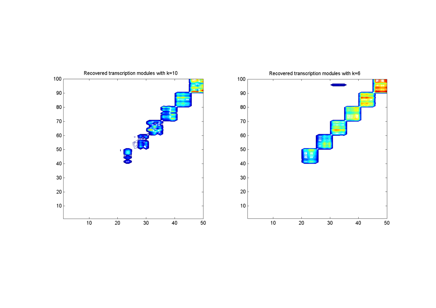
The iterated use of the LAROS algorithm of [6] to extract blocks one at a time, however, will not succeed in the case that there are two or more hidden blocks of roughly the same magnitude. In order to avoid this issue, we propose a new convex formulation that allows us to extract several (non-overlapping) features simultaneously. In Section 2, we study the proposed convex relaxation and the properties of its optimal solutions. In Section 3, we provide conditions to recover low-rank block structure of the block diagonal data matrix 𝑨A in the presence of random noise. Finally, we demonstrate our results with some numerical examples in Section 4, including a synthetic biclustering example and a synthetic gene expression example from the previous literature.

Notation. ⟨𝑨,𝑿⟩=trace​(𝑨T​𝑿)\langle\mbox{\boldmath$A$},{\boldsymbol{X}}\rangle=\mbox{trace}(\mbox{\boldmath$A$}^{T}{\boldsymbol{X}}) is used to denote the inner product of two matrices 𝑨A and 𝑿{\boldsymbol{X}} in ℝm×n\mathbb{R}^{m\times n}. ‖𝑿‖1\left\lVert{\boldsymbol{X}}\right\rVert_{1} means the sum of the absolute values of all entries of 𝑿{\boldsymbol{X}}, i.e., the ℓ1\ell_{1}-norm of vec​(𝑿)\mbox{vec}({\boldsymbol{X}}), the long vector constructed by the concatenation of all columns of 𝑿{\boldsymbol{X}}. Similarly, ‖𝑿‖∞\left\lVert{\boldsymbol{X}}\right\rVert_{\infty} is the maximum absolute value of entries of 𝑿{\boldsymbol{X}}, i.e, the ℓ∞\ell_{\infty}-norm of vec​(𝑿)\mbox{vec}({\boldsymbol{X}}).

2 Matrix norm minimization

We start with the following general norm minimization problem, which has been considered in [6].

min∥|𝑿|∥s.t.⟨𝑨,𝑿⟩≥1,\begin{array}[]{rl}\min&\lVert\mkern-2.0mu|{\boldsymbol{X}}|\mkern-2.0mu\rVert\\ \mathop{\rm s.t.}&\langle\mbox{\boldmath$A$},{\boldsymbol{X}}\rangle\geq 1,\end{array} (2.1)

where ∥|⋅|∥\lVert\mkern-2.0mu|\,\cdot\,|\mkern-2.0mu\rVert is an arbitrary norm function on ℝm×n\mathbb{R}^{m\times n}. The associated dual norm ∥|⋅|∥⋆\lVert\mkern-2.0mu|\,\cdot\,|\mkern-2.0mu\rVert^{\star} is defined as

∥|𝑨|∥⋆=max⟨𝑨,𝒀⟩s.t.∥|𝒀|∥≤1.\begin{array}[]{rl}\lVert\mkern-2.0mu|\mbox{\boldmath$A$}|\mkern-2.0mu\rVert^{\star}=\max&\langle\mbox{\boldmath$A$},{\boldsymbol{Y}}\rangle\\ \mathop{\rm s.t.}&\lVert\mkern-2.0mu|{\boldsymbol{Y}}|\mkern-2.0mu\rVert\leq 1.\end{array} (2.2)

These two optimization problems are closely related and their relationship is captured in the following lemmas and theorem discussed in Doan and Vavasis [6].

Lemma 1.

Matrix 𝐗∗{\boldsymbol{X}}^{*} is an optimal solution of Problem (2.1)(\ref{eq:gnorm}) if and only if 𝐘∗=(∥|𝐀|∥⋆)​𝐗∗{\boldsymbol{Y}}^{*}=\left(\lVert\mkern-2.0mu|\mbox{\boldmath$A$}|\mkern-2.0mu\rVert^{\star}\right){\boldsymbol{X}}^{*} is an optimal solution of Problem 2.2.

Lemma 2.

The set of all optimal solutions of Problem (2.2)(\ref{eq:dgnorm}) is the subdifferential of the dual norm function ∥|⋅|∥⋆\lVert\mkern-2.0mu|\,\cdot\,|\mkern-2.0mu\rVert^{\star} at 𝐀A, ∂∥|𝐀|∥⋆\partial\lVert\mkern-2.0mu|\mbox{\boldmath$A$}|\mkern-2.0mu\rVert^{\star}.

Theorem 1 (Doan and Vavasis [6]).

The following statements are true:

  1. (i)

    The set of optimal solutions of Problem (2.1)(\ref{eq:gnorm}) is (∥|𝑨|∥⋆)−1​∂∥|𝑨|∥⋆(\lVert\mkern-2.0mu|\mbox{\boldmath$A$}|\mkern-2.0mu\rVert^{\star})^{-1}\partial\lVert\mkern-2.0mu|\mbox{\boldmath$A$}|\mkern-2.0mu\rVert^{\star}, where ∂∥|⋅|∥⋆\partial\lVert\mkern-2.0mu|\,\cdot\,|\mkern-2.0mu\rVert^{\star} is the subdifferential of the dual norm function ∥|⋅|∥⋆\lVert\mkern-2.0mu|\,\cdot\,|\mkern-2.0mu\rVert^{\star}.

  2. (ii)

    Problem (2.1)(\ref{eq:gnorm}) has a unique optimal solution if and only if the dual norm function ∥|⋅|∥⋆\lVert\mkern-2.0mu|\,\cdot\,|\mkern-2.0mu\rVert^{\star} is differentiable at 𝐀A.

The LAROS problem in [6] belongs to a special class of (2.1)(\ref{eq:gnorm}) with parametric matrix norms of the form ∥|𝑿|∥θ=∥|𝑿|∥+θ​‖𝑿‖1\lVert\mkern-2.0mu|{\boldsymbol{X}}|\mkern-2.0mu\rVert_{\theta}=\lVert\mkern-2.0mu|\mbox{\boldmath$X$}|\mkern-2.0mu\rVert+\theta\|\mbox{\boldmath$X$}\|_{1} where ∥|⋅|∥\lVert\mkern-2.0mu|\,\cdot\,|\mkern-2.0mu\rVert is a unitarily invariant norm and θ\theta is a nonnegative parameter, θ≥0\theta\geq 0:

min∥|𝑿|∥+θ​‖𝑿‖1s.t.⟨𝑨,𝑿⟩≥1.\begin{array}[]{rl}\min&\lVert\mkern-2.0mu|\mbox{\boldmath$X$}|\mkern-2.0mu\rVert+\theta\|\mbox{\boldmath$X$}\|_{1}\\ \mathop{\rm s.t.}&\langle\mbox{\boldmath$A$},{\boldsymbol{X}}\rangle\geq 1.\end{array} (2.3)

A norm ∥|⋅|∥\lVert\mkern-2.0mu|\,\cdot\,|\mkern-2.0mu\rVert is unitarily invariant if ∥|𝑼​𝑿​𝑽|∥=∥|𝑿|∥\lVert\mkern-2.0mu|\mbox{\boldmath$U$}{\boldsymbol{X}}\mbox{\boldmath$V$}|\mkern-2.0mu\rVert=\lVert\mkern-2.0mu|{\boldsymbol{X}}|\mkern-2.0mu\rVert for all pairs of unitary matrices 𝑼U and 𝑽V (see, for example, Lewis [15] for more details). For the LAROS problem, ∥|𝑿|∥\lVert\mkern-2.0mu|{\boldsymbol{X}}|\mkern-2.0mu\rVert is the nuclear norm, ∥|𝑿|∥=‖𝑿‖∗\lVert\mkern-2.0mu|{\boldsymbol{X}}|\mkern-2.0mu\rVert=\left\lVert{\boldsymbol{X}}\right\rVert_{*}, which is the sum of singular values of 𝑿{\boldsymbol{X}}. In order to characterize the optimal solutions of (2.3)(\ref{eq:tnorm}), we need to compute the dual norm ∥|⋅|∥θ⋆\lVert\mkern-2.0mu|\,\cdot\,|\mkern-2.0mu\rVert_{\theta}^{\star}:

∥|𝑨|∥θ⋆=max⟨𝑨,𝒀⟩s.t.∥|𝒀|∥+θ​‖𝒀‖1≤1.\begin{array}[]{rl}\lVert\mkern-2.0mu|\mbox{\boldmath$A$}|\mkern-2.0mu\rVert_{\theta}^{\star}=\max&\langle\mbox{\boldmath$A$},{\boldsymbol{Y}}\rangle\\ \mathop{\rm s.t.}&\lVert\mkern-2.0mu|\mbox{\boldmath$Y$}|\mkern-2.0mu\rVert+\theta\|\mbox{\boldmath$Y$}\|_{1}\leq 1.\end{array} (2.4)

The following proposition, which is a straightforward generalization of Proposition 7 in [6], provides a dual formulation to compute ∥|⋅|∥θ⋆\lVert\mkern-2.0mu|\,\cdot\,|\mkern-2.0mu\rVert_{\theta}^{\star}.

Proposition 1.

The dual norm ∥|𝐀|∥θ⋆\lVert\mkern-2.0mu|\mbox{\boldmath$A$}|\mkern-2.0mu\rVert_{\theta}^{\star} with θ>0\theta>0 is the optimal value of the following optimization problem:

∥|𝑨|∥θ⋆=minmax⁡{∥|𝒀|∥⋆,θ−1​‖𝒁‖∞}s.t.𝒀+𝒁=𝑨.\begin{array}[]{rl}\lVert\mkern-2.0mu|\mbox{\boldmath$A$}|\mkern-2.0mu\rVert_{\theta}^{\star}=\min&\max\left\{\lVert\mkern-2.0mu|{\boldsymbol{Y}}|\mkern-2.0mu\rVert^{\star},\theta^{-1}\left\lVert\boldsymbol{Z}\right\rVert_{\infty}\right\}\\ \mathop{\rm s.t.}&{\boldsymbol{Y}}+\boldsymbol{Z}=\mbox{\boldmath$A$}.\end{array} (2.5)

The optimality conditions of (2.3)(\ref{eq:tnorm}) are described in the following proposition, which is again a generalization of Proposition 9 in [6].

Proposition 2.

Consider a feasible solution 𝐗{\boldsymbol{X}} of Problem (2.3)(\ref{eq:tnorm}). If there exists (𝐘,𝐙)({\boldsymbol{Y}},\boldsymbol{Z}) that satisfies the conditions below,

  1. (i)

    𝒀+𝒁=𝑨{\boldsymbol{Y}}+\boldsymbol{Z}=\mbox{\boldmath$A$} and ∥|𝒀|∥⋆=θ−1​‖𝒁‖∞\lVert\mkern-2.0mu|{\boldsymbol{Y}}|\mkern-2.0mu\rVert^{\star}=\theta^{-1}\left\lVert\boldsymbol{Z}\right\rVert_{\infty},

  2. (ii)

    𝑿∈α​∂∥|𝒀|∥⋆{\boldsymbol{X}}\in\alpha\partial\lVert\mkern-2.0mu|{\boldsymbol{Y}}|\mkern-2.0mu\rVert^{\star}, α≥0\alpha\geq 0,

  3. (iii)

    𝑿∈β​∂‖𝒁‖∞{\boldsymbol{X}}\in\beta\partial\left\lVert\boldsymbol{Z}\right\rVert_{\infty}, β≥0\beta\geq 0,

  4. (iv)

    α+θ​β=(‖𝑨‖θ∗)−1\alpha+\theta\beta=\left(\left\lVert\mbox{\boldmath$A$}\right\rVert^{*}_{\theta}\right)^{-1},

then 𝐗{\boldsymbol{X}} is an optimal solution of Problem (2.3)(\ref{eq:tnorm}). In addition, if

  1. (v)

    ∥|⋅|∥⋆\lVert\mkern-2.0mu|\,\cdot\,|\mkern-2.0mu\rVert^{\star} is differentiable at 𝒀{\boldsymbol{Y}} or ‖⋅‖∞\left\lVert\,\cdot\,\right\rVert_{\infty} is differentiable at 𝒁\boldsymbol{Z},

then 𝐗{\boldsymbol{X}} is the unique optimal solution.

The low-rank structure of solutions obtained from the LAROS problem comes from the fact that the dual norm of the nuclear norm is the spectral norm (or 22-norm), ‖𝑿‖=σ1​(𝑿)\left\lVert{\boldsymbol{X}}\right\rVert=\sigma_{1}({\boldsymbol{X}}), the largest singular value of 𝑿{\boldsymbol{X}}. More exactly, it is due to the structure of the subdifferential ∂‖⋅‖\partial\left\lVert\,\cdot\,\right\rVert. According to Ziȩtak [22], if 𝒀=𝑼𝚺𝑽T\mbox{\boldmath$Y$}=\mbox{\boldmath$U$}\mbox{\boldmath$\Sigma$}\mbox{\boldmath$V$}^{T} is a singular value decomposition of 𝒀Y and ss is the multiplicity of the largest singular value of 𝒀Y, the subdifferential ∂‖𝒀‖\partial\left\lVert\mbox{\boldmath$Y$}\right\rVert is written as follows:

∂‖𝒀‖={𝑼[𝑺𝟎𝟎𝟎]𝑽T:𝑺∈𝒮+s,‖𝑺‖∗=1},\partial\left\lVert\mbox{\boldmath$Y$}\right\rVert=\left\{\mbox{\boldmath$U$}\begin{bmatrix}\mbox{\boldmath$S$}&\mbox{\boldmath$0$}\cr\mbox{\boldmath$0$}&\mbox{\boldmath$0$}\end{bmatrix}\mbox{\boldmath$V$}^{T}:\mbox{\boldmath$S$}\in{\cal S}^{s}_{+},\left\lVert\mbox{\boldmath$S$}\right\rVert_{*}=1\right\},

where 𝒮+s{\cal S}^{s}_{+} is the set of positive semidefinite matrices of size ss. The description of the subdifferential shows that the maximum possible rank of 𝑿∈α​∂‖𝒀‖{\boldsymbol{X}}\in\alpha\partial\left\lVert{\boldsymbol{Y}}\right\rVert is the multiplicity of the largest singular value of 𝒀Y and if s=1s=1, we achieve rank-one solutions. This structural property of the subdifferential ∂‖⋅‖\partial\left\lVert\,\cdot\,\right\rVert motivates the norm optimization formulation for the LAROS problem, which aims to find a single approximately rank-one submatrix of the data matrix 𝑨A. We now propose a new pair of norms that would allow us to handle several approximately rank-one submatrices simultaneously instead of individual ones. Let consider the following norm, which we call Ky Fan 22-kk-norm given its similar formulation to that of the classical Ky Fan kk-norm:

∥|𝑨|∥k,2=(∑i=1kσi2​(𝑨))12,\lVert\mkern-2.0mu|\mbox{\boldmath$A$}|\mkern-2.0mu\rVert_{k,2}=\left(\sum_{i=1}^{k}\sigma_{i}^{2}(\mbox{\boldmath$A$})\right)^{\frac{1}{2}}, (2.6)

where σ1≥…​σk≥0\sigma_{1}\geq\ldots\sigma_{k}\geq 0 are the first kk largest singular values of 𝑨A, k≤k0=rank​(𝑨)k\leq k_{0}=\mbox{rank}(\mbox{\boldmath$A$}). The dual norm of the Ky Fan 22-kk-norm is denoted by ∥|⋅|∥k,2⋆\lVert\mkern-2.0mu|\,\cdot\,|\mkern-2.0mu\rVert_{k,2}^{\star}. According to Bhatia [3], Ky Fan 22-kk-norm is a Q-norm, which is unitarily invariant (Definition IV.2.9 [3]). Since Ky Fan 22-kk-norm is unitarily invariant, we can define its corresponding symmetric gauge function, ‖⋅‖k,2:ℝn→ℝ\left\lVert\,\cdot\,\right\rVert_{k,2}:\mathbb{R}^{n}\rightarrow\mathbb{R}, as follows:

‖𝒙‖k,2=(∑i=1k|x|(i)2)12,\left\lVert{\boldsymbol{x}}\right\rVert_{k,2}=\left(\sum_{i=1}^{k}\left\lvert x\right\rvert_{(i)}^{2}\right)^{\frac{1}{2}}, (2.7)

where |x|(i)\left\lvert x\right\rvert_{(i)} is the (n−i+1)(n-i+1)-st order statistic of |𝒙|\left\lvert{\boldsymbol{x}}\right\rvert. The dual norm of this gauge function (or more exactly, its square), has been used in Argyriou et al. [2] as a regularizer in sparse prediction problems. More recently, its matrix counterpart is considered in McDonald et al. [17] as a special case of the matrix cluster norm defined in [13], whose square is used for multi-task learning regularization. On the other hand, the square Ky Fan 22-kk-norm is considered as a penalty in low-rank regression analysis in Giraud [8]. In this paper, we are going to use dual Ky Fan 22-kk-norm, not its square, in our formulation given its structural properties, which will be explained later.

When k=1k=1, the Ky Fan 22-kk-norm becomes the spectral norm, whose subdifferential has been used to characterize the low-rank structure of the optimal solutions of the LAROS problem. We now propose the following optimization problem, of which the LAROS problem is a special instance with k=1k=1:

min∥|𝑿|∥k,2⋆+θ​‖𝑿‖1s.t.⟨𝑨,𝑿⟩≥1,\begin{array}[]{rl}\min&\lVert\mkern-2.0mu|{\boldsymbol{X}}|\mkern-2.0mu\rVert_{k,2}^{\star}+\theta\left\lVert{\boldsymbol{X}}\right\rVert_{1}\\ \mathop{\rm s.t.}&\langle\mbox{\boldmath$A$},{\boldsymbol{X}}\rangle\geq 1,\end{array} (2.8)

where θ\theta is a nonnegative parameter, θ≥0\theta\geq 0. The proposed formulation is an instance of the parametric problem (2.3)(\ref{eq:tnorm}) and we can use results obtained in Proposition 1 and 2 to characterize its optimal solutions. Before doing so, we first provide an equivalent semidefinite optimization formulation for (2.8)(\ref{eq:nprob}) in the following proposition.

Proposition 3.

Assuming m≥nm\geq n, the optimization problem (2.8)(\ref{eq:nprob}) is then equivalent to the following semidefinite optimization problem:

minp,𝑷,𝑸,𝑹,𝑿p+trace​(𝑹)+θ​⟨𝑬,𝑸⟩s.t.k​p−trace​(𝑷)=0,p​𝑰−𝑷⪰0,(𝑷−12​𝑿T−12​𝑿𝑹)⪰0,𝑸≥𝑿,𝑸≥−𝑿,⟨𝑨,𝑿⟩≥1,\begin{array}[]{rl}\displaystyle\min_{p,{\boldsymbol{P}},{\boldsymbol{Q}},{\boldsymbol{R}},{\boldsymbol{X}}}&p+\mbox{trace}(\mbox{\boldmath$R$})+\theta\langle\mbox{\boldmath$E$},\mbox{\boldmath$Q$}\rangle\\ \mathop{\rm s.t.}&kp-\mbox{trace}(\mbox{\boldmath$P$})=0,\\ &p\mbox{\boldmath$I$}-\mbox{\boldmath$P$}\succeq 0,\\ &\begin{pmatrix}\mbox{\boldmath$P$}&-\frac{1}{2}\mbox{\boldmath$X$}^{T}\\ -\frac{1}{2}\mbox{\boldmath$X$}&\mbox{\boldmath$R$}\end{pmatrix}\succeq 0,\\ &\mbox{\boldmath$Q$}\geq{\boldsymbol{X}},\,\mbox{\boldmath$Q$}\geq-{\boldsymbol{X}},\\ &\langle\mbox{\boldmath$A$},{\boldsymbol{X}}\rangle\geq 1,\end{array} (2.9)

where 𝐄E is the matrix of all ones.

Proof. We first consider the dual norm ∥|𝑿|∥k,2⋆\lVert\mkern-2.0mu|{\boldsymbol{X}}|\mkern-2.0mu\rVert_{k,2}^{\star}. We have:

∥|𝑿|∥k,2⋆=max⟨𝑿,𝒀⟩s.t.∥|𝒀|∥k,2≤1.\begin{array}[]{rl}\lVert\mkern-2.0mu|\mbox{\boldmath$X$}|\mkern-2.0mu\rVert^{\star}_{k,2}=\displaystyle\max&\langle\mbox{\boldmath$X$},{\boldsymbol{Y}}\rangle\\ \mathop{\rm s.t.}&\lVert\mkern-2.0mu|{\boldsymbol{Y}}|\mkern-2.0mu\rVert_{k,2}\leq 1.\end{array} (2.10)

Since m≥nm\geq n, we have: (∥|𝒀|∥k,2)2=∥|𝒀T​𝒀|∥k\left(\lVert\mkern-2.0mu|{\boldsymbol{Y}}|\mkern-2.0mu\rVert_{k,2}\right)^{2}=\lVert\mkern-2.0mu|{\boldsymbol{Y}}^{T}{\boldsymbol{Y}}|\mkern-2.0mu\rVert_{k}, where ∥|⋅|∥k\lVert\mkern-2.0mu|\,\cdot\mathcal{|}\mkern-2.0mu\rVert_{k} is the Ky Fan kk-norm, i.e., the sum of kk largest singular values. Since 𝒀T​𝒀{\boldsymbol{Y}}^{T}{\boldsymbol{Y}} is symmetric, ∥|𝒀T​𝒀|∥k\lVert\mkern-2.0mu|{\boldsymbol{Y}}^{T}{\boldsymbol{Y}}|\mkern-2.0mu\rVert_{k} is actually the sum of kk largest eigenvalues of 𝒀T​𝒀{\boldsymbol{Y}}^{T}{\boldsymbol{Y}}. Similar to ‖𝒙‖k\left\lVert{\boldsymbol{x}}\right\rVert_{k}, which is the sum of kk largest elements of 𝒙{\boldsymbol{x}}, we obtain the following (dual) optimization formulation for ∥|𝒀T​𝒀|∥k\lVert\mkern-2.0mu|{\boldsymbol{Y}}^{T}{\boldsymbol{Y}}|\mkern-2.0mu\rVert_{k} (for example, see Laurent and Rendl [14]):

∥|𝒀T​𝒀|∥k=mink​z+trace​(𝑼)s.t.z​𝑰+𝑼⪰𝒀T​𝒀,𝑼⪰0.\begin{array}[]{rl}\lVert\mkern-2.0mu|{\boldsymbol{Y}}^{T}{\boldsymbol{Y}}|\mkern-2.0mu\rVert_{k}=\min&kz+\mbox{trace}(\mbox{\boldmath$U$})\\ \mathop{\rm s.t.}&z\mbox{\boldmath$I$}+\mbox{\boldmath$U$}\succeq{\boldsymbol{Y}}^{T}{\boldsymbol{Y}},\\ &\mbox{\boldmath$U$}\succeq 0.\end{array}

Applying the Schur complement, we have:

∥|𝒀T​𝒀|∥k=mink​z+trace​(𝑼)s.t.(z​𝑰+𝑼𝒀T𝒀𝑰)⪰0,𝑼⪰0.\begin{array}[]{rl}\lVert\mkern-2.0mu|{\boldsymbol{Y}}^{T}{\boldsymbol{Y}}|\mkern-2.0mu\rVert_{k}=\min&kz+\mbox{trace}(\mbox{\boldmath$U$})\\ \mathop{\rm s.t.}&\begin{pmatrix}z\mbox{\boldmath$I$}+\mbox{\boldmath$U$}&{\boldsymbol{Y}}^{T}\\ {\boldsymbol{Y}}&\mbox{\boldmath$I$}\end{pmatrix}\succeq 0,\\ &\mbox{\boldmath$U$}\succeq 0.\end{array}

Thus, the dual norm ∥|⋅|∥k,2⋆\lVert\mkern-2.0mu|\,\cdot\,|\mkern-2.0mu\rVert_{k,2}^{\star} can be computed as follows:

∥|𝑿|∥k,2⋆=max⟨𝑿,𝒀⟩s.t.k​z+trace​(𝑼)≤1,(z​𝑰+𝑼𝒀T𝒀𝑰)⪰0,𝑼⪰0.\begin{array}[]{rl}\lVert\mkern-2.0mu|\mbox{\boldmath$X$}|\mkern-2.0mu\rVert_{k,2}^{\star}=\max&\langle\mbox{\boldmath$X$},{\boldsymbol{Y}}\rangle\\ \mathop{\rm s.t.}&kz+\mbox{trace}(\mbox{\boldmath$U$})\leq 1,\\ &\begin{pmatrix}z\mbox{\boldmath$I$}+\mbox{\boldmath$U$}&{\boldsymbol{Y}}^{T}\\ {\boldsymbol{Y}}&\mbox{\boldmath$I$}\end{pmatrix}\succeq 0,\\ &\mbox{\boldmath$U$}\succeq 0.\end{array}

Applying strong duality theory under Slater’s condition, we have:

∥|𝑿|∥k,2⋆=minp+trace​(𝑹)s.t.k​p−trace​(𝑷)=0,p​𝑰−𝑷⪰0,(𝑷−12​𝑿T−12​𝑿𝑹)⪰0.\begin{array}[]{rl}\lVert\mkern-2.0mu|\mbox{\boldmath$X$}|\mkern-2.0mu\rVert_{k,2}^{\star}=\min&p+\mbox{trace}(\mbox{\boldmath$R$})\\ \mathop{\rm s.t.}&kp-\mbox{trace}(\mbox{\boldmath$P$})=0,\\ &p\mbox{\boldmath$I$}-\mbox{\boldmath$P$}\succeq 0,\\ &\begin{pmatrix}\mbox{\boldmath$P$}&-\frac{1}{2}\mbox{\boldmath$X$}^{T}\\ -\frac{1}{2}\mbox{\boldmath$X$}&\mbox{\boldmath$R$}\end{pmatrix}\succeq 0.\end{array} (2.11)

The reformulation of ‖𝑿‖1\left\lVert{\boldsymbol{X}}\right\rVert_{1} is straightforward with the new decision variable 𝑸Q and additional constraints 𝑸≥𝑿\mbox{\boldmath$Q$}\geq{\boldsymbol{X}} and 𝑸≥−𝑿\mbox{\boldmath$Q$}\geq-{\boldsymbol{X}}, given the fact that the main problem is a minimization problem. □\square

Proposition 3 indicates that in general, we can solve (2.8)(\ref{eq:nprob}) by solving its equivalent semidefinite optimization formulation (2.9)(\ref{eq:sdpprob}) with any SDP solver. We are now ready to study some properties of optimal solutions of (2.8)(\ref{eq:nprob}). We have: ∥|𝑿|∥k,2⋆+θ​‖𝑿‖1\lVert\mkern-2.0mu|{\boldsymbol{X}}|\mkern-2.0mu\rVert_{k,2}^{\star}+\theta\left\lVert{\boldsymbol{X}}\right\rVert_{1} is a norm for θ≥0\theta\geq 0 and we denote it by ∥|𝑿|∥k,2,θ\lVert\mkern-2.0mu|{\boldsymbol{X}}|\mkern-2.0mu\rVert_{k,2,\theta}. According to Proposition 1, the dual norm ∥|𝑿|∥k,2,θ⋆\lVert\mkern-2.0mu|{\boldsymbol{X}}|\mkern-2.0mu\rVert_{k,2,\theta}^{\star},

∥|𝑨|∥k,2,θ⋆=max⟨𝑨,𝑿⟩s.t.‖𝑿‖k,2,θ≤1,\begin{array}[]{rl}\lVert\mkern-2.0mu|\mbox{\boldmath$A$}|\mkern-2.0mu\rVert^{\star}_{k,2,\theta}=\displaystyle\max&\langle\mbox{\boldmath$A$},{\boldsymbol{X}}\rangle\\ \mathop{\rm s.t.}&\left\lVert{\boldsymbol{X}}\right\rVert_{k,2,\theta}\leq 1,\end{array} (2.12)

can be calculated by solving the following optimization problem given θ>0\theta>0:

∥|𝑨|∥k,2,θ⋆=minmax⁡{∥|𝒀|∥k,2,θ−1​‖𝒁‖∞}s.t.𝒀+𝒁=𝑨.\begin{array}[]{rl}\lVert\mkern-2.0mu|\mbox{\boldmath$A$}|\mkern-2.0mu\rVert_{k,2,\theta}^{\star}=\min&\max\left\{\lVert\mkern-2.0mu|{\boldsymbol{Y}}|\mkern-2.0mu\rVert_{k,2},\theta^{-1}\left\lVert\boldsymbol{Z}\right\rVert_{\infty}\right\}\\ \mathop{\rm s.t.}&{\boldsymbol{Y}}+\boldsymbol{Z}=\mbox{\boldmath$A$}.\end{array} (2.13)

Similar to Proposition 2, we can provide the optimality conditions for (2.8)(\ref{eq:nprob}) in the following proposition.

Proposition 4.

Consider a feasible solution 𝐗{\boldsymbol{X}} of Problem (2.8)(\ref{eq:nprob}). If there exists (𝐘,𝐙)({\boldsymbol{Y}},\boldsymbol{Z}) that satisfies the conditions below,

  1. (i)

    𝒀+𝒁=𝑨{\boldsymbol{Y}}+\boldsymbol{Z}=\mbox{\boldmath$A$} and ∥|𝒀|∥k,2=θ−1​‖𝒁‖∞\lVert\mkern-2.0mu|{\boldsymbol{Y}}|\mkern-2.0mu\rVert_{k,2}=\theta^{-1}\left\lVert\boldsymbol{Z}\right\rVert_{\infty},

  2. (ii)

    𝑿∈α​∂∥|𝒀|∥k,2{\boldsymbol{X}}\in\alpha\partial\lVert\mkern-2.0mu|{\boldsymbol{Y}}|\mkern-2.0mu\rVert_{k,2}, α≥0\alpha\geq 0,

  3. (iii)

    𝑿∈β​∂‖𝒁‖∞{\boldsymbol{X}}\in\beta\partial\left\lVert\boldsymbol{Z}\right\rVert_{\infty}, β≥0\beta\geq 0,

  4. (iv)

    α+θ​β=(‖𝑨‖k,2,θ∗)−1\alpha+\theta\beta=\left(\left\lVert\mbox{\boldmath$A$}\right\rVert^{*}_{k,2,\theta}\right)^{-1},

then 𝐗{\boldsymbol{X}} is an optimal solution of Problem (2.3)(\ref{eq:tnorm}). In addition, if

  1. (v)

    ∥|⋅|∥k,2\lVert\mkern-2.0mu|\,\cdot\,|\mkern-2.0mu\rVert_{k,2} is differentiable at 𝒀{\boldsymbol{Y}} or ‖⋅‖∞\left\lVert\,\cdot\,\right\rVert_{\infty} is differentiable at 𝒁\boldsymbol{Z},

then 𝐗{\boldsymbol{X}} is the unique optimal solution.

The optimality conditions presented in Proposition 4 indicate that some properties of optimal solutions of (2.8)(\ref{eq:nprob}) can be derived from the structure of ∂∥|⋅|∥k,2\partial\lVert\mkern-2.0mu|\,\cdot\,|\mkern-2.0mu\rVert_{k,2}. We shall characterize the subdifferential ∂∥|⋅|∥k,2\partial\lVert\mkern-2.0mu|\,\cdot\,|\mkern-2.0mu\rVert_{k,2} next. According to Watson [21], since ∥|⋅|∥k,2\lVert\mkern-2.0mu|\,\cdot\,|\mkern-2.0mu\rVert_{k,2} is a unitarily invariant norm, ∂∥|𝑨|∥k,2\partial\lVert\mkern-2.0mu|\mbox{\boldmath$A$}|\mkern-2.0mu\rVert_{k,2} is related to ∂‖σ⁡(𝑨)‖k,2\partial\left\lVert\sigma(\mbox{\boldmath$A$})\right\rVert_{k,2}, where σ⁡(𝑨)\sigma(\mbox{\boldmath$A$}) is the vector of singular values of 𝑨A. Let 𝑨≠𝟎\mbox{\boldmath$A$}\neq\mbox{\boldmath$0$} be a matrix with singular values that satisfy

σ1≥…>σk−t+1=…=σk=…=σk+s>…≥σp,\sigma_{1}\geq\ldots>\sigma_{k-t+1}=\ldots=\sigma_{k}=\ldots=\sigma_{k+s}>\ldots\geq\sigma_{p},

where p=min⁡{m,n}p=\min\{m,n\}, so that the multiplicity of σk\sigma_{k} is s+ts+t. The subdifferential ∂‖𝝈‖k,2\partial\left\lVert\mbox{\boldmath$\sigma$}\right\rVert_{k,2} is characterized in the following lemma.

Lemma 3.

𝒗∈∂‖𝝈‖k,2\mbox{\boldmath$v$}\in\partial\left\lVert\mbox{\boldmath$\sigma$}\right\rVert_{k,2} if and only 𝐯v satisfies the following conditions:

  1. (i)

    vi=σi‖𝝈‖k,2\displaystyle v_{i}=\frac{\sigma_{i}}{\left\lVert\mbox{\boldmath$\sigma$}\right\rVert_{k,2}} for all i=1,…,k−ti=1,\ldots,k-t.

  2. (ii)

    vi=τi​σk‖𝝈‖k,2\displaystyle v_{i}=\tau_{i}\frac{\sigma_{k}}{\left\lVert\mbox{\boldmath$\sigma$}\right\rVert_{k,2}}, 0≤τi≤10\leq\tau_{i}\leq 1 for all i=k−t+1,…,k+si=k-t+1,\ldots,k+s, and ∑i=k−t+1k+sτi=t\displaystyle\sum_{i=k-t+1}^{k+s}\tau_{i}=t.

  3. (iii)

    vi=0v_{i}=0 for all i=k+s+1,…,pi=k+s+1,\ldots,p.

Proof. Let 𝒩k{\cal N}_{k} be the collection of all subsets with kk elements of {1,…,p}\{1,\ldots,p\}, we have:

‖𝝈‖k,2=maxN∈𝒩k⁡fN​(𝝈),\left\lVert\mbox{\boldmath$\sigma$}\right\rVert_{k,2}=\max_{N\in{\cal N}_{k}}f_{N}(\mbox{\boldmath$\sigma$}),

where fN​(𝝈)=(∑i∈Nσi2)12\displaystyle f_{N}(\mbox{\boldmath$\sigma$})=\left(\sum_{i\in N}\sigma_{i}^{2}\right)^{\frac{1}{2}} for all N∈𝒩kN\in{\cal N}_{k}. According to Dubovitski-Milyutin’s theorem (see, for example, Tikhomirov [20]), the subdifferential of ‖⋅‖k,2\left\lVert\,\cdot\,\right\rVert_{k,2} is computed as follows:

∂‖𝝈‖k,2=conv{∂fN(𝝈):N∈𝒩k,fN(𝝈)=‖𝝈‖k,2}.\partial\left\lVert\mbox{\boldmath$\sigma$}\right\rVert_{k,2}=\mbox{conv}\left\{\partial f_{N}(\mbox{\boldmath$\sigma$})\,:\,N\in{\cal N}_{k},\,f_{N}(\mbox{\boldmath$\sigma$})=\left\lVert\mbox{\boldmath$\sigma$}\right\rVert_{k,2}\right\}.

With the structure of 𝝈\sigma, clearly {1,…,k−t}∈N\{1,\ldots,k-t\}\in N for all N∈𝒩kN\in{\cal N}_{k} such that fN​(𝝈)=‖𝝈‖k,2f_{N}(\mbox{\boldmath$\sigma$})=\left\lVert\mbox{\boldmath$\sigma$}\right\rVert_{k,2}. The remaining tt elements of NN are chosen from s+ts+t values from {k−t+1,…,k+s}\{k-t+1,\ldots,k+s\}. Since 𝝈≠𝟎\mbox{\boldmath$\sigma$}\neq\mbox{\boldmath$0$}, all fNf_{N} that satisfy fN​(𝝈)=‖𝝈‖k,2f_{N}(\mbox{\boldmath$\sigma$})=\left\lVert\mbox{\boldmath$\sigma$}\right\rVert_{k,2} is differentiable at 𝝈\sigma (even in the case σk=0\sigma_{k}=0) and

∂fN​(𝝈)∂σi=σi‖𝝈‖k,2,∀i∈N,∂fN​(𝝈)∂σi=0,i∉N.\frac{\partial f_{N}(\mbox{\boldmath$\sigma$})}{\partial\sigma_{i}}=\frac{\sigma_{i}}{\left\lVert\mbox{\boldmath$\sigma$}\right\rVert_{k,2}},\,\forall\,i\in N,\hskip 10.00002pt\frac{\partial f_{N}(\mbox{\boldmath$\sigma$})}{\partial\sigma_{i}}=0,\,\hskip 10.00002pt\,i\not\in N.

Thus if 𝒗∈∂‖𝝈‖k,2\mbox{\boldmath$v$}\in\partial\left\lVert\mbox{\boldmath$\sigma$}\right\rVert_{k,2}, for all i=1,…,k−ti=1,\ldots,k-t, we have: vi=σi‖𝝈‖k,2\displaystyle v_{i}=\frac{\sigma_{i}}{\left\lVert\mbox{\boldmath$\sigma$}\right\rVert_{k,2}} and vi=0v_{i}=0 for all i=k+s+1,…,pi=k+s+1,\ldots,p.

We now have: counting arguments for the appearance of each index in {k−t+1,…,k+s}\{k-t+1,\ldots,k+s\} with respect to all subsets N∈𝒩kN\in{\cal N}_{k} that satisfy fN​(𝝈)=‖𝝈‖k,2f_{N}(\mbox{\boldmath$\sigma$})=\left\lVert\mbox{\boldmath$\sigma$}\right\rVert_{k,2} allow us to characterize viv_{i} for i=k−t+1,…,k+si=k-t+1,\ldots,k+s as vi=τi​σk‖𝝈‖k,2\displaystyle v_{i}=\tau_{i}\frac{\sigma_{k}}{\left\lVert\mbox{\boldmath$\sigma$}\right\rVert_{k,2}}, 0≤τi≤10\leq\tau_{i}\leq 1 and ∑i=k−t+1k+sτi=t\displaystyle\sum_{i=k-t+1}^{k+s}\tau_{i}=t. □\square

We are ready to characterize the subdifferential of ∥|⋅|∥k,2\lVert\mkern-2.0mu|\,\cdot\,|\mkern-2.0mu\rVert_{k,2} with the following proposition.

Proposition 5.

Consider 𝐀≠𝟎\mbox{\boldmath$A$}\neq\mbox{\boldmath$0$}. Let 𝐀=𝐔𝚺𝐕T\mbox{\boldmath$A$}=\mbox{\boldmath$U$}\mbox{\boldmath$\Sigma$}\mbox{\boldmath$V$}^{T} be a particular singular value decomposition of 𝐀A and assume that σ⁡(𝐀)\sigma(\mbox{\boldmath$A$}) satisfies σ1≥…>σk−t+1=…=σk=…=σk+s>…≥σp\sigma_{1}\geq\ldots>\sigma_{k-t+1}=\ldots=\sigma_{k}=\ldots=\sigma_{k+s}>\ldots\geq\sigma_{p}. Then, 𝐆∈∂∥|𝐀|∥k,2\mbox{\boldmath$G$}\in\partial\lVert\mkern-2.0mu|\mbox{\boldmath$A$}|\mkern-2.0mu\rVert_{k,2} if and only if there exists 𝐓∈ℝ(s+t)×(s+t)\mbox{\boldmath$T$}\in\mathbb{R}^{(s+t)\times(s+t)} such that

𝑮=1∥|𝑨|∥k,2(𝑼[:,1:k−t]𝚺[1:k−t,1:k−t]𝑽[:,1:k−t]T+σk𝑼[:,k−t+1:k+s]𝐓𝐕[:,k−t+1:k+s]T),\mbox{\boldmath$G$}=\frac{1}{\lVert\mkern-2.0mu|\mbox{\boldmath$A$}|\mkern-2.0mu\rVert_{k,2}}\left(\mbox{\boldmath$U$}_{[:,1:k-t]}\mbox{\boldmath$\Sigma$}_{[1:k-t,1:k-t]}\mbox{\boldmath$V$}_{[:,1:k-t]}^{T}+\sigma_{k}\mbox{\boldmath$U$}_{[:,k-t+1:k+s]}\mbox{\boldmath$T$}\mbox{\boldmath$V$}_{[:,k-t+1:k+s]}^{T}\right),

where 𝐓T is symmetric positive semidefinite, ‖𝐓‖≤1\left\lVert\mbox{\boldmath$T$}\right\rVert\leq 1 and ‖𝐓‖∗=t\left\lVert\mbox{\boldmath$T$}\right\rVert_{*}=t.

Proof. According to Watson [21], we have:

∂∥|𝑨|∥k,2={𝑼Diag(𝒈)𝑽T:𝑨=𝑼𝚺𝑽Tis any SVD of𝑨,𝒈∈∂‖σ(𝑨)‖k,2}.\partial\lVert\mkern-2.0mu|\mbox{\boldmath$A$}|\mkern-2.0mu\rVert_{k,2}=\left\{\mbox{\boldmath$U$}\mbox{Diag}(\mbox{\boldmath$g$})\mbox{\boldmath$V$}^{T}:\,\mbox{\boldmath$A$}=\mbox{\boldmath$U$}\mbox{\boldmath$\Sigma$}\mbox{\boldmath$V$}^{T}\,\mbox{is any SVD of}\,\mbox{\boldmath$A$},\,\mbox{\boldmath$g$}\in\partial\left\lVert\sigma(\mbox{\boldmath$A$})\right\rVert_{k,2}\right\}.

Let 𝑨=𝑼𝚺𝑽T\mbox{\boldmath$A$}=\mbox{\boldmath$U$}\mbox{\boldmath$\Sigma$}\mbox{\boldmath$V$}^{T} be a particular singular value decomposition of 𝑨A and assume that a singular value σi>0\sigma_{i}>0 has the multiplicity of rr with corresponding singular vectors 𝑼i∈ℝm×r\mbox{\boldmath$U$}_{i}\in\mathbb{R}^{m\times r} and 𝑽i∈ℝn×r\mbox{\boldmath$V$}_{i}\in\mathbb{R}^{n\times r}. Then for any singular value decomposition of 𝑨A, 𝑨=𝑼¯​𝚺​𝑽¯T\mbox{\boldmath$A$}=\bar{\mbox{\boldmath$U$}}\mbox{\boldmath$\Sigma$}\bar{\mbox{\boldmath$V$}}^{T}, there exists an orthonormal matrix 𝑾∈ℝr×r\mbox{\boldmath$W$}\in\mathbb{R}^{r\times r}, 𝑾𝑾T=𝑰\mbox{\boldmath$W$}\mbox{\boldmath$W$}^{T}=\mbox{\boldmath$I$}, such that 𝑼¯i=𝑼i​𝑾\bar{\mbox{\boldmath$U$}}_{i}=\mbox{\boldmath$U$}_{i}\mbox{\boldmath$W$} and 𝑽¯i=𝑽i​𝑾\bar{\mbox{\boldmath$V$}}_{i}=\mbox{\boldmath$V$}_{i}\mbox{\boldmath$W$} (for example, see Ziȩtak [22]).

Combining these results with Lemma 3, the proof is straightforward with a singular value (or eigenvalue) decomposition of matrix 𝑻T. □\square

Corollary 1.

∥|⋅|∥k,2\lVert\mkern-2.0mu|\,\cdot\,|\mkern-2.0mu\rVert_{k,2} is differentiable at any 𝐀≠𝟎\mbox{\boldmath$A$}\neq\mbox{\boldmath$0$} such that σk>σk+1\sigma_{k}>\sigma_{k+1} (σp+1=0\sigma_{p+1}=0) or σk=0\sigma_{k}=0.

Proof. If σk=0\sigma_{k}=0, then, according to Proposition 5,

𝑮∈∂∥|𝑨|∥k,2⇔𝑮=1∥|𝑨|∥k,2𝑼[:,1:k−t]𝚺[1:k−t,1:k−t]𝑽[:,1:k−t]T.\mbox{\boldmath$G$}\in\partial\lVert\mkern-2.0mu|\mbox{\boldmath$A$}|\mkern-2.0mu\rVert_{k,2}\,\Leftrightarrow\,\mbox{\boldmath$G$}=\frac{1}{\lVert\mkern-2.0mu|\mbox{\boldmath$A$}|\mkern-2.0mu\rVert_{k,2}}\mbox{\boldmath$U$}_{[:,1:k-t]}\mbox{\boldmath$\Sigma$}_{[1:k-t,1:k-t]}\mbox{\boldmath$V$}_{[:,1:k-t]}^{T}.

Now, if σk>σk+1\sigma_{k}>\sigma_{k+1}, we have: s=0s=0, thus 𝑻=𝑰\mbox{\boldmath$T$}=\mbox{\boldmath$I$} is unique since 𝑻∈𝒮t\mbox{\boldmath$T$}\in{\cal S}^{t}, ‖𝑻‖∗=t\left\lVert\mbox{\boldmath$T$}\right\rVert_{*}=t, and ‖𝑻‖≤1\left\lVert\mbox{\boldmath$T$}\right\rVert\leq 1. Thus ∂∥|𝑨|∥k,2\partial\lVert\mkern-2.0mu|\mbox{\boldmath$A$}|\mkern-2.0mu\rVert_{k,2} is a singleton, which implies ∥|⋅|∥k,2\lVert\mkern-2.0mu|\,\cdot\,|\mkern-2.0mu\rVert_{k,2} is differentiable at 𝑨A. □\square

Proposition 5 shows that the problem (2.8)(\ref{eq:nprob}) with θ=0\theta=0 is a convex optimization problem that finds kk-approximation of a matrix 𝑨A. It also shows that intuitively, the problem (2.8)(\ref{eq:nprob}) can be used to recover kk largest approximately rank-one submatrices with θ>0\theta>0. Note that for Ky Fan kk-norm, if σk​(𝑨)>σk+1​(𝑨)\sigma_{k}(\mbox{\boldmath$A$})>\sigma_{k+1}(\mbox{\boldmath$A$}), its subdifferential at 𝑨A is a singleton with a unique subgradient:

∂∥|𝑨|∥k={𝑼​[𝑰k𝟎𝟎𝟎]​𝑽T},\partial\lVert\mkern-2.0mu|\mbox{\boldmath$A$}|\mkern-2.0mu\rVert_{k}=\left\{\mbox{\boldmath$U$}\begin{bmatrix}\mbox{\boldmath$I$}_{k}&\mbox{\boldmath$0$}\cr\mbox{\boldmath$0$}&\mbox{\boldmath$0$}\end{bmatrix}\mbox{\boldmath$V$}^{T}\right\},

where 𝑨=𝑼​Σ​𝑽T\mbox{\boldmath$A$}=\mbox{\boldmath$U$}\Sigma\mbox{\boldmath$V$}^{T} is a singular value decomposition of 𝑨A and 𝑰k\mbox{\boldmath$I$}_{k} is the identity matrix in ℝk×k\mathbb{R}^{k\times k} (see for example, Watson [21]). In this particular case, the unique subgradient of the Ky Fan kk-norm provides the information of singular vectors corresponding to the kk largest singular values. Having said that, it does not preserve the information of singular values. When θ=0\theta=0, the proposed formulation with the Ky Fan kk-norm will not return the rank-kk approximation of the matrix 𝑨A as the Ky Fan 22-kk-norm does. In the next section, we shall study the recovery of these submatrices under the presence of random noise.

3 Recovery with Block Diagonal Matrices and Random Noise

We consider 𝑨=𝑩+𝑹\mbox{\boldmath$A$}=\mbox{\boldmath$B$}+\mbox{\boldmath$R$}, where 𝑩B is a block diagonal matrix, each block having rank one, while 𝑹R is a noise matrix. The main theorem shows that under certain assumptions concerning the noise, the positions of the blocks can be recovered from the solution of (2.8)(\ref{eq:nprob}). As mentioned in the introduction, this corresponds to solving a special case of the approximate NMF problem, that is, a factorization 𝑨≈𝑾𝑯T\mbox{\boldmath$A$}\approx\mbox{\boldmath$W$}\mbox{\boldmath$H$}^{T}, where 𝑾W and 𝑯H are nonnegative matrices. The special case solved is that 𝑾W and 𝑯H each consist of nonnegative columns with nonzeros in disjoint positions (so that 𝑨A is approximately a matrix with disjoint blocks each of rank one). Even this special case of NMF is NP-hard unless further restrictions are placed on the data model given the fact that the (exact) LAROS problem is NP-hard (see [6] for details).

Before starting the proof of the theorem, we need to consider some properties of subgaussian random variables. A random variable xx is bb-subgaussian if 𝔼⁡[x]=0\mathbb{E}[x]=0 and there exists a b>0b>0 such that for all t∈ℝt\in\mathbb{R},

𝔼⁡[et​x]≤eb2​t22.\mathbb{E}\left[e^{tx}\right]\leq e^{\frac{b^{2}t^{2}}{2}}. (3.1)

We can apply the Markov inequality for the bb-subgaussian random variable xx and obtain the following inequalities:

ℙ(x≥t)≤exp(−t2/(2b2)) and ℙ(x≤−t)≤exp(−t2/(2b2)),∀t>0.\mathbb{P}(x\geq t)\leq\exp(-t^{2}/(2b^{2}))\mbox{ and }\mathbb{P}(x\leq-t)\leq\exp(-t^{2}/(2b^{2})),\hskip 10.00002pt\forall\,t>0. (3.2)

The next three lemmas, which show several properties of random matrices and vectors with independent subgaussian entries, are adopted from Doan and Vavasis [6] and references therein.

Lemma 4.

Let x1,…,xkx_{1},\ldots,x_{k} be independent bb-subgaussian random variables and let a1,…,aka_{1},\ldots,a_{k} be scalars that satisfy ∑i=1kai2=1\displaystyle\sum_{i=1}^{k}a_{i}^{2}=1. Then x=∑i=1kai​xix=\displaystyle\sum_{i=1}^{k}a_{i}x_{i} is a bb-subgaussian random variable.

Lemma 5.

Let 𝐁∈ℝm×n\mbox{\boldmath$B$}\in\mathbb{R}^{m\times n} be a random matrix, where bi​jb_{ij} are independent bb-subgaussian random variables for all i=1,…,mi=1,\ldots,m, and j=1,…,nj=1,\ldots,n. Then for any u>0u>0,

ℙ⁡(‖𝑩‖≥u)≤exp⁡(−(8​u281​b2−(log⁡7)​(m+n))).\mathbb{P}\left(\left\lVert\mbox{\boldmath$B$}\right\rVert\geq u\right)\leq\exp\left(-\left(\frac{8u^{2}}{81b^{2}}-(\log 7)(m+n)\right)\right).
Lemma 6.

Let 𝐱,𝐲\mbox{\boldmath$x$},\mbox{\boldmath$y$} be two vectors in ℝn\mathbb{R}^{n} with i.i.d. bb-subgaussian entries. Then for any t>0t>0,

ℙ⁡(𝒙T​𝒚≥t)≤exp⁡(−min⁡{t2(4​e​b2)2​n,t4​e​b2}),and ​ℙ​(𝒙T​𝒚≤−t)≤exp⁡(−min⁡{t2(4​e​b2)2​n,t4​e​b2}).\mathbb{P}\left({\boldsymbol{x}}^{T}{\boldsymbol{y}}\geq t\right)\leq\exp\left(-\min\left\{\frac{t^{2}}{(4eb^{2})^{2}n},\frac{t}{4eb^{2}}\right\}\right),\mbox{and }\mathbb{P}\left({\boldsymbol{x}}^{T}{\boldsymbol{y}}\leq-t\right)\leq\exp\left(-\min\left\{\frac{t^{2}}{(4eb^{2})^{2}n},\frac{t}{4eb^{2}}\right\}\right).

With these properties of subgaussian variables presented, we are now able to state and prove the main theorem, which gives sufficient conditions for optimization problem (2.8)(\ref{eq:nprob}) to recover kk blocks in the presence of noise.

Theorem 2.

Suppose 𝐀=𝐁+𝐑\mbox{\boldmath$A$}=\mbox{\boldmath$B$}+\mbox{\boldmath$R$}, where 𝐁B is a block diagonal matrix with k0k_{0} blocks, that is, 𝐁=diag⁡(𝐁1,…,𝐁k0)\mbox{\boldmath$B$}=\rm{diag}(\mbox{\boldmath$B$}_{1},\ldots,\mbox{\boldmath$B$}_{k_{0}}), where 𝐁i=σ¯i​𝐮¯i​𝐯¯iT\mbox{\boldmath$B$}_{i}=\bar{\sigma}_{i}\bar{\mbox{\boldmath$u$}}_{i}\bar{\mbox{\boldmath$v$}}_{i}^{T}, 𝐮¯i∈ℝmi\bar{\mbox{\boldmath$u$}}_{i}\in\mathbb{R}^{m_{i}}, 𝐯¯i∈ℝni\bar{\mbox{\boldmath$v$}}_{i}\in\mathbb{R}^{n_{i}}, ‖𝐮¯i‖2=‖𝐯¯i‖2=1\left\lVert\bar{\mbox{\boldmath$u$}}_{i}\right\rVert_{2}=\left\lVert\bar{\mbox{\boldmath$v$}}_{i}\right\rVert_{2}=1, 𝐮¯i>𝟎\bar{\mbox{\boldmath$u$}}_{i}>\mbox{\boldmath$0$}, 𝐯¯i>𝟎\bar{\mbox{\boldmath$v$}}_{i}>\mbox{\boldmath$0$} for all i=1,…,k0i=1,\ldots,k_{0}. Assume the blocks are ordered so that σ1¯≥σ2¯≥⋯≥σ¯k0>0\bar{\sigma_{1}}\geq\bar{\sigma_{2}}\geq\cdots\geq\bar{\sigma}_{k_{0}}>0. Matrix 𝐑R is a random matrix composed of blocks in which each entry is a translated bb-subgaussian variable, i.e., there exists μi​j≥0\mu_{ij}\geq 0 such that elements of the matrix block 𝐑i​j/(ϕi​ϕj)1/2−μi​j​𝐞mi​𝐞njT\mbox{\boldmath$R$}_{ij}/(\phi_{i}\phi_{j})^{1/2}-\mu_{ij}\mbox{\boldmath$e$}_{m_{i}}\mbox{\boldmath$e$}_{n_{j}}^{T} are independent bb-subgaussian random variables for all i,j=1,…,k0i,j=1,\ldots,k_{0}. Here ϕi=σ¯i/mi​ni\phi_{i}=\bar{\sigma}_{i}/\sqrt{m_{i}n_{i}}, i=1,…,k0i=1,\ldots,k_{0}, is a scaling factor to match the scale of 𝐑i​j\mbox{\boldmath$R$}_{ij} with that of 𝐁i\mbox{\boldmath$B$}_{i} and 𝐁j\mbox{\boldmath$B$}_{j}, and 𝐞m\mbox{\boldmath$e$}_{m} denotes the mm-vector of all 11’s.

We define the following positive scalars that control the degree of heterogeneity among the first kk blocks:

δu\displaystyle\delta_{u} ≤\displaystyle\leq mini=1,…,k⁡‖𝒖¯i‖1/mi,\displaystyle\min_{i=1,\ldots,k}\left\lVert\bar{\mbox{\boldmath$u$}}_{i}\right\rVert_{1}/\sqrt{m_{i}}, (3.3)
δv\displaystyle\delta_{v} ≤\displaystyle\leq mini=1,…,k⁡‖𝒗¯i‖1/ni,\displaystyle\min_{i=1,\ldots,k}\left\lVert\bar{\mbox{\boldmath$v$}}_{i}\right\rVert_{1}/\sqrt{n_{i}}, (3.4)
ξu\displaystyle\xi_{u} ≤\displaystyle\leq mini=1,…,k⁡(minj=1,…,mi⁡u¯i,j)​mi,\displaystyle\min_{i=1,\ldots,k}\left(\min_{j=1,\ldots,m_{i}}\bar{u}_{i,j}\right)\sqrt{m_{i}}, (3.5)
ξv\displaystyle\xi_{v} ≤\displaystyle\leq mini=1,…,k⁡(minj=1,…,ni⁡v¯i,j)​ni,\displaystyle\min_{i=1,\ldots,k}\left(\min_{j=1,\ldots,n_{i}}\bar{v}_{i,j}\right)\sqrt{n_{i}}, (3.6)
πu\displaystyle\pi_{u} ≥\displaystyle\geq maxi=1,…,k⁡(maxj=1,…,mi⁡u¯i,j)​mi,\displaystyle\max_{i=1,\ldots,k}\left(\max_{j=1,\ldots,m_{i}}\bar{u}_{i,j}\right)\sqrt{m_{i}}, (3.7)
πv\displaystyle\pi_{v} ≥\displaystyle\geq maxi=1,…,k⁡(maxj=1,…,ni⁡v¯i,j)​ni,\displaystyle\max_{i=1,\ldots,k}\left(\max_{j=1,\ldots,n_{i}}\bar{v}_{i,j}\right)\sqrt{n_{i}}, (3.8)
ρm\displaystyle\rho_{m} ≥\displaystyle\geq maxi,j=1,…,k⁡mi/mj,\displaystyle\max_{i,j=1,\ldots,k}m_{i}/m_{j}, (3.9)
ρn\displaystyle\rho_{n} ≥\displaystyle\geq maxi,j=1,…,k⁡ni/nj,\displaystyle\max_{i,j=1,\ldots,k}n_{i}/n_{j}, (3.10)
ρσ\displaystyle\rho_{\sigma} ≥\displaystyle\geq σ¯1/σ¯k.\displaystyle\bar{\sigma}_{1}/\bar{\sigma}_{k}. (3.11)

We also assume that the blocks do not diverge much from being square; more precisely we assume that mi≤O⁡(nj2)m_{i}\leq O(n_{j}^{2}) and ni≤O⁡(mj2)n_{i}\leq O(m_{j}^{2}) for i,j=1,…,ki,j=1,\ldots,k. Let 𝐩=(k,δu,δv,πu,πv,ξu,ξv,ρσ,ρm,ρn)\mbox{\boldmath$p$}=(k,\delta_{u},\delta_{v},\pi_{u},\pi_{v},\xi_{u},\xi_{v},\rho_{\sigma},\rho_{m},\rho_{n}) denote the vector of parameters controlling the heterogeneity.

For the remaining noise blocks i=k+1,…,k0i=k+1,\ldots,k_{0}, we assume that their dominant singular values are substantially smaller than those of the first kk:

σ¯k+1≤0.23​σ¯kk+1,\bar{\sigma}_{k+1}\leq\frac{0.23\bar{\sigma}_{k}}{k+1}, (3.12)

that their scale is bounded:

ϕi≤c0​ϕj,\phi_{i}\leq c_{0}\phi_{j}, (3.13)

for all i=k+1,…,k0i=k+1,\ldots,k_{0} and j=1,…,kj=1,\ldots,k, where c0c_{0} is a constant, and that their size is bounded:

∑i=k+1k0(mi+ni)≤c1​(𝒑,c0,b)​mini=1,…​k​mi​ni,\sum_{i=k+1}^{k_{0}}(m_{i}+n_{i})\leq c_{1}(\mbox{\boldmath$p$},c_{0},b)\min_{i=1,\ldots k}m_{i}n_{i}, (3.14)

where c1​(𝐩,c0,b)c_{1}(\mbox{\boldmath$p$},c_{0},b) is given by (3.123)(\ref{eq:c0def}) below. Assume that

μi​j≤c2​(𝒑,c0),\mu_{ij}\leq c_{2}(\mbox{\boldmath$p$},c_{0}), (3.15)

for all i,j=1,…,k0i,j=1,\ldots,k_{0}, where c2​(𝐩,c0)c_{2}(\mbox{\boldmath$p$},c_{0}) is given by (3.118)(\ref{eq:c1def}) below. Then provided that

c3(𝒑)(∑i=1kmini)−1/2≤θ≤2c3(𝒑)(∑i=1kmini)−1/2,c_{3}(\mbox{\boldmath$p$})\left(\sum_{i=1}^{k}m_{i}n_{i}\right)^{-1/2}\leq\theta\leq 2c_{3}(\mbox{\boldmath$p$})\left(\sum_{i=1}^{k}m_{i}n_{i}\right)^{-1/2}, (3.16)

where c3​(𝐩)c_{3}(\mbox{\boldmath$p$}) is given by (3.115)(\ref{eq:cthetarangedef}) below, the optimization problem (2.8)(\ref{eq:nprob}) will return 𝐗X with nonzero entries precisely in the positions of 𝐁𝟏,…,𝐁𝐤\mbox{\boldmath$B_{1}$},\ldots,\mbox{\boldmath$B_{k}$} with probability exponentially close to 11 as mi,ni→∞m_{i},n_{i}\rightarrow\infty for all i=1,…,k0i=1,\ldots,k_{0}.

Remarks.

  1. 1.

    Note that the theorem does not recover the exact values of (σ¯i,𝒖¯i,𝒗¯i)(\bar{\sigma}_{i},\bar{\mbox{\boldmath$u$}}_{i},\bar{\mbox{\boldmath$v$}}_{i}); it is clear that this is impossible in general under the assumptions made.

  2. 2.

    The theorem is valid under arbitrary permutation of the rows and columns (i.e., the block structure may be ‘concealed’) since (2.8)(\ref{eq:nprob}) is invariant under such transformations.

  3. 3.

    Given the fact that for all i=1,…,ki=1,\ldots,k,

    0<(minj=1,…,mi⁡u¯i,j)​mi≤‖𝒖¯i‖1/mi≤1≤(maxj=1,…,mi⁡u¯i,j)​mi,0<\left(\min_{j=1,\ldots,m_{i}}\bar{u}_{i,j}\right)\sqrt{m_{i}}\leq\left\lVert\bar{\mbox{\boldmath$u$}}_{i}\right\rVert_{1}/\sqrt{m_{i}}\leq 1\leq\left(\max_{j=1,\ldots,m_{i}}\bar{u}_{i,j}\right)\sqrt{m_{i}},

    we can always choose ξu\xi_{u}, δu\delta_{u}, and πu\pi_{u} such that 0<ξu≤δu≤1≤πu0<\xi_{u}\leq\delta_{u}\leq 1\leq\pi_{u}. Similarly, we assume 0<ξv≤δv≤1≤πv0<\xi_{v}\leq\delta_{v}\leq 1\leq\pi_{v}. These parameters measure how much 𝒖¯i\bar{\mbox{\boldmath$u$}}_{i} and 𝒗¯i\bar{\mbox{\boldmath$v$}}_{i} diverge from 𝒆mi\mbox{\boldmath$e$}_{m_{i}} and 𝒆ni\mbox{\boldmath$e$}_{n_{i}} after normalization respectively. The best case for our theory (i.e., the least restrictive values of parameters) occurs when all of these scalars are equal to 1. Similarly ρσ,ρm,ρn≥1\rho_{\sigma},\rho_{m},\rho_{n}\geq 1, and the best case for the theory is when they are all equal to 1.

  4. 4.

    It is an implicit assumption of the theorem that the scalars contained in 𝒑p as well as bb, which controls the subgaussian random variables, stay fixed as mi,ni→∞m_{i},n_{i}\rightarrow\infty.

  5. 5.

    As compared to the recovery result in Ames [1] for the planted kk-biclique problem, our result for the general bicluster problem is in general weaker in terms of noise magnitude (as compared to data magnitude) but stronger in terms of block sizes. Ames [1] requires mi=τi2​nim_{i}=\tau_{i}^{2}n_{i}, where τi\tau_{i} are scalars for all ii, i=1,…,k+1,i=1,\ldots,k+1, whereas we only need mi≤O⁡(nj2)m_{i}\leq O(n_{j}^{2}) and ni≤O⁡(mj2)n_{i}\leq O(m_{j}^{2}) for i,j=1,…,ki,j=1,\ldots,k. More importantly, the noise block size, nk+1n_{k+1}, is more restricted as compared to data block sizes, nin_{i}, for i=1,…,ki=1,\ldots,k, in Ames [1] with the condition

    c1​(k+nk+1+1)​∑i=1k+1ni+β​τk+1​nk+1≤c2​γ​mini=1,…,k​ni.c_{1}\left(\sqrt{k}+\sqrt{n_{k+1}}+1\right)\sqrt{\sum_{i=1}^{k+1}n_{i}}+\beta\tau_{k+1}n_{k+1}\leq c_{2}\gamma\min_{i=1,\ldots,k}n_{i}.

    In contrast, for our recovery result, (3.14)(\ref{eq:mnp1bd}) means that the total size of the noise blocks can be much larger (approximately the square) than the size of the data blocks. Thus, the theorem shows that the kk blocks can be found even though they are hidden in a much larger matrix. In the special case when k0=k+1k_{0}=k+1, mi=ni=nm_{i}=n_{i}=n, σ¯i=σ¯\bar{\sigma}_{i}=\bar{\sigma} for all i=1,…,ki=1,\ldots,k, and mk+1=nk+1m_{k+1}=n_{k+1}, combining (3.13)(\ref{eq:noisephi}) and (3.14)(\ref{eq:mnp1bd}), we will obtain the following condition, which clearly shows the relationship between block sizes:

    σ¯k+1c0​σ¯​n≤nk+1≤c1​(𝒑,c0,b)2​n2.\frac{\bar{\sigma}_{k+1}}{c_{0}\bar{\sigma}}n\leq n_{k+1}\leq\frac{c_{1}(\mbox{\boldmath$p$},c_{0},b)}{2}n^{2}.
  6. 6.

    As compared to the recovery result in Doan and Vavasis [6] when k=1k=1, our recovery result is for a more general setting with σ¯2>0\bar{\sigma}_{2}>0 instead of σ¯2=0\bar{\sigma}_{2}=0 as in Doan and Vavasis [6]. We therefore need additional conditions on σ¯i\bar{\sigma}_{i}, i=1,2i=1,2. In addition, we need to consider the off-diagonal blocks (i,j)(i,j) for i,j=1,…,ki,j=1,\ldots,k, which is not needed when k=1k=1. This leads to more (stringent) conditions on the noise magnitudes. Having said that, the conditions on the parameter θ\theta and block sizes remain similar. We still require θ\theta to be in the order of (m1n1)−1/2(m_{1}n_{1})^{-1/2} as in Doan and Vavasis [6]. The conditions m1≤O⁡(n12)m_{1}\leq O(n_{1}^{2}) and n1≤O⁡(m12)n_{1}\leq O(m_{1}^{2}) are similar to the condition m1​n1≥Ω⁡((m1+n1)4/3)m_{1}n_{1}\geq\Omega((m_{1}+n_{1})^{4/3}) in Doan and Vavasis [6]. Finally, the condition m2+n2≤c1​(𝒑,c0,b)​m1​n1m_{2}+n_{2}\leq c_{1}(\mbox{\boldmath$p$},c_{0},b)m_{1}n_{1} is close to the condition m1​n1≥Ω⁡(m1+m2+n1+n2)m_{1}n_{1}\geq\Omega(m_{1}+m_{2}+n_{1}+n_{2}), which again shows the similarity of these recovery results in terms of block sizes.

In order to simplify the proof, we first consolidate all blocks i=k+1,…,k0i=k+1,\ldots,k_{0} into a single block and call it block (k+1)(k+1) of size m¯k+1×n¯k+1\bar{m}_{k+1}\times\bar{n}_{k+1} where m¯k+1=∑i=k+1k0mi\displaystyle\bar{m}_{k+1}=\sum_{i=k+1}^{k_{0}}m_{i} and n¯k+1=∑i=k+1k0ni\displaystyle\bar{n}_{k+1}=\sum_{i=k+1}^{k_{0}}n_{i} The only difference is that the new block 𝑩¯k+1,k+1∈ℝm¯k+1×n¯k+1\bar{\mbox{\boldmath$B$}}_{k+1,k+1}\in\mathbb{R}^{\bar{m}_{k+1}\times\bar{n}_{k+1}} is now a block diagonal matrix with k0−kk_{0}-k blocks instead of a rank-one block. Similarly, new blocks 𝑹¯i,k+1\bar{\mbox{\boldmath$R$}}_{i,k+1} and 𝑹¯k+1,i\bar{\mbox{\boldmath$R$}}_{k+1,i}, i=1,…,k0i=1,\ldots,k_{0}, now have more than one subblock with different parameters μ\mu instead of a single one. This new block structure helps us derive the optimality conditions more concisely. Clearly, we would like to achieve the optimal solution 𝑿{\boldsymbol{X}} with the following structure

𝑿=(σ1​𝒖1​𝒗1T𝟎⋯⋯𝟎𝟎⋱⋱𝟎⋱⋱𝟎𝟎σk​𝒖k​𝒗kT𝟎𝟎⋯⋯𝟎𝟎),{\boldsymbol{X}}=\begin{pmatrix}\sigma_{1}\mbox{\boldmath$u$}_{1}\mbox{\boldmath$v$}_{1}^{T}&\mbox{\boldmath$0$}&\cdots&\cdots&\mbox{\boldmath$0$}\\ \mbox{\boldmath$0$}&\ddots&\ddots&&\mbox{\boldmath$0$}\\ \vdots&\ddots&\ddots&\mbox{\boldmath$0$}&\vdots\\ \vdots&&\mbox{\boldmath$0$}&\sigma_{k}\mbox{\boldmath$u$}_{k}\mbox{\boldmath$v$}_{k}^{T}&\mbox{\boldmath$0$}\\ \mbox{\boldmath$0$}&\cdots&\cdots&\mbox{\boldmath$0$}&\mbox{\boldmath$0$}\end{pmatrix},

where ‖𝒖i‖2=‖𝒗i‖2=1\left\lVert\mbox{\boldmath$u$}_{i}\right\rVert_{2}=\left\lVert\mbox{\boldmath$v$}_{i}\right\rVert_{2}=1 for i=1,…,ki=1,\ldots,k. Padding appropriate zeros to 𝒖i\mbox{\boldmath$u$}_{i} and 𝒗i\mbox{\boldmath$v$}_{i} to construct 𝒖i0∈ℝ+m\mbox{\boldmath$u$}_{i}^{0}\in\mathbb{R}^{m}_{+} and 𝒗i0∈ℝ+n\mbox{\boldmath$v$}_{i}^{0}\in\mathbb{R}^{n}_{+} for i=1,…,ki=1,\ldots,k, we obtain sufficient optimality conditions based on Proposition 4 as follows:

There exist 𝒀{\boldsymbol{Y}} and 𝒁\boldsymbol{Z} such that 𝒀+𝒁=𝑨{\boldsymbol{Y}}+\boldsymbol{Z}=\mbox{\boldmath$A$} and

𝒀=∥|𝑨|∥k,2,θ⋆​[∑i=1kσi​𝒖i0​(𝒗i0)T+𝑾],𝒁=θ​∥|𝑨|∥k,2,θ⋆​𝑽,{\boldsymbol{Y}}=\lVert\mkern-2.0mu|\mbox{\boldmath$A$}|\mkern-2.0mu\rVert_{k,2,\theta}^{\star}\left[\sum_{i=1}^{k}\sigma_{i}\mbox{\boldmath$u$}_{i}^{0}(\mbox{\boldmath$v$}_{i}^{0})^{T}+\mbox{\boldmath$W$}\right],\hskip 10.00002pt\boldsymbol{Z}=\theta\lVert\mkern-2.0mu|\mbox{\boldmath$A$}|\mkern-2.0mu\rVert_{k,2,\theta}^{\star}\mbox{\boldmath$V$},

where σi>0\sigma_{i}>0 for i=1,…,ki=1,\ldots,k, ∑i=1kσi2=1\displaystyle\sum_{i=1}^{k}\sigma_{i}^{2}=1, ‖𝑾‖≤mini=1,…,k⁡{σi}\displaystyle\left\lVert\mbox{\boldmath$W$}\right\rVert\leq\min_{i=1,\ldots,k}\{\sigma_{i}\}, 𝑾𝒗i0=𝟎\mbox{\boldmath$W$}\mbox{\boldmath$v$}_{i}^{0}=\mbox{\boldmath$0$}, 𝑾T​𝒖i0=𝟎\mbox{\boldmath$W$}^{T}\mbox{\boldmath$u$}_{i}^{0}=\mbox{\boldmath$0$}, for i=1,…,ki=1,\ldots,k, and ‖𝑽‖∞≤1\left\lVert\mbox{\boldmath$V$}\right\rVert_{\infty}\leq 1, 𝑽i​i=𝒆mi​𝒆niT\mbox{\boldmath$V$}_{ii}=\mbox{\boldmath$e$}_{m_{i}}\mbox{\boldmath$e$}_{n_{i}}^{T}, for i=1,…,ki=1,\dots,k.

Since 𝑨A has the block structure, we can break these optimality conditions into appropriate conditions for each block. Starting with diagonal (i,i)(i,i) blocks, i=1,…,ki=1,\ldots,k, the detailed conditions are:

σi​𝒖i​𝒗iT+𝑾i​i\displaystyle\sigma_{i}\mbox{\boldmath$u$}_{i}\mbox{\boldmath$v$}_{i}^{T}+\mbox{\boldmath$W$}_{ii} =\displaystyle= λ⁡(σ¯i​𝒖¯i​𝒗¯iT+𝑹i​i)−θ​𝒆mi​𝒆niT,\displaystyle\lambda(\bar{\sigma}_{i}\bar{\mbox{\boldmath$u$}}_{i}\bar{\mbox{\boldmath$v$}}_{i}^{T}+\mbox{\boldmath$R$}_{ii})-\theta\mbox{\boldmath$e$}_{m_{i}}\mbox{\boldmath$e$}_{n_{i}}^{T}, (3.17)
𝑾i​iT​𝒖i\displaystyle\mbox{\boldmath$W$}_{ii}^{T}\mbox{\boldmath$u$}_{i} =\displaystyle= 𝟎,\displaystyle\mbox{\boldmath$0$}, (3.18)
𝑾i​i​𝒗i\displaystyle\mbox{\boldmath$W$}_{ii}\mbox{\boldmath$v$}_{i} =\displaystyle= 𝟎,\displaystyle\mbox{\boldmath$0$}, (3.19)

where λ=1/∥|𝑨|∥k,2,θ⋆\lambda=1/\lVert\mkern-2.0mu|\mbox{\boldmath$A$}|\mkern-2.0mu\rVert_{k,2,\theta}^{\star}. For non-diagonal (i,j)(i,j) blocks, i≠ji\neq j and i,j=1,…,ki,j=1,\ldots,k, we obtain the following conditions:

𝑾i​j+θ​𝑽i​j\displaystyle\mbox{\boldmath$W$}_{ij}+\theta\mbox{\boldmath$V$}_{ij} =\displaystyle= λ​𝑹i​j,\displaystyle\lambda\mbox{\boldmath$R$}_{ij}, (3.20)
𝑾i​jT​𝒖i\displaystyle\mbox{\boldmath$W$}_{ij}^{T}\mbox{\boldmath$u$}_{i} =\displaystyle= 𝟎,\displaystyle\mbox{\boldmath$0$}, (3.21)
𝑾i​j​𝒗j\displaystyle\mbox{\boldmath$W$}_{ij}\mbox{\boldmath$v$}_{j} =\displaystyle= 𝟎,\displaystyle\mbox{\boldmath$0$}, (3.22)
‖𝑽i​j‖∞\displaystyle\left\lVert\mbox{\boldmath$V$}_{ij}\right\rVert_{\infty} ≤\displaystyle\leq 1.\displaystyle 1. (3.23)

For (i,k+1)(i,k+1) blocks, i=1,…,ki=1,\ldots,k, we have:

𝑾i,k+1+θ​𝑽i,k+1\displaystyle\mbox{\boldmath$W$}_{i,k+1}+\theta\mbox{\boldmath$V$}_{i,k+1} =\displaystyle= λ​𝑹¯i,k+1,\displaystyle\lambda\bar{\mbox{\boldmath$R$}}_{i,k+1}, (3.24)
𝑾i,k+1T​𝒖i\displaystyle\mbox{\boldmath$W$}_{i,k+1}^{T}\mbox{\boldmath$u$}_{i} =\displaystyle= 𝟎,\displaystyle\mbox{\boldmath$0$}, (3.25)
‖𝑽i,k+1‖∞\displaystyle\left\lVert\mbox{\boldmath$V$}_{i,k+1}\right\rVert_{\infty} ≤\displaystyle\leq 1.\displaystyle 1. (3.26)

Similarly, for (k+1,j)(k+1,j) blocks, j=1,…,kj=1,\ldots,k, the conditions are:

𝑾k+1,j+θ​𝑽k+1,j\displaystyle\mbox{\boldmath$W$}_{k+1,j}+\theta\mbox{\boldmath$V$}_{k+1,j} =\displaystyle= λ​𝑹¯k+1,j,\displaystyle\lambda\bar{\mbox{\boldmath$R$}}_{k+1,j}, (3.27)
𝑾k+1,j​𝒗j\displaystyle\mbox{\boldmath$W$}_{k+1,j}\mbox{\boldmath$v$}_{j} =\displaystyle= 𝟎,\displaystyle\mbox{\boldmath$0$}, (3.28)
‖𝑽k+1,j‖∞\displaystyle\left\lVert\mbox{\boldmath$V$}_{k+1,j}\right\rVert_{\infty} ≤\displaystyle\leq 1.\displaystyle 1. (3.29)

Finally, the (k+1,k+1)(k+1,k+1) block needs the following conditions:

𝑾k+1,k+1+θ​𝑽k+1,k+1\displaystyle\mbox{\boldmath$W$}_{k+1,k+1}+\theta\mbox{\boldmath$V$}_{k+1,k+1} =\displaystyle= λ⁡(𝑩¯k+1,k+1+𝑹¯k+1,k+1),\displaystyle\lambda\left(\bar{\mbox{\boldmath$B$}}_{k+1,k+1}+\bar{\mbox{\boldmath$R$}}_{k+1,k+1}\right), (3.30)
‖𝑽k+1,k+1‖∞\displaystyle\left\lVert\mbox{\boldmath$V$}_{k+1,k+1}\right\rVert_{\infty} ≤\displaystyle\leq 1.\displaystyle 1. (3.31)

The remaining conditions are not block separable. We still need σi>0\sigma_{i}>0, i=1,…,ki=1,\ldots,k, and ∑i=1kσi2=1\displaystyle\sum_{i=1}^{k}\sigma_{i}^{2}=1. The last condition, which is ‖𝑾‖≤mini=1,…,k⁡{σi}\displaystyle\left\lVert\mbox{\boldmath$W$}\right\rVert\leq\min_{i=1,\ldots,k}\{\sigma_{i}\}, can be replaced by the following sufficient conditions that are block separable by applying the fact that ‖𝑾‖2≤∑i,j‖𝑾i​j‖2\left\lVert\mbox{\boldmath$W$}\right\rVert^{2}\leq\sum_{i,j}\left\lVert\mbox{\boldmath$W$}_{ij}\right\rVert^{2}:

‖𝑾i​j‖≤1k+1​mini=1,…,k​{σi},i,j=1,…,k+1.\left\lVert\mbox{\boldmath$W$}_{ij}\right\rVert\leq\frac{1}{k+1}\min_{i=1,\ldots,k}\{\sigma_{i}\},\hskip 10.00002pt\,i,j=1,\ldots,k+1. (3.32)

With these sufficient block separable conditions, in order to construct (𝑽,𝑾)(\mbox{\boldmath$V$},\mbox{\boldmath$W$}), we now need to construct (𝑽i​j,𝑾i​j)(\mbox{\boldmath$V$}_{ij},\mbox{\boldmath$W$}_{ij}) for different pairs (i,j)(i,j) block by block. The block by block details are shown in the following analysis.

In the following proof, we assume that the random matrix 𝑹R is chosen in stages: the diagonal blocks 𝑹i​i\mbox{\boldmath$R$}_{ii}, i=1,…,ki=1,\ldots,k, are selected before the off-diagonal blocks. This allows us to treat the diagonal blocks as deterministic during the analysis of the off-diagonal blocks. This technique of staging independent random variables is by now standard in the literature; see e.g., the “golfing” analysis of the matrix completion problem by Gross [11].

3.1 Analysis for block (i,i)(i,i), i=1,…,ki=1,\ldots,k

We begin with the proof of the existence of a λ>0\lambda>0 that satisfies the optimality conditions. We then show the sufficient condition (3.32)(\ref{eq:bijnormcond}) for block (i,i)(i,i), i=1,…,ki=1,\ldots,k. The final condition that needs to be proved for these blocks is the positivity of 𝒖i\mbox{\boldmath$u$}_{i} and 𝒗i\mbox{\boldmath$v$}_{i}, i=1,…,ki=1,\ldots,k.

3.1.1 Existence of λ∗\mathbf{\lambda^{*}}

The conditions for (i,i)(i,i) block, i=1,…,ki=1,\ldots,k, namely, (3.17)(\ref{eq:biicond1})–(3.19)(\ref{eq:biicond3}), indicate that (σi,𝒖i,𝒗i)(\sigma_{i},\mbox{\boldmath$u$}_{i},\mbox{\boldmath$v$}_{i}) is the dominant singular triple of 𝑳i=λ⁡(σ¯i​𝒖¯i​𝒗¯iT+𝑹i​i)−θ​𝒆mi​𝒆niT\mbox{\boldmath$L$}_{i}=\lambda(\bar{\sigma}_{i}\bar{\mbox{\boldmath$u$}}_{i}\bar{\mbox{\boldmath$v$}}_{i}^{T}+\mbox{\boldmath$R$}_{ii})-\theta\mbox{\boldmath$e$}_{m_{i}}\mbox{\boldmath$e$}_{n_{i}}^{T}. They also indicate that

‖𝑾i​i‖=σ2​(𝑳i)\left\lVert\mbox{\boldmath$W$}_{ii}\right\rVert=\sigma_{2}(\mbox{\boldmath$L$}_{i}) (3.33)

since (3.17)(\ref{eq:biicond1})–(3.19)(\ref{eq:biicond3}) are equivalent to the first step of a singular value decomposition of 𝑳i\mbox{\boldmath$L$}_{i}.

For the rest of this analysis, it is more convenient notationally work with τ=λ/θ\tau=\lambda/\theta rather than with λ\lambda directly. The condition ∑i=1kσi2=1\displaystyle\sum_{i=1}^{k}\sigma_{i}^{2}=1 becomes

f⁡(τ)=∑i=1k‖τ⁡(σ¯i​𝒖¯i​𝒗¯iT+𝑹i​i)−𝒆mi​𝒆niT‖2−θ−2=0.f(\tau)=\sum_{i=1}^{k}\left\lVert\tau(\bar{\sigma}_{i}\bar{\mbox{\boldmath$u$}}_{i}\bar{\mbox{\boldmath$v$}}_{i}^{T}+\mbox{\boldmath$R$}_{ii})-\mbox{\boldmath$e$}_{m_{i}}\mbox{\boldmath$e$}_{n_{i}}^{T}\right\rVert^{2}-\theta^{-2}=0. (3.34)

We will prove that there exists τ∗>0\tau^{*}>0 such that f⁡(τ∗)=0f(\tau^{*})=0. More precisely, we will focus our analysis of f⁡(τ)f(\tau) for τ∈[τℓ,τu]\tau\in[\tau_{\ell},\tau_{u}], where τℓ\tau_{\ell} is given by (3.110)(\ref{eq:tauldef}) and τu\tau_{u} is given by (3.116)(\ref{eq:tauudef}) below and prove that there exists τ∗∈[τℓ,τu]\tau^{*}\in[\tau_{\ell},\tau_{u}] such that f⁡(τ∗)=0f(\tau^{*})=0.

Letting 𝑸i​j=𝑹i​j/ϕi​ϕj−μi​j​𝒆mi​𝒆njT\mbox{\boldmath$Q$}_{ij}=\mbox{\boldmath$R$}_{ij}/\sqrt{\phi_{i}\phi_{j}}-\mu_{ij}\mbox{\boldmath$e$}_{m_{i}}\mbox{\boldmath$e$}_{n_{j}}^{T} for i,j=1,…,ki,j=1,\ldots,k, we have: 𝑸i​j\mbox{\boldmath$Q$}_{ij} are bb-subgaussian random matrices with independent elements. The function ff can be rewritten as follows:

f⁡(τ)\displaystyle f(\tau) =\displaystyle= ∑i=1k‖τ​σ¯i​𝒖¯i​𝒗¯iT−(1−τ​ϕi​μi​i)​𝒆mi​𝒆niT+τ​ϕi​𝑸i​i‖2−θ−2\displaystyle\sum_{i=1}^{k}\left\lVert\tau\bar{\sigma}_{i}\bar{\mbox{\boldmath$u$}}_{i}\bar{\mbox{\boldmath$v$}}_{i}^{T}-(1-\tau\phi_{i}\mu_{ii})\mbox{\boldmath$e$}_{m_{i}}\mbox{\boldmath$e$}_{n_{i}}^{T}+\tau\phi_{i}\mbox{\boldmath$Q$}_{ii}\right\rVert^{2}-\theta^{-2} (3.35)
=\displaystyle= ∑i=1k‖𝑷i​(τ)+τ​ϕi​𝑸i​i‖2−θ−2,\displaystyle\sum_{i=1}^{k}\left\lVert\mbox{\boldmath$P$}_{i}(\tau)+\tau\phi_{i}\mbox{\boldmath$Q$}_{ii}\right\rVert^{2}-\theta^{-2},

where 𝑷i​(τ)=τ​σ¯i​𝒖¯i​𝒗¯iT−(1−τ​ϕi​μi​i)​𝒆mi​𝒆niT\mbox{\boldmath$P$}_{i}(\tau)=\tau\bar{\sigma}_{i}\bar{\mbox{\boldmath$u$}}_{i}\bar{\mbox{\boldmath$v$}}_{i}^{T}-(1-\tau\phi_{i}\mu_{ii})\mbox{\boldmath$e$}_{m_{i}}\mbox{\boldmath$e$}_{n_{i}}^{T}. Applying triangle inequality, we have:

‖𝑷i​(τ)‖−τ​ϕi​‖𝑸i​i‖≤‖𝑷i​(τ)+τ​ϕi​𝑸i​i‖≤‖𝑷i​(τ)‖+τ​ϕi​‖𝑸i​i‖.\left\lVert\mbox{\boldmath$P$}_{i}(\tau)\right\rVert-\tau\phi_{i}\left\lVert\mbox{\boldmath$Q$}_{ii}\right\rVert\leq\left\lVert\mbox{\boldmath$P$}_{i}(\tau)+\tau\phi_{i}\mbox{\boldmath$Q$}_{ii}\right\rVert\leq\left\lVert\mbox{\boldmath$P$}_{i}(\tau)\right\rVert+\tau\phi_{i}\left\lVert\mbox{\boldmath$Q$}_{ii}\right\rVert. (3.36)

We start the analysis with ‖𝑷i​(τ)‖\left\lVert\mbox{\boldmath$P$}_{i}(\tau)\right\rVert. We first define the following function

gi​(τ,a)=ϕi2​τ2−2​a​ϕi​τ​(1−μi​i​ϕi​τ)+(1−μi​i​ϕi​τ)2,g_{i}(\tau;a)=\phi_{i}^{2}\tau^{2}-2a\phi_{i}\tau(1-\mu_{ii}\phi_{i}\tau)+(1-\mu_{ii}\phi_{i}\tau)^{2}, (3.37)

which is a quadratic function in τ\tau with any fixed parameter aa. Note by (3.119)(\ref{eq:tauudef1}) below that τu≤0.3/(ϕi​μi​i)\tau_{u}\leq 0.3/(\phi_{i}\mu_{ii}) for all i=1,…,ki=1,\ldots,k, so 1−μi​i​ϕi​τ≥01-\mu_{ii}\phi_{i}\tau\geq 0 and τ≥0\tau\geq 0 for τ∈[τℓ,τu]\tau\in[\tau_{\ell},\tau_{u}]. Therefore, provided a≤1a\leq 1 and τ∈[τℓ,τu]\tau\in[\tau_{\ell},\tau_{u}],

gi​(τ,a)\displaystyle g_{i}(\tau;a) =\displaystyle= (ϕi​τ−(1−μi​i​ϕi​τ))2+2​(1−a)​ϕi​τ​(1−μi​i​ϕi​τ)\displaystyle\left(\phi_{i}\tau-(1-\mu_{ii}\phi_{i}\tau)\right)^{2}+2(1-a)\phi_{i}\tau(1-\mu_{ii}\phi_{i}\tau) (3.38)
≥\displaystyle\geq (ϕi​τ−(1−μi​i​ϕi​τ))2\displaystyle\left(\phi_{i}\tau-(1-\mu_{ii}\phi_{i}\tau)\right)^{2}
=\displaystyle= (ϕi​(1+μi​i)​τ−1)2\displaystyle\left(\phi_{i}(1+\mu_{ii})\tau-1\right)^{2}
≥\displaystyle\geq 0.\displaystyle 0. (3.39)

We now analyze the dominant singular triple of 𝑷i​(τ)=τ​σ¯i​𝒖¯i​𝒗¯iT−(1−τ​ϕi​μi​i)​𝒆mi​𝒆niT\mbox{\boldmath$P$}_{i}(\tau)=\tau\bar{\sigma}_{i}\bar{\mbox{\boldmath$u$}}_{i}\bar{\mbox{\boldmath$v$}}_{i}^{T}-(1-\tau\phi_{i}\mu_{ii})\mbox{\boldmath$e$}_{m_{i}}\mbox{\boldmath$e$}_{n_{i}}^{T} for a fixed τ∈[τℓ,τu]\tau\in[\tau_{\ell},\tau_{u}]. It is clear that dominant right singular vector lies in span​{𝒗¯i,𝒆ni}\mbox{span}\{\bar{\mbox{\boldmath$v$}}_{i},\mbox{\boldmath$e$}_{n_{i}}\} since this is the range of (𝑷i​(τ))T(\mbox{\boldmath$P$}_{i}(\tau))^{T}. Letting ζi=‖𝑷i​(τ)‖2\zeta_{i}=\left\lVert\mbox{\boldmath$P$}_{i}(\tau)\right\rVert^{2} be the square of the dominant singular value, we have: ζi\zeta_{i} is a solution of the following eigenvector problem:

(𝑷i​(τ))T​𝑷i​(τ)​(α​𝒗¯i+β​𝒆ni)=ζi​(α​𝒗¯i+β​𝒆ni).\left(\mbox{\boldmath$P$}_{i}(\tau)\right)^{T}\mbox{\boldmath$P$}_{i}(\tau)(\alpha\bar{\mbox{\boldmath$v$}}_{i}+\beta\mbox{\boldmath$e$}_{n_{i}})=\zeta_{i}(\alpha\bar{\mbox{\boldmath$v$}}_{i}+\beta\mbox{\boldmath$e$}_{n_{i}}).

Expanding and gathering multiples of 𝒗¯i\bar{\mbox{\boldmath$v$}}_{i} and 𝒆ni\mbox{\boldmath$e$}_{n_{i}}, we obtain the following 2×22\times 2 eigenvalue problem

𝑴i​(αβ)=ζi​(αβ),\mbox{\boldmath$M$}_{i}\left(\begin{array}[]{c}\alpha\\ \beta\end{array}\right)=\zeta_{i}\left(\begin{array}[]{c}\alpha\\ \beta\end{array}\right), (3.40)

where

𝑴i=(τ2​σ¯i2−τ​σ¯i​hi​(τ)​‖𝒖¯i‖1​‖𝒗¯i‖1τ2​σ¯i2−τ​σ¯i​hi​(τ)​‖𝒖¯i‖1​ni(hi​(τ))2​‖𝒗¯i‖1​mi−τ​σ¯i​hi​(τ)​‖𝒖¯i‖1(hi​(τ))2​mi​ni−τ​σ¯i​hi​(τ)​‖𝒖¯i‖1​‖𝒗¯i‖1),\mbox{\boldmath$M$}_{i}=\left(\begin{array}[]{cc}\tau^{2}\bar{\sigma}_{i}^{2}-\tau\bar{\sigma}_{i}h_{i}(\tau)\left\lVert\bar{\mbox{\boldmath$u$}}_{i}\right\rVert_{1}\left\lVert\bar{\mbox{\boldmath$v$}}_{i}\right\rVert_{1}&\tau^{2}\bar{\sigma}_{i}^{2}-\tau\bar{\sigma}_{i}h_{i}(\tau)\left\lVert\bar{\mbox{\boldmath$u$}}_{i}\right\rVert_{1}n_{i}\\ (h_{i}(\tau))^{2}\left\lVert\bar{\mbox{\boldmath$v$}}_{i}\right\rVert_{1}m_{i}-\tau\bar{\sigma}_{i}h_{i}(\tau)\left\lVert\bar{\mbox{\boldmath$u$}}_{i}\right\rVert_{1}&(h_{i}(\tau))^{2}m_{i}n_{i}-\tau\bar{\sigma}_{i}h_{i}(\tau)\left\lVert\bar{\mbox{\boldmath$u$}}_{i}\right\rVert_{1}\left\lVert\bar{\mbox{\boldmath$v$}}_{i}\right\rVert_{1}\end{array}\right), (3.41)

and hi​(τ)=1−τ​ϕi​μi​ih_{i}(\tau)=1-\tau\phi_{i}\mu_{ii}, i=1,…,ki=1,\ldots,k. Thus, ζi\zeta_{i} is a root of the equation

ζi2−trace​(𝑴i)​ζi+det(𝑴i)=0,\zeta_{i}^{2}-\mbox{trace}(\mbox{\boldmath$M$}_{i})\zeta_{i}+\det(\mbox{\boldmath$M$}_{i})=0, (3.42)

where

trace​(𝑴i)\displaystyle\mbox{trace}(\mbox{\boldmath$M$}_{i}) =\displaystyle= τ2​σ¯i2−2​τ​σ¯i​(1−τ​ϕi​μi​i)​‖𝒖¯i‖1​‖𝒗¯i‖1+(1−τ​ϕi​μi​i)2​mi​ni\displaystyle\tau^{2}\bar{\sigma}_{i}^{2}-2\tau\bar{\sigma}_{i}(1-\tau\phi_{i}\mu_{ii})\left\lVert\bar{\mbox{\boldmath$u$}}_{i}\right\rVert_{1}\left\lVert\bar{\mbox{\boldmath$v$}}_{i}\right\rVert_{1}+(1-\tau\phi_{i}\mu_{ii})^{2}m_{i}n_{i} (3.43)
=\displaystyle= mi​ni​[τ2​ϕi2−2​τ​ϕi​(1−τ​ϕi​μi​i)​δu,i​δv,i+(1−τ​ϕi​μi​i)2]\displaystyle m_{i}n_{i}\left[\tau^{2}\phi_{i}^{2}-2\tau\phi_{i}(1-\tau\phi_{i}\mu_{ii})\delta_{u,i}\delta_{v,i}+(1-\tau\phi_{i}\mu_{ii})^{2}\right]
=\displaystyle= mi​ni​gi​(τ,δu,i​δv,i).\displaystyle m_{i}n_{i}g_{i}(\tau;\delta_{u,i}\delta_{v,i}).

and

det(𝑴i)\displaystyle\det(\mbox{\boldmath$M$}_{i}) =\displaystyle= τ2​σ¯i2​(1−τ​ϕi​μi​i)2​(mi−‖𝒖¯i‖12)​(ni−‖𝒗¯i‖12)\displaystyle\tau^{2}\bar{\sigma}_{i}^{2}(1-\tau\phi_{i}\mu_{ii})^{2}(m_{i}-\left\lVert\bar{\mbox{\boldmath$u$}}_{i}\right\rVert_{1}^{2})(n_{i}-\left\lVert\bar{\mbox{\boldmath$v$}}_{i}\right\rVert_{1}^{2}) (3.44)
=\displaystyle= mi2​ni2​τ2​ϕi2​(1−τ​ϕi​μi​i)2​(1−δu,i2)​(1−δv,i2)\displaystyle m_{i}^{2}n_{i}^{2}\tau^{2}\phi_{i}^{2}(1-\tau\phi_{i}\mu_{ii})^{2}(1-\delta_{u,i}^{2})(1-\delta_{v,i}^{2})
≥\displaystyle\geq 0.\displaystyle 0.

Here, we have introduced notation

δu,i\displaystyle\delta_{u,i} =\displaystyle= ‖𝒖¯i‖1/mi,\displaystyle\|\bar{\mbox{\boldmath$u$}}_{i}\|_{1}/\sqrt{m_{i}},
δv,i\displaystyle\delta_{v,i} =\displaystyle= ‖𝒗¯i‖1/ni,\displaystyle\|\bar{\mbox{\boldmath$v$}}_{i}\|_{1}/\sqrt{n_{i}},

that we will continue to use for the remainder of the proof. It is apparent that δu,i∈[δu,1]\delta_{u,i}\in[\delta_{u},1] by (3.3)(\ref{eq:deltau_def}) and similarly δv,i∈[δv,1]\delta_{v,i}\in[\delta_{v},1].

Let Δ\Delta be the discriminant of the quadratic equation (3.42)(\ref{eq:muquad}), that is,

Δ=trace​(𝑴i)2−4​det(𝑴i).\Delta=\mbox{trace}(\mbox{\boldmath$M$}_{i})^{2}-4\det(\mbox{\boldmath$M$}_{i}). (3.45)

We have:

Δ\displaystyle\Delta =\displaystyle= mi​ni​[τ2​ϕi2−2​τ​ϕi​(1−τ​ϕi​μi​i)​(δu,i​δv,i+(1−δu,i2)​(1−δv,i2))+(1−τ​ϕi​μi​i)2]\displaystyle m_{i}n_{i}\left[\tau^{2}\phi_{i}^{2}-2\tau\phi_{i}(1-\tau\phi_{i}\mu_{ii})\left(\delta_{u,i}\delta_{v,i}+\sqrt{(1-\delta_{u,i}^{2})(1-\delta_{v,i}^{2})}\right)+(1-\tau\phi_{i}\mu_{ii})^{2}\right] (3.46)
⋅mi​ni​[τ2​ϕi2−2​τ​ϕi​(1−τ​ϕi​μi​i)​(δu,i​δv,i−(1−δu,i2)​(1−δv,i2))+(1−τ​ϕi​μi​i)2]\displaystyle\,\mbox{}\cdot m_{i}n_{i}\left[\tau^{2}\phi_{i}^{2}-2\tau\phi_{i}(1-\tau\phi_{i}\mu_{ii})\left(\delta_{u,i}\delta_{v,i}-\sqrt{(1-\delta_{u,i}^{2})(1-\delta_{v,i}^{2})}\right)+(1-\tau\phi_{i}\mu_{ii})^{2}\right]
=\displaystyle= (mi​ni)2​gi​(τ,δu,i​δv,i+(1−δu,i2)​(1−δv,i2))⋅gi​(τ,δu,i​δv,i−(1−δu,i2)​(1−δv,i2)).\displaystyle(m_{i}n_{i})^{2}g_{i}\left(\tau;\delta_{u,i}\delta_{v,i}+\sqrt{(1-\delta_{u,i}^{2})(1-\delta_{v,i}^{2})}\right)\cdot g_{i}\left(\tau;\delta_{u,i}\delta_{v,i}-\sqrt{(1-\delta_{u,i}^{2})(1-\delta_{v,i}^{2})}\right).

Note that 1−(δu,i​δv,i+(1−δu,i2)​(1−δv,i2))2=(δu,i​1−δv,i2−δv,i​1−δu,i2)2≥0\displaystyle 1-\left(\delta_{u,i}\delta_{v,i}+\sqrt{(1-\delta_{u,i}^{2})(1-\delta_{v,i}^{2})}\right)^{2}=\left(\delta_{u,i}\sqrt{1-\delta_{v,i}^{2}}-\delta_{v,i}\sqrt{1-\delta_{u,i}^{2}}\right)^{2}\geq 0. Therefore, the second argument to each invocation of gig_{i} in the previous equation is less than or equal to 1. Since τ∈[τℓ,τu]\tau\in[\tau_{\ell},\tau_{u}], it follows that both evaluations of gig_{i} yield nonnegative numbers, and therefore Δ≥0\Delta\geq 0.

We next claim that

Δ=mi2​ni2​gi​(τ,pi​(τ))2\Delta=m_{i}^{2}n_{i}^{2}g_{i}(\tau;p_{i}(\tau))^{2} (3.47)

for a continuous pi​(τ)∈[δu,i​δv,i,1]p_{i}(\tau)\in[\delta_{u,i}\delta_{v,i},1] for all τ∈[τℓ,τu]\tau\in[\tau_{\ell},\tau_{u}]. In other words, there exists a continuous pi​(τ)p_{i}(\tau) in the range [a,1][a,1] satisfying the equation

gi​(τ,pi​(τ))2=gi​(τ,a+c)​gi​(τ,a−c),g_{i}(\tau;p_{i}(\tau))^{2}=g_{i}(\tau;a+c)g_{i}(\tau;a-c), (3.48)

where, for this paragraph, a=δu,i​δv,ia=\delta_{u,i}\delta_{v,i} and c=(1−δu,i2)​(1−δv,i2)c=\sqrt{(1-\delta_{u,i}^{2})(1-\delta_{v,i}^{2})}. This is proved by first treating pip_{i} as an unknown and expanding (3.48)(\ref{eq:tauexp}). After simplification, the result is a quadratic equation for pip_{i}. The facts that 0≤a,c≤10\leq a,c\leq 1 and a+c≤1a+c\leq 1 allow one to argue that the quadratic equation has a sign change over the interval [a,1][a,1] for all τ∈[0,1/(ϕi​μi​i)]\tau\in[0,1/(\phi_{i}\mu_{ii})] (hence for all τ∈[τℓ,τu]\tau\in[\tau_{\ell},\tau_{u}]). Thus, the quadratic has a unique root in this interval, which may be taken to be pip_{i}; it must vary continuously with the coefficients of the quadratic and hence with τ\tau. The details are left to the reader. In addition to τ\tau, pi​(τ)p_{i}(\tau) depends on μi​i\mu_{ii}, ϕi\phi_{i}, δu,i\delta_{u,i} and δv,i\delta_{v,i}.

Thus, by the quadratic formula applied to (3.42)(\ref{eq:muquad}), we can obtain ζi\zeta_{i} as the larger root

ζi=12​(trace​(𝑴i​(τ))+Δ)=mi​ni​gi​(τ,ai​(τ)),\zeta_{i}=\frac{1}{2}(\mbox{trace}(\mbox{\boldmath$M$}_{i}(\tau))+\sqrt{\Delta})=m_{i}n_{i}g_{i}(\tau;a_{i}(\tau)), (3.49)

where the second equation comes from adding (3.43)(\ref{eq:trMi}) to the square root of (3.47)(\ref{eq:Deltaform1}) and noting that for any τ,a,b\tau,a,b, (gi​(τ,a)+gi​(τ,b))/2=gi​(τ,(a+b)/2)(g_{i}(\tau;a)+g_{i}(\tau;b))/2=g_{i}(\tau;(a+b)/2). Here, we have:

ai​(τ)=12​(δu,i​δv,i+pi​(τ)).\displaystyle a_{i}(\tau)=\frac{1}{2}\left(\delta_{u,i}\delta_{v,i}+p_{i}(\tau)\right). (3.50)

By the earlier bound on pi​(τ)p_{i}(\tau), this implies ai​(τ)∈[a¯i,a¯i]a_{i}(\tau)\in[\underline{a}_{i},\overline{a}_{i}], where

a¯i=δu,i​δv,i;a¯i=12+12​δu,i​δv,i.\underline{a}_{i}=\delta_{u,i}\delta_{v,i};\hskip 10.00002pt\overline{a}_{i}=\frac{1}{2}+\frac{1}{2}\delta_{u,i}\delta_{v,i}. (3.51)

Clearly 0≤a¯i≤a¯i≤10\leq\underline{a}_{i}\leq\overline{a}_{i}\leq 1 for all ii since δu,i,δv,i∈[0,1]\delta_{u,i},\delta_{v,i}\in[0,1]. Note that tighter bounds are possible by a more careful analysis of Δ\Delta.

Since ζi=‖𝑷i​(τ)‖2\zeta_{i}=\left\lVert\mbox{\boldmath$P$}_{i}(\tau)\right\rVert^{2}, we can then express ‖𝑷i​(τ)‖\left\lVert\mbox{\boldmath$P$}_{i}(\tau)\right\rVert as follows:

‖𝑷i​(τ)‖=ζi=mi​ni​gi​(τ,ai​(τ)).\left\lVert\mbox{\boldmath$P$}_{i}(\tau)\right\rVert=\sqrt{\zeta_{i}}=\sqrt{m_{i}n_{i}g_{i}(\tau;a_{i}(\tau))}. (3.52)

Next, consider again (3.38)(\ref{eq:gibd1}); the right-hand side is a convex quadratic function of τ\tau with minimizer at 1/(ϕi​(1+μi​i))1/(\phi_{i}(1+\mu_{ii})). It follows from (3.112)(\ref{eq:tauldef1}) that τℓ≥2/ϕi\tau_{\ell}\geq 2/\phi_{i} for all ii. Thus, for τ∈[τℓ,τu]\tau\in[\tau_{\ell},\tau_{u}], we have:

τ≥2ϕi≥1ϕi​(1/2+μi​i)>1ϕi​(1+μi​i).\tau\geq\frac{2}{\phi_{i}}\geq\frac{1}{\phi_{i}(1/2+\mu_{ii})}>\frac{1}{\phi_{i}(1+\mu_{ii})}.

Thus, the right-hand side of (3.38)(\ref{eq:gibd1}) is an increasing function of τ\tau for τ∈[τℓ,τu]\tau\in[\tau_{\ell},\tau_{u}]. We then have, for any τ∈[τℓ,τu]\tau\in[\tau_{\ell},\tau_{u}]

gi​(τ,a)\displaystyle g_{i}(\tau;a) ≥\displaystyle\geq (ϕi​(1+μi​i)​(1ϕi​(1/2+μi​i))−1)2\displaystyle\left(\phi_{i}(1+\mu_{ii})\left(\frac{1}{\phi_{i}(1/2+\mu_{ii})}\right)-1\right)^{2}
=\displaystyle= (11+2​μi​i)2.\displaystyle\left(\frac{1}{1+2\mu_{ii}}\right)^{2}.

Thus,

‖𝑷i​(τ)‖≥mi​ni1+2​μi​i\left\lVert\mbox{\boldmath$P$}_{i}(\tau)\right\rVert\geq\frac{\sqrt{m_{i}n_{i}}}{1+2\mu_{ii}} (3.53)

for any τ∈[τℓ,τu]\tau\in[\tau_{\ell},\tau_{u}]. We also have a second lower bound that grows linearly with τ\tau:

gi​(τ,a)\displaystyle\sqrt{g_{i}(\tau;a)} ≥\displaystyle\geq ϕi​(1+μi​i)​τ−1\displaystyle\phi_{i}(1+\mu_{ii})\tau-1 (3.54)
=\displaystyle= ϕi​τ/2+(ϕi​(1/2+μi​i)​τ−1)\displaystyle\phi_{i}\tau/2+\left(\phi_{i}(1/2+\mu_{ii})\tau-1\right)
≥\displaystyle\geq ϕi​τ/2,\displaystyle\phi_{i}\tau/2, (3.55)

where the first inequality follows from (3.38)(\ref{eq:gibd1}) and the other inequality is due to the fact that τ​ϕi≥2\tau\phi_{i}\geq 2 as noted above. This implies

‖𝑷i​(τ)‖\displaystyle\left\lVert\mbox{\boldmath$P$}_{i}(\tau)\right\rVert ≥\displaystyle\geq mi​ni​ϕi​τ/2\displaystyle\sqrt{m_{i}n_{i}}\phi_{i}\tau/2 (3.56)
=\displaystyle= σ¯i​τ/2.\displaystyle\bar{\sigma}_{i}\tau/2.

Next, we combine this linear lower bound on ‖𝑷i​(τ)‖\left\lVert\mbox{\boldmath$P$}_{i}(\tau)\right\rVert with an upper bound on ‖𝑸i​i‖\left\lVert\mbox{\boldmath$Q$}_{ii}\right\rVert in order to be able to take advantage of (3.36)(\ref{eq:triPQ}).

Claim 1.

‖𝑸i​j‖≤(mi​nj)38\left\lVert\mbox{\boldmath$Q$}_{ij}\right\rVert\leq(m_{i}n_{j})^{\frac{3}{8}} with probability exponentially close to 11 as mi,nj→∞m_{i},n_{j}\rightarrow\infty for all i,j=1,…,ki,j=1,\ldots,k.

To establish the claim observe that 𝑸i​j\mbox{\boldmath$Q$}_{ij} is random with i.i.d. elements that are bb-subgaussian. Thus by Lemma 5(i),

ℙ⁡(‖𝑸i​j‖≥(mi​nj)3/8)≤exp⁡(−((mi​nj)3/481​b2−(log⁡7)​(mi+nj))),\mathbb{P}\left(\left\lVert\mbox{\boldmath$Q$}_{ij}\right\rVert\geq(m_{i}n_{j})^{3/8}\right)\leq\exp\left(-\left(\frac{(m_{i}n_{j})^{3/4}}{81b^{2}}-(\log 7)(m_{i}+n_{j})\right)\right), (3.57)

where uu is set to be (mi​nj)3/8(m_{i}n_{j})^{3/8}. The right-hand side tends to zero exponentially fast since (mi​nj)3/4(m_{i}n_{j})^{3/4} asymptotically dominates mi+njm_{i}+n_{j} under the assumption that mi1/4≤O⁡(nj1/2)m_{i}^{1/4}\leq O(n_{j}^{1/2}) and nj1/4≤O⁡(mi1/2)n_{j}^{1/4}\leq O(m_{i}^{1/2}), which was stated as a hypothesis in the theorem.

Then with a probability exponentially close to 11, the event in (3.57)(\ref{eq:probq}) does not happen, hence we assume ‖𝑸i​j‖≤(mi​nj)38\left\lVert\mbox{\boldmath$Q$}_{ij}\right\rVert\leq(m_{i}n_{j})^{\frac{3}{8}}. Focusing on the i=ji=j case for now, this implies

‖𝑸i​i‖≤mi​ni/40,\left\lVert\mbox{\boldmath$Q$}_{ii}\right\rVert\leq\sqrt{m_{i}n_{i}}/40, (3.58)

for large mi​nim_{i}n_{i}; since the theorem applies to the asymptotic range, we assume this inequality holds true as well. Combining the inequality (3.58)(\ref{eq:mini40}) with (3.56)(\ref{eq:normPlblinear}) and (3.36)(\ref{eq:triPQ}), we obtain

‖𝑷i​(τ)+τ​ϕi​𝑸i​i‖\displaystyle\left\lVert\mbox{\boldmath$P$}_{i}(\tau)+\tau\phi_{i}\mbox{\boldmath$Q$}_{ii}\right\rVert =\displaystyle= (1+γi​(τ))​‖𝑷i​(τ)‖\displaystyle(1+\gamma_{i}(\tau))\left\lVert\mbox{\boldmath$P$}_{i}(\tau)\right\rVert (3.59)
=\displaystyle= (1+γi​(τ))​mi​ni​gi​(τ,ai​(τ)).\displaystyle(1+\gamma_{i}(\tau))\sqrt{m_{i}n_{i}g_{i}(\tau;a_{i}(\tau))}.

In the first line, we have introduced scalar γi​(τ)\gamma_{i}(\tau) to stand for a quantity in the range [−1/20,1/20][-1/20,1/20] that varies continuously with τ\tau. This notation will be used throughout the remainder of the proof. The second line follows from (3.52)(\ref{eq:normpieq}). Combining (3.59)(\ref{eq:1.05}) and (3.56)(\ref{eq:normPlblinear}), we conclude

‖𝑷i​(τ)+τ​ϕi​𝑸i​i‖≥0.47​σ¯i​τ.\left\lVert\mbox{\boldmath$P$}_{i}(\tau)+\tau\phi_{i}\mbox{\boldmath$Q$}_{ii}\right\rVert\geq 0.47\bar{\sigma}_{i}\tau. (3.60)

Finally, because 𝑷i​(τ)+τ​ϕi​𝑸i​i\mbox{\boldmath$P$}_{i}(\tau)+\tau\phi_{i}\mbox{\boldmath$Q$}_{ii} is a rescaling of the right-hand side of (3.17)(\ref{eq:biicond1}) by θ\theta, we conclude that

σi≥0.47​σ¯i​τ​θ.\sigma_{i}\geq 0.47\bar{\sigma}_{i}\tau\theta. (3.61)

Applying (3.59)(\ref{eq:1.05}) to the formulation of f⁡(τ)f(\tau) in (3.35)(\ref{eq:ftaudef}), we have, for τ∈[τℓ,τu]\tau\in[\tau_{\ell},\tau_{u}]:

f⁡(τ)\displaystyle f(\tau) =\displaystyle= ∑i=1k‖𝑷i​(τ)+τ​ϕi​𝑸i​i‖2−θ−2\displaystyle\sum_{i=1}^{k}\left\lVert\mbox{\boldmath$P$}_{i}(\tau)+\tau\phi_{i}\mbox{\boldmath$Q$}_{ii}\right\rVert^{2}-\theta^{-2}
=\displaystyle= ∑i=1kmi​ni​(1+γi​(τ))2​gi​(τ,ai​(τ))−θ−2\displaystyle\sum_{i=1}^{k}m_{i}n_{i}(1+\gamma_{i}(\tau))^{2}g_{i}(\tau;a_{i}(\tau))-\theta^{-2}
=\displaystyle= A⁡(τ)​τ2−2​B​(τ)​τ−C⁡(τ).\displaystyle A(\tau)\tau^{2}-2B(\tau)\tau-C(\tau).

The third line is obtained by expanding the quadratic formula for gi​(τ,ai​(τ))g_{i}(\tau;a_{i}(\tau)), which results in

A⁡(τ)\displaystyle A(\tau) =\displaystyle= ∑i=1k(1+γi​(τ))2​σ¯i2​(1+2​μi​i​ai​(τ)+μi​i2),\displaystyle\sum_{i=1}^{k}(1+\gamma_{i}(\tau))^{2}\bar{\sigma}_{i}^{2}(1+2\mu_{ii}a_{i}(\tau)+\mu_{ii}^{2}),
B⁡(τ)\displaystyle B(\tau) =\displaystyle= ∑i=1k(1+γi​(τ))2​mi​ni​σ¯i​(ai​(τ)+μi​i),\displaystyle\sum_{i=1}^{k}(1+\gamma_{i}(\tau))^{2}\sqrt{m_{i}n_{i}}\bar{\sigma}_{i}(a_{i}(\tau)+\mu_{ii}),
C⁡(τ)\displaystyle C(\tau) =\displaystyle= θ−2−∑i=1k(1+γi​(τ))2​mi​ni.\displaystyle\theta^{-2}-\sum_{i=1}^{k}(1+\gamma_{i}(\tau))^{2}m_{i}n_{i}.

We will now prove that there exists τ∗∈[τℓ,τu]\tau^{*}\in[\tau_{\ell},\tau_{u}] such that f⁡(τ∗)=0f(\tau^{*})=0 by applying the following lemma, which is a specific form of intermediate theorem for “pseudo-quadratic” functions.

Lemma 7.

Consider a real-valued function f^​(τ)\hat{f}(\tau) of the form

f^​(τ)=A⁡(τ)​τ2−2​B​(τ)​τ−C⁡(τ),\hat{f}(\tau)=A(\tau)\tau^{2}-2B(\tau)\tau-C(\tau),

where A⁡(τ)A(\tau), B⁡(τ)B(\tau), C⁡(τ)C(\tau) are continuous functions of τ\tau. Suppose there are two triples of positive numbers (A¯,B¯,C¯)<(A¯,B¯,C¯)(\underline{A},\underline{B},\underline{C})<(\overline{A},\overline{B},\overline{C}) (where ‘<<’ is understood element-wise). Define

τℓ′=B¯+B¯2+A¯⋅C¯A¯,\tau_{\ell}^{\prime}=\frac{\underline{B}+\sqrt{\underline{B}^{2}+\underline{A}\cdot\underline{C}}}{\overline{A}}, (3.62)

and

τu′=B¯+B¯2+A¯⋅C¯A¯.\tau_{u}^{\prime}=\frac{\overline{B}+\sqrt{\overline{B}^{2}+\overline{A}\cdot\overline{C}}}{\underline{A}}. (3.63)

(Clearly τℓ′<τu′\tau_{\ell}^{\prime}<\tau_{u}^{\prime}.) Suppose further that there is an interval [τℓ,τu][\tau_{\ell},\tau_{u}] such that τℓ≤τℓ′≤τu′≤τu\tau_{\ell}\leq\tau_{\ell}^{\prime}\leq\tau_{u}^{\prime}\leq\tau_{u} and such that for all τ∈[τℓ,τu]\tau\in[\tau_{\ell},\tau_{u}],

(A¯,B¯,C¯)≤(A⁡(τ),B⁡(τ),C⁡(τ))≤(A¯,B¯,C¯).(\underline{A},\underline{B},\underline{C})\leq(A(\tau),B(\tau),C(\tau))\leq(\overline{A},\overline{B},\overline{C}).

Then there exists a root τ∗∈[τℓ′,τu′]\tau^{*}\in[\tau_{\ell}^{\prime},\tau_{u}^{\prime}] (and therefore also in [τℓ,τu][\tau_{\ell},\tau_{u}]) such that f^​(τ∗)=0\hat{f}(\tau^{*})=0.

Proof. Some simple algebra shows that f^​(τℓ′)=A⁡(τℓ′)​(τℓ′)2−2​B​(τℓ′)​(τℓ′)−C⁡(τℓ′)≤0\hat{f}(\tau_{\ell}^{\prime})=A(\tau_{\ell}^{\prime})(\tau_{\ell}^{\prime})^{2}-2B(\tau_{\ell}^{\prime})(\tau_{\ell}^{\prime})-C(\tau_{\ell}^{\prime})\leq 0 while f^​(τu′)=A⁡(τu′)​(τu′)2−2​B​(τu′)​τu′−C⁡(τu′)≥0,\hat{f}(\tau_{u}^{\prime})=A(\tau_{u}^{\prime})(\tau_{u}^{\prime})^{2}-2B(\tau_{u}^{\prime})\tau_{u}^{\prime}-C(\tau_{u}^{\prime})\geq 0, so there is a τ∗∈[τℓ′,τu′]\tau^{*}\in[\tau_{\ell}^{\prime},\tau_{u}^{\prime}] such that f^​(τ∗)=0\hat{f}(\tau^{*})=0 by the intermediate value theorem. □\square

In order to apply Lemma 7, we now define the following scalars:

A¯\displaystyle\overline{A} =\displaystyle= (10/9)​∑i=1kσ¯i2​(1+2​μi​i​a¯i+μi​i2),\displaystyle(10/9)\sum_{i=1}^{k}\bar{\sigma}_{i}^{2}(1+2\mu_{ii}\overline{a}_{i}+\mu_{ii}^{2}),
A¯\displaystyle\underline{A} =\displaystyle= 0.90​∑i=1kσ¯i2​(1+2​μi​i​a¯i+μi​i2),\displaystyle 0.90\sum_{i=1}^{k}\bar{\sigma}_{i}^{2}(1+2\mu_{ii}\underline{a}_{i}+\mu_{ii}^{2}),
B¯\displaystyle\overline{B} =\displaystyle= (10/9)​∑i=1kmi​ni​σ¯i​(a¯i+μi​i),\displaystyle(10/9)\sum_{i=1}^{k}\sqrt{m_{i}n_{i}}\bar{\sigma}_{i}(\overline{a}_{i}+\mu_{ii}),
B¯\displaystyle\underline{B} =\displaystyle= 0.90​∑i=1kmi​ni​σ¯i​(a¯i+μi​i),\displaystyle 0.90\sum_{i=1}^{k}\sqrt{m_{i}n_{i}}\bar{\sigma}_{i}(\underline{a}_{i}+\mu_{ii}),
C¯\displaystyle\overline{C} =\displaystyle= (10/9)​(θ−2−∑i=1kmi​ni),\displaystyle(10/9)\left(\theta^{-2}-\sum_{i=1}^{k}m_{i}n_{i}\right),
C¯\displaystyle\underline{C} =\displaystyle= (9/10)​(θ−2−∑i=1kmi​ni).\displaystyle(9/10)\left(\theta^{-2}-\sum_{i=1}^{k}m_{i}n_{i}\right).

It is obvious that (0,0)<(A¯,B¯)<(A¯,B¯)(0,0)<(\underline{A},\underline{B})<(\overline{A},\overline{B}). It follows from (3.16)(\ref{eq:thetarange}), (3.111)(\ref{eq:tauellbd2}), and (3.115)(\ref{eq:cthetarangedef}) below that the parenthesized quantity in the definitions of C¯,C¯\overline{C},\underline{C} is positive,

θ−2−∑i=1kmi​ni≥(14​c3​(𝒑)2−1)​∑i=1kmi​ni=1.24​(c4​(𝒑))2​(ρm​ρn​kk+ρm​ρn−1)​∑i=1kmi​ni>0,\theta^{-2}-\sum_{i=1}^{k}m_{i}n_{i}\geq\left(\frac{1}{4c_{3}(\mbox{\boldmath$p$})^{2}}-1\right)\sum_{i=1}^{k}m_{i}n_{i}=1.2^{4}\left(c_{4}(\mbox{\boldmath$p$})\right)^{2}\left(\frac{\rho_{m}\rho_{n}k}{k+\rho_{m}\rho_{n}-1}\right)\sum_{i=1}^{k}m_{i}n_{i}>0,

and hence we also have 0<C¯<C¯0<\underline{C}<\overline{C}.

In addition, given the fact that ai​(τ)∈[a¯i;a¯i]a_{i}(\tau)\in[\underline{a}_{i};\overline{a}_{i}] and γi(τ)∈[−1/20;1/20]\gamma_{i}(\tau)\in[-1/20;1/20] for τ∈[τℓ,τu]\tau\in[\tau_{\ell},\tau_{u}], so this establishes for this interval that (A¯,B¯,C¯)≤(A⁡(τ),B⁡(τ),C⁡(τ))≤(A¯,B¯,C¯).(\underline{A},\underline{B},\underline{C})\leq(A(\tau),B(\tau),C(\tau))\leq(\overline{A},\overline{B},\overline{C}).

We now show that τℓ′≥τℓ\tau_{\ell}^{\prime}\geq\tau_{\ell} and τu′≤τu\tau_{u}^{\prime}\leq\tau_{u}. We have

τℓ′=B¯+B¯2+A¯⋅C¯A¯≥A¯⋅C¯A¯.\tau_{\ell}^{\prime}=\frac{\underline{B}+\sqrt{\underline{B}^{2}+\underline{A}\cdot\underline{C}}}{\overline{A}}\geq\frac{\sqrt{\underline{A}\cdot\underline{C}}}{\overline{A}}.

Using the facts that 0≤a¯i≤10\leq\overline{a}_{i}\leq 1, 0≤μi​i≤c2​(𝒑,c0)≤0.080\leq\mu_{ii}\leq c_{2}(\mbox{\boldmath$p$},c_{0})\leq 0.08 (see (3.118)(\ref{eq:c1def}) below), and θ−2−∑i=1kmi​ni≥1.24​(c4​(𝒑))2​(ρm​ρn​kk+ρm​ρn−1)​∑i=1kmi​ni>0\displaystyle\theta^{-2}-\sum_{i=1}^{k}m_{i}n_{i}\geq 1.2^{4}\left(c_{4}(\mbox{\boldmath$p$})\right)^{2}\left(\frac{\rho_{m}\rho_{n}k}{k+\rho_{m}\rho_{n}-1}\right)\sum_{i=1}^{k}m_{i}n_{i}>0 as above, we have:

τℓ′≥(ρm​ρn​kk+ρm​ρn−1)1/2c4(𝒑)(∑i=1kmini)1/2(∑i=1kσ¯i2)−1/2.\tau_{\ell}^{\prime}\geq\left(\frac{\rho_{m}\rho_{n}k}{k+\rho_{m}\rho_{n}-1}\right)^{1/2}c_{4}(\mbox{\boldmath$p$})\left(\sum_{i=1}^{k}m_{i}n_{i}\right)^{1/2}\left(\sum_{i=1}^{k}\bar{\sigma}_{i}^{2}\right)^{-1/2}.

Next, observe that

(∑i=1kσ¯i2)−1/2≥k−1/2σ1−1\left(\sum_{i=1}^{k}\bar{\sigma}_{i}^{2}\right)^{-1/2}\geq k^{-1/2}\sigma_{1}^{-1}

while

(∑i=1kmi​ni)1/2≥(1+k−1ρm​ρn)1/2​(m1​n1)1/2.\left(\sum_{i=1}^{k}m_{i}n_{i}\right)^{1/2}\geq\left(1+\frac{k-1}{\rho_{m}\rho_{n}}\right)^{1/2}(m_{1}n_{1})^{1/2}.

Since ϕ1=σ1/m1​n1\phi_{1}=\sigma_{1}/\sqrt{m_{1}n_{1}}, we conclude that

τℓ′≥c4​(𝒑)​ϕ1−1=τℓ,\tau_{\ell}^{\prime}\geq c_{4}(\mbox{\boldmath$p$})\phi_{1}^{-1}=\tau_{\ell},

given the definition of τℓ\tau_{\ell} in (3.110)(\ref{eq:tauldef}).

We now consider the condition for τu′\tau_{u}^{\prime}. We have:

τu′=B¯+B¯2+A¯⋅C¯A¯=B¯A¯+B¯2A¯2+A¯⋅C¯A¯2.\tau_{u}^{\prime}=\frac{\overline{B}+\sqrt{\overline{B}^{2}+\overline{A}\cdot\overline{C}}}{\underline{A}}=\frac{\overline{B}}{\underline{A}}+\sqrt{\frac{\overline{B}^{2}}{\underline{A}^{2}}+\frac{\overline{A}\cdot\overline{C}}{\underline{A}^{2}}}.

Using the fact that 0≤a¯i≤10\leq\overline{a}_{i}\leq 1, 0≤μi​i≤0.080\leq\mu_{ii}\leq 0.08, we have

B¯A¯\displaystyle\frac{\overline{B}}{\underline{A}} ≤\displaystyle\leq 10081⋅(1.08​∑i=1kσ¯i​mi​ni)​(∑i=1kσ¯i2)−1\displaystyle\frac{100}{81}\cdot\left(1.08\sum_{i=1}^{k}\bar{\sigma}_{i}\sqrt{m_{i}n_{i}}\right)\left(\sum_{i=1}^{k}\bar{\sigma}_{i}^{2}\right)^{-1}
≤\displaystyle\leq 43⋅(1+(k−1)​ρm​ρn1+(k−1)​ρσ−2)​ϕ1−1,\displaystyle\frac{4}{3}\cdot\left(\frac{1+(k-1)\sqrt{\rho_{m}\rho_{n}}}{1+(k-1)\rho_{\sigma}^{-2}}\right)\phi_{1}^{-1},

and, using also (3.16)(\ref{eq:thetarange}),

A¯⋅C¯A¯2\displaystyle\frac{\overline{A}\cdot\overline{C}}{\underline{A}^{2}} ≤\displaystyle\leq 169⋅(c3​(𝒑)−2−1)​(∑i=1kmi​ni)​(∑i=1kσ¯i2)−1\displaystyle\frac{16}{9}\cdot\left(c_{3}(\mbox{\boldmath$p$})^{-2}-1\right)\left(\sum_{i=1}^{k}m_{i}n_{i}\right)\left(\sum_{i=1}^{k}\bar{\sigma}_{i}^{2}\right)^{-1}
≤\displaystyle\leq 169⋅(c3​(𝒑)−2−1)​(1+(k−1)​ρm​ρn1+(k−1)​ρσ−2)​ϕ1−2.\displaystyle\frac{16}{9}\cdot\left(c_{3}(\mbox{\boldmath$p$})^{-2}-1\right)\left(\frac{1+(k-1)\rho_{m}\rho_{n}}{1+(k-1)\rho_{\sigma}^{-2}}\right)\phi_{1}^{-2}.

Note that 0<c3​(𝒑)<10<c_{3}(\mbox{\boldmath$p$})<1 given its definition in (3.115)(\ref{eq:cthetarangedef}). Now, combining these terms and we conclude that

τu′≤c5​(𝒑)​ϕ1−1=τu,\tau_{u}^{\prime}\leq c_{5}(\mbox{\boldmath$p$})\phi_{1}^{-1}=\tau_{u},

given the definition of τu\tau_{u} in (3.116)(\ref{eq:tauudef}) below with c5​(𝒑)c_{5}(\mbox{\boldmath$p$}) defined in (3.117)(\ref{eq:tauucondef}). Thus applying Lemma 7, we prove that there exists τ∗∈[τℓ,τu]\tau^{*}\in[\tau_{\ell},\tau_{u}] such that f⁡(τ∗)=0f(\tau^{*})=0. This also means the existence of λ∗=θ​τ∗\lambda^{*}=\theta\tau^{*}. For the remainder of this proof, we will drop the asterisks and simply write these selected values as τ\tau and λ\lambda.

Since ∥|𝑨|∥k,2,θ⋆=1/λ\lVert\mkern-2.0mu|\mbox{\boldmath$A$}|\mkern-2.0mu\rVert_{k,2,\theta}^{\star}=1/\lambda, the ∥|⋅|∥k,2,θ⋆\lVert\mkern-2.0mu|\cdot|\mkern-2.0mu\rVert_{k,2,\theta}^{\star}-norm of 𝑨A is already determined at this step of the proof even though the random variables 𝑹R for the off-diagonal blocks of 𝑨A are not yet chosen. (Recall that we are assuming for the purpose of this analysis that the random variables are staged, and that the diagonal-block random variables are chosen before the off-diagonal blocks.) It should not be surprising that the norm can be determined even before all entries are chosen; for many norms such as the vector ∞\infty-norm, it is possible to make small perturbations to many coordinate entries without affecting the value of the norm.

3.1.2 Upper bound on ‖Wi​i‖\left\lVert{W}_{ii}\right\rVert

Now consider the condition (3.32)(\ref{eq:bijnormcond}) for block (i,i)(i,i), i=1,…,ki=1,\ldots,k. By (3.33)(\ref{eq:normWii}), it suffices to show

σ2​(𝑷i​(τ)+τ​ϕi​𝑸i​i)≤1k+1​σ1​(𝑷j​(τ)+τ​ϕj​𝑸j​j)\sigma_{2}(\mbox{\boldmath$P$}_{i}(\tau)+\tau\phi_{i}\mbox{\boldmath$Q$}_{ii})\leq\frac{1}{k+1}\sigma_{1}(\mbox{\boldmath$P$}_{j}(\tau)+\tau\phi_{j}\mbox{\boldmath$Q$}_{jj}) (3.64)

for all j=1,…,kj=1,\ldots,k. In order to analyze σ2​(𝑷i​(τ)+τ​ϕi​𝑸i​i)\sigma_{2}(\mbox{\boldmath$P$}_{i}(\tau)+\tau\phi_{i}\mbox{\boldmath$Q$}_{ii}), we start with σ2​(𝑷i​(τ))\sigma_{2}(\mbox{\boldmath$P$}_{i}(\tau)). Since 𝑷i​(τ)\mbox{\boldmath$P$}_{i}(\tau) has the rank of at most two, ζ¯i=σ22​(𝑷i​(τ))\bar{\zeta}_{i}=\sigma_{2}^{2}(\mbox{\boldmath$P$}_{i}(\tau)) can be computed as the smaller root of the quadratic equation (3.42)(\ref{eq:muquad}), i=1,…,ki=1,\ldots,k. Using the fact that ζi​ζ¯i=det​(𝑴i)\zeta_{i}\bar{\zeta}_{i}=\mbox{det}(\mbox{\boldmath$M$}_{i}), we have

ζ¯i=mi​ni​τ2​ϕi2​(1−τ​ϕi​μi​i)2​(1−δu,i2)​(1−δv,i2)gi​(τ,ai​(τ))\bar{\zeta}_{i}=\frac{m_{i}n_{i}\tau^{2}\phi_{i}^{2}(1-\tau\phi_{i}\mu_{ii})^{2}(1-\delta_{u,i}^{2})(1-\delta_{v,i}^{2})}{g_{i}(\tau;a_{i}(\tau))} (3.65)

from (3.44)(\ref{eq:detMformula}) and (3.49)(\ref{eq:zdef}).

Now we note that from standard singular value perturbation theory (see, for example, Theorem 7.4.51 from Horn and Johnson [12]) that

σ2​(𝑷i+τ​ϕi​𝑸i​i)\displaystyle\sigma_{2}(\mbox{\boldmath$P$}_{i}+\tau\phi_{i}\mbox{\boldmath$Q$}_{ii}) ≤\displaystyle\leq σ2​(𝑷i)+τ​ϕi​‖𝑸i​i‖\displaystyle\sigma_{2}(\mbox{\boldmath$P$}_{i})+\tau\phi_{i}\left\lVert\mbox{\boldmath$Q$}_{ii}\right\rVert
≤\displaystyle\leq (mi​ni​τ2​ϕi2​(1−τ​ϕi​μi​i)2​(1−δu,i2)​(1−δv,i2)gi​(τ,ai​(τ)))1/2+τ​ϕi​(mi​ni)3/8\displaystyle\left(\frac{m_{i}n_{i}\tau^{2}\phi_{i}^{2}(1-\tau\phi_{i}\mu_{ii})^{2}(1-\delta_{u,i}^{2})(1-\delta_{v,i}^{2})}{g_{i}(\tau;a_{i}(\tau))}\right)^{1/2}+\tau\phi_{i}(m_{i}n_{i})^{3/8}
≡\displaystyle\equiv T1+T2.\displaystyle T_{1}+T_{2}.

We handle the two terms separately. Since we are interested in the asymptotic case of mi,ni→∞m_{i},n_{i}\rightarrow\infty, we will assume

(mini)−1/8≤110​(k+1)​ρσ,(m_{i}n_{i})^{-1/8}\leq\frac{1}{10(k+1)\rho_{\sigma}}, (3.66)

for all i,j=1,…,ki,j=1,\ldots,k.

First, we have:

T1\displaystyle T_{1} =\displaystyle= (mi​ni​τ2​ϕi2​(1−τ​ϕi​μi​i)2​(1−δu,i2)​(1−δv,i2)gi​(τ,ai​(τ)))1/2\displaystyle\left(\frac{m_{i}n_{i}\tau^{2}\phi_{i}^{2}(1-\tau\phi_{i}\mu_{ii})^{2}(1-\delta_{u,i}^{2})(1-\delta_{v,i}^{2})}{g_{i}(\tau;a_{i}(\tau))}\right)^{1/2} (3.67)
≤\displaystyle\leq (mi​ni​τ2​ϕi2ϕi2​τ2/4)1/2\displaystyle\left(\frac{m_{i}n_{i}\tau^{2}\phi_{i}^{2}}{\phi_{i}^{2}\tau^{2}/4}\right)^{1/2}
=\displaystyle= 2​mi​ni\displaystyle 2\sqrt{m_{i}n_{i}}
≤\displaystyle\leq 2​ϕj​τ​mj​nj6​(k+1)\displaystyle\frac{2\phi_{j}\tau\sqrt{m_{j}n_{j}}}{6(k+1)}
=\displaystyle= τ​σ¯j3​(k+1)\displaystyle\frac{\tau\bar{\sigma}_{j}}{3(k+1)}
≤\displaystyle\leq σ1​(𝑷j​(τ)+τ​ϕj​𝑸j​j)3⋅0.47​(k+1).\displaystyle\frac{\sigma_{1}(\mbox{\boldmath$P$}_{j}(\tau)+\tau\phi_{j}\mbox{\boldmath$Q$}_{jj})}{3\cdot 0.47(k+1)}. (3.68)

The inequality in the second line follows from the fact that 0<1−τ​ϕi​μi​i≤10<1-\tau\phi_{i}\mu_{ii}\leq 1 for τ∈[τℓ,τu]\tau\in[\tau_{\ell},\tau_{u}] for the numerator and (3.55)(\ref{eq:sqrtglblinear}) for the denominator. The inequality in the fourth line follows from τ​ϕj≥6​(k+1)​ρm​ρn\tau\phi_{j}\geq 6(k+1)\sqrt{\rho_{m}\rho_{n}}, which follows from (3.112)(\ref{eq:tauldef1}). The last line follows from (3.60)(\ref{eq:pitauphiqlb}). Next, we have:

T2\displaystyle T_{2} =\displaystyle= τ​ϕi​(mi​ni)3/8\displaystyle\tau\phi_{i}(m_{i}n_{i})^{3/8}
=\displaystyle= τ​σ¯i/(mi​ni)1/8\displaystyle\tau\bar{\sigma}_{i}/(m_{i}n_{i})^{1/8}
≤\displaystyle\leq τ​σ¯j/(10​(k+1))\displaystyle\tau\bar{\sigma}_{j}/(10(k+1))
≤\displaystyle\leq σ1​(𝑷j​(τ)+τ​ϕj​𝑸j​j)10⋅0.47​(k+1),\displaystyle\frac{\sigma_{1}(\mbox{\boldmath$P$}_{j}(\tau)+\tau\phi_{j}\mbox{\boldmath$Q$}_{jj})}{10\cdot 0.47(k+1)},

where the third line follows from (3.66)(\ref{eq:sigmas}) and the fourth again from (3.60)(\ref{eq:pitauphiqlb}). This inequality and (3.68)(\ref{eq:T1ana}) together establish (3.64)(\ref{eq:biinormcond}).

3.1.3 Positivity of 𝒖i\mbox{\boldmath$u$}_{i} and 𝒗i\mbox{\boldmath$v$}_{i}

The final condition for the (i,i)(i,i) block is the positivity of singular vectors. We will show that with high probability, the matrix 𝑺i=(𝑷i​(τ)+τ​ϕi​𝑸i​i)T​(𝑷i​(τ)+τ​ϕi​𝑸i​i)\mbox{\boldmath$S$}_{i}=(\mbox{\boldmath$P$}_{i}(\tau)+\tau\phi_{i}\mbox{\boldmath$Q$}_{ii})^{T}(\mbox{\boldmath$P$}_{i}(\tau)+\tau\phi_{i}\mbox{\boldmath$Q$}_{ii}) is positive, which implies the positivity of the right singular vector. (At the end of this subsection we consider the left singular vector.) We have: 𝑺i=𝑺i1+𝑺i2+𝑺i3+𝑺i4\mbox{\boldmath$S$}_{i}=\mbox{\boldmath$S$}_{i}^{1}+\mbox{\boldmath$S$}_{i}^{2}+\mbox{\boldmath$S$}_{i}^{3}+\mbox{\boldmath$S$}_{i}^{4}, where 𝑺i1=(𝑷i​(τ))T​𝑷i​(τ)\mbox{\boldmath$S$}_{i}^{1}=(\mbox{\boldmath$P$}_{i}(\tau))^{T}\mbox{\boldmath$P$}_{i}(\tau), 𝑺i2=τ​ϕi​(𝑷i​(τ))T​𝑸i​i\mbox{\boldmath$S$}_{i}^{2}=\tau\phi_{i}(\mbox{\boldmath$P$}_{i}(\tau))^{T}\mbox{\boldmath$Q$}_{ii}, 𝑺i3=τ​ϕi​𝑸i​iT​𝑷i​(τ)\mbox{\boldmath$S$}_{i}^{3}=\tau\phi_{i}\mbox{\boldmath$Q$}_{ii}^{T}\mbox{\boldmath$P$}_{i}(\tau), and 𝑺i4=τ2​ϕi2​𝑸i​iT​𝑸i​i\mbox{\boldmath$S$}_{i}^{4}=\tau^{2}\phi_{i}^{2}\mbox{\boldmath$Q$}_{ii}^{T}\mbox{\boldmath$Q$}_{ii}. Start with 𝑺i1\mbox{\boldmath$S$}_{i}^{1}. Recall δu,i=𝒆miT​𝒖¯i/mi\delta_{u,i}=\mbox{\boldmath$e$}^{T}_{m_{i}}\bar{\mbox{\boldmath$u$}}_{i}/\sqrt{m_{i}} and σ¯i=ϕi​mi​ni\bar{\sigma}_{i}=\phi_{i}\sqrt{m_{i}n_{i}}. Then we have:

Si1​(l,j)=\displaystyle S_{i}^{1}(l,j)= (1−τ​ϕi​μi​i)2​mi​(ni​max​{v¯i,l,v¯i,j}​ψi​(ni​min​{v¯i,l,v¯i,j}​ψi−δu,i​(v¯i,l+v¯i,j)max⁡{v¯i,l,v¯i,j})+1)\displaystyle\,(1-\tau\phi_{i}\mu_{ii})^{2}m_{i}\left(\sqrt{n_{i}}\max\{\bar{v}_{i,l},\bar{v}_{i,j}\}\psi_{i}\left(\sqrt{n_{i}}\min\{\bar{v}_{i,l},\bar{v}_{i,j}\}\psi_{i}-\frac{\delta_{u,i}(\bar{v}_{i,l}+\bar{v}_{i,j})}{\max\{\bar{v}_{i,l},\bar{v}_{i,j}\}}\right)+1\right)
≥\displaystyle\geq (1−τ​ϕi​μi​i)2​mi​[ni​max⁡{v¯i,l,v¯i,j}​ψi​(ξv​ψi−2)+1],\displaystyle\,(1-\tau\phi_{i}\mu_{ii})^{2}m_{i}\left[\sqrt{n_{i}}\max\{\bar{v}_{i,l},\bar{v}_{i,j}\}\psi_{i}(\xi_{v}\psi_{i}-2)+1\right], (3.69)

where we let ψi\psi_{i} denote τ​ϕi/(1−τ​ϕi​μi​i)\tau\phi_{i}/(1-\tau\phi_{i}\mu_{ii}) for the remainder of the analysis of the positivity condition, and where ξv\xi_{v} was defined by (3.6)(\ref{eq:xiv_def}).

From (3.113)(\ref{eq:tauldef4}), τℓ≥4/(ξv​ϕi)\tau_{\ell}\geq 4/(\xi_{v}\phi_{i}). Since τ∈[τℓ,τu]\tau\in[\tau_{\ell},\tau_{u}], we have τ​ϕi≥4/ξv\tau\phi_{i}\geq 4/\xi_{v} (and similarly, τ​ϕi≥4/ξu\tau\phi_{i}\geq 4/\xi_{u}) for all i=1,…,ki=1,\ldots,k. Thus, since 0<1−μi​i​τ​ϕi≤10<1-\mu_{ii}\tau\phi_{i}\leq 1, we also conclude ψi≥4/ξv\psi_{i}\geq 4/\xi_{v} and hence ψi​ξv−2≥ψi​ξv/2\psi_{i}\xi_{v}-2\geq\psi_{i}\xi_{v}/2. Substituting into (3.69)(\ref{eq:silj}) yields

Si1​(l,j)\displaystyle S_{i}^{1}(l,j) ≥\displaystyle\geq (1−τ​ϕi​μi​i)2​mi​[ni​max⁡{v¯i,l,v¯i,j}​ψi2​ξv/2+1]\displaystyle(1-\tau\phi_{i}\mu_{ii})^{2}m_{i}\left[\sqrt{n_{i}}\max\{\bar{v}_{i,l},\bar{v}_{i,j}\}\psi_{i}^{2}\xi_{v}/2+1\right] (3.70)
≥\displaystyle\geq (1−τ​ϕi​μi​i)2​mi​(ψi2​ξv2/2+1),\displaystyle(1-\tau\phi_{i}\mu_{ii})^{2}m_{i}(\psi_{i}^{2}\xi_{v}^{2}/2+1),

for l,j=1,…,nil,j=1,\ldots,n_{i}.

Now considering the matrix 𝑺i2\mbox{\boldmath$S$}_{i}^{2}, we have:

Si2​(l,j)\displaystyle S_{i}^{2}(l,j) =\displaystyle= τ​ϕi​∑s=1mi(τ​σ¯i​v¯i,l​u¯i,s−(1−τ​ϕi​μi​i))​Qi​i​(s,j)\displaystyle\tau\phi_{i}\sum_{s=1}^{m_{i}}\left(\tau\bar{\sigma}_{i}\bar{v}_{i,l}\bar{u}_{i,s}-(1-\tau\phi_{i}\mu_{ii})\right)Q_{ii}(s,j) (3.71)
=\displaystyle= τ2​ϕi​T1−τ​ϕi​T2\displaystyle\tau^{2}\phi_{i}T_{1}-\tau\phi_{i}T_{2}

where

T1\displaystyle T_{1} ≡\displaystyle\equiv ∑s=1mi(σ¯i​v¯i,l​u¯i,s+ϕi​μi​i)​Qi​i​(s,j),\displaystyle\sum_{s=1}^{m_{i}}(\bar{\sigma}_{i}\bar{v}_{i,l}\bar{u}_{i,s}+\phi_{i}\mu_{ii})Q_{ii}(s,j),
T2\displaystyle T_{2} ≡\displaystyle\equiv ∑s=1miQi​i​(s,j).\displaystyle\sum_{s=1}^{m_{i}}Q_{ii}(s,j).

According to Lemma 4, T1T_{1} and T2T_{2} are both subgaussian random variables with parameters b1≡b​‖σ¯i​v¯i,l​𝒖¯i+ϕi​μi​i​𝒆mi‖b_{1}\equiv b\|\bar{\sigma}_{i}\bar{v}_{i,l}\bar{\mbox{\boldmath$u$}}_{i}+\phi_{i}\mu_{ii}\mbox{\boldmath$e$}_{m_{i}}\| and b2≡b​mib_{2}\equiv b\sqrt{m_{i}} respectively. We can derive an upper bound on b1b_{1}:

b1\displaystyle b_{1} =\displaystyle= b​‖σ¯i​v¯i,l​𝒖¯i+ϕi​μi​i​𝒆mi‖\displaystyle b\|\bar{\sigma}_{i}\bar{v}_{i,l}\bar{\mbox{\boldmath$u$}}_{i}+\phi_{i}\mu_{ii}\mbox{\boldmath$e$}_{m_{i}}\| (3.72)
≤\displaystyle\leq b​σ¯i​v¯i,l​‖𝒖¯i‖+b​ϕi​μi​i​‖𝒆mi‖\displaystyle b\bar{\sigma}_{i}\bar{v}_{i,l}\|\bar{\mbox{\boldmath$u$}}_{i}\|+b\phi_{i}\mu_{ii}\|\mbox{\boldmath$e$}_{m_{i}}\|
=\displaystyle= b​ϕi​(mi​ni)1/2​v¯i,l+b​ϕi​μi​i​mi\displaystyle b\phi_{i}(m_{i}n_{i})^{1/2}\bar{v}_{i,l}+b\phi_{i}\mu_{ii}\sqrt{m_{i}}
≤\displaystyle\leq b​ϕi​mi​(πv+μi​i),\displaystyle b\phi_{i}\sqrt{m_{i}}(\pi_{v}+\mu_{ii}),

where the third line used the definition ϕi=σi/(mi​ni)1/2\phi_{i}=\sigma_{i}/(m_{i}n_{i})^{1/2} and ‖𝒖¯i‖=1\|\bar{\mbox{\boldmath$u$}}_{i}\|=1, while the fourth line used (3.8)(\ref{eq:piv_def}).

Considering the T1T_{1} term first, let us determine the probability that the negative of τ2​ϕi​T1\tau^{2}\phi_{i}T_{1} exceeds 1/61/6 times the lower bound given by (3.70)(\ref{eq:Silj2}):

ℙ⁡(τ2​ϕi​T1≤−(1−τ​ϕi​μi​i)2​mi​ψi2​ξv212)\displaystyle\mathbb{P}\left(\tau^{2}\phi_{i}T_{1}\leq-\frac{(1-\tau\phi_{i}\mu_{ii})^{2}m_{i}\psi_{i}^{2}\xi_{v}^{2}}{12}\right) =\displaystyle= ℙ⁡(T1≤−mi​ϕi​ξv212)\displaystyle\mathbb{P}\left(T_{1}\leq-\frac{m_{i}\phi_{i}\xi_{v}^{2}}{12}\right) (3.73)
≤\displaystyle\leq exp⁡(−mi​ξv4288​b2​(πv+μi​i)2),\displaystyle\exp\left(-\frac{m_{i}\xi_{v}^{4}}{288b^{2}(\pi_{v}+\mu_{ii})^{2}}\right),

where the first line is obtained by dividing both sides by τ2​ϕi\tau^{2}\phi_{i} and substituting the definition of ψi\psi_{i}, while the second line is from (3.2)(\ref{eq:tsubgau}) with t=mi​ϕi​ξv2/12t=m_{i}\phi_{i}\xi_{v}^{2}/12 and the “bb” of (3.2)(\ref{eq:tsubgau}) given by (3.72)(\ref{eq:b1_bound}).

Now let us consider the probability that the negative of τ​ϕi​T2\tau\phi_{i}T^{2} exceeds the same quantity:

ℙ⁡(τ​ϕi​T2≤−(1−τ​ϕi​μi​i)2​mi​ψi2​ξv212)\displaystyle\mathbb{P}\left(\tau\phi_{i}T_{2}\leq-\frac{(1-\tau\phi_{i}\mu_{ii})^{2}m_{i}\psi_{i}^{2}\xi_{v}^{2}}{12}\right) =\displaystyle= ℙ⁡(T2≤−mi​τ​ϕi​ξv212)\displaystyle\mathbb{P}\left(T_{2}\leq-\frac{m_{i}\tau\phi_{i}\xi_{v}^{2}}{12}\right) (3.74)
≤\displaystyle\leq ℙ⁡(T2≤−mi​ξv3)\displaystyle\mathbb{P}\left(T_{2}\leq-\frac{m_{i}\xi_{v}}{3}\right)
≤\displaystyle\leq exp⁡(−mi​ξv218​b2),\displaystyle\exp\left(-\frac{m_{i}\xi_{v}^{2}}{18b^{2}}\right),

where, for the first line we again used ψi=τ​ϕi/(1−τ​ϕi​μi​i)\psi_{i}=\tau\phi_{i}/(1-\tau\phi_{i}\mu_{ii}), for the second τ​ϕi≥4/ξv\tau\phi_{i}\geq 4/\xi_{v} derived above. The third uses (3.2)(\ref{eq:tsubgau}) with t=mi​ξv/3t=m_{i}\xi_{v}/3 and the subgaussian parameter given by b2b_{2} above.

Combining (3.71)(\ref{eq:Si2T1T2}), (3.73)(\ref{eq:s2lj1}), and (3.74)(\ref{eq:s2lj2}) via the union bound yields

ℙ⁡(Si2​(l,j)≤−(1−τ​ϕi​μi​i)2​mi​ψi2​ξv26)≤exp⁡(−mi​ξv4288​b2​(πv+μi​i)2)+exp⁡(−mi​ξv218​b2).\mathbb{P}\left(S_{i}^{2}(l,j)\leq-\frac{(1-\tau\phi_{i}\mu_{ii})^{2}m_{i}\psi_{i}^{2}\xi_{v}^{2}}{6}\right)\leq\exp\left(-\frac{m_{i}\xi_{v}^{4}}{288b^{2}(\pi_{v}+\mu_{ii})^{2}}\right)+\exp\left(-\frac{m_{i}\xi_{v}^{2}}{18b^{2}}\right). (3.75)

Note that 𝑺i3=(𝑺i2)T\mbox{\boldmath$S$}_{i}^{3}=(\mbox{\boldmath$S$}_{i}^{2})^{T}, which means the analysis is the same.

For the matrix 𝑺i4\mbox{\boldmath$S$}_{i}^{4}, we have Si4(l,j)=τ2ϕi2[(𝑸i​i(:,l))T𝑸i​i(:,j)]S_{i}^{4}(l,j)=\tau^{2}\phi_{i}^{2}[(\mbox{\boldmath$Q$}_{ii}(:,l))^{T}\mbox{\boldmath$Q$}_{ii}(:,j)], where the square-bracketed factor is the inner product of two independent bb-subgausian random vector for all l≠jl\neq j. (Note that when l=jl=j, Si4​(l,j)≥0S_{i}^{4}(l,j)\geq 0 so there is nothing to analyze.) We again bound the probability that the negative of this term exceeds 1/31/3 times the lower bound given by (3.70)(\ref{eq:Silj2}):

ℙ⁡(Si4​(l,j)≤−(1−τ​ϕi​μi​i)2​mi​ψi2​ξv26)\displaystyle\mathbb{P}\left(S_{i}^{4}(l,j)\leq-\frac{(1-\tau\phi_{i}\mu_{ii})^{2}m_{i}\psi_{i}^{2}\xi_{v}^{2}}{6}\right) =\displaystyle= ℙ((𝑸i​i(:,l))T𝑸i​i(:,j)≤−mi​ξv26)\displaystyle\mathbb{P}\left((\mbox{\boldmath$Q$}_{ii}(:,l))^{T}\mbox{\boldmath$Q$}_{ii}(:,j)\leq-\frac{m_{i}\xi_{v}^{2}}{6}\right) (3.76)
≤\displaystyle\leq exp(−mi⋅min(ξv4576​e2​b4,ξv224​e​b2)).\displaystyle\exp\left(-m_{i}\cdot\min\left(\frac{\xi_{v}^{4}}{576e^{2}b^{4}},\frac{\xi_{v}^{2}}{24eb^{2}}\right)\right).

where, for the second line, we applied Lemma 6 with t=mi​ξv2/6t=m_{i}\xi_{v}^{2}/6 and n=min=m_{i}. Combining (3.70)(\ref{eq:Silj2}), (3.75)(\ref{eq:s2ij}), and (3.76)(\ref{eq:S4ilj2}), we have:

ℙ⁡(minl,j⁡S⁡(l,j)≤0)\displaystyle\mathbb{P}\left(\min_{l,j}S(l,j)\leq 0\right) ≤\displaystyle\leq ni(ni−1)⋅[exp(−mi​ξv4288​b2​(πv2+1))\displaystyle n_{i}(n_{i}-1)\cdot\left[\exp\left(\frac{-m_{i}\xi_{v}^{4}}{288b^{2}(\pi_{v}^{2}+1)}\right)\right. (3.77)
+(1/2)exp(−mi⋅min(ξv4576​e2​b4,ξv224​e​b2))].\displaystyle\left.+(1/2)\exp\left(-m_{i}\cdot\min\left(\frac{\xi_{v}^{4}}{576e^{2}b^{4}},\frac{\xi_{v}^{2}}{24eb^{2}}\right)\right)\right].

For the left singular vector, define the matrix,

𝑻i=(𝑷i​(τ)+τ​ϕi​𝑸i​i)​(𝑷i​(τ)+τ​ϕi​𝑸i​i)T.\mbox{\boldmath$T$}_{i}=(\mbox{\boldmath$P$}_{i}(\tau)+\tau\phi_{i}\mbox{\boldmath$Q$}_{ii})(\mbox{\boldmath$P$}_{i}(\tau)+\tau\phi_{i}\mbox{\boldmath$Q$}_{ii})^{T}.

The analogous analysis (i.e., writing 𝑻i=𝑻i1+𝑻i2+𝑻i3+𝑻i4\mbox{\boldmath$T$}_{i}=\mbox{\boldmath$T$}_{i}^{1}+\mbox{\boldmath$T$}_{i}^{2}+\mbox{\boldmath$T$}_{i}^{3}+\mbox{\boldmath$T$}_{i}^{4} as above and analyzing the four terms separately) yields,

ℙ⁡(minl,j⁡T⁡(l,j)≤0)\displaystyle\mathbb{P}\left(\min_{l,j}T(l,j)\leq 0\right) ≤\displaystyle\leq mi(mi−1)⋅[exp(−ni​ξu4288​b2​(πu2+1))\displaystyle m_{i}(m_{i}-1)\cdot\left[\exp\left(\frac{-n_{i}\xi_{u}^{4}}{288b^{2}(\pi_{u}^{2}+1)}\right)\right. (3.78)
+(1/2)exp(−ni⋅min(ξu45762​e2​b4,ξu224​e​b2))].\displaystyle\left.+(1/2)\exp\left(-n_{i}\cdot\min\left(\frac{\xi_{u}^{4}}{576^{2}e^{2}b^{4}},\frac{\xi_{u}^{2}}{24eb^{2}}\right)\right)\right].

3.2 Analysis for block (i,j)(i,j), i≠ji\neq j, i,j=1,…,ki,j=1,\ldots,k

We now consider the off-diagonal (i,j)(i,j) block, i≠ji\neq j, i,j=1,…,ki,j=1,\ldots,k. Recall our notation: 𝒖i\mbox{\boldmath$u$}_{i}, 𝒗i\mbox{\boldmath$v$}_{i} stand for the unit-norm dominant left and right singular vectors respectively of the right-hand side of (3.17)(\ref{eq:biicond1}), or, equivalently, of 𝑷i​(τ)+τ​ϕi​𝑸i​i\mbox{\boldmath$P$}_{i}(\tau)+\tau\phi_{i}\mbox{\boldmath$Q$}_{ii}.

Let us consider the following construction

𝑽i​j=τ⁡(𝒆mi​(𝒖iT​𝑹i​j)‖𝒖i‖1+(𝑹i​j​𝒗j)​𝒆njT‖𝒗j‖1−𝒖iT​𝑹i​j​𝒗j‖𝒖i‖1​‖𝒗j‖1​𝒆mi​𝒆njT).\mbox{\boldmath$V$}_{ij}=\tau\left(\frac{\mbox{\boldmath$e$}_{m_{i}}(\mbox{\boldmath$u$}_{i}^{T}\mbox{\boldmath$R$}_{ij})}{\left\lVert\mbox{\boldmath$u$}_{i}\right\rVert_{1}}+\frac{(\mbox{\boldmath$R$}_{ij}\mbox{\boldmath$v$}_{j})\mbox{\boldmath$e$}_{n_{j}}^{T}}{\left\lVert\mbox{\boldmath$v$}_{j}\right\rVert_{1}}-\frac{\mbox{\boldmath$u$}_{i}^{T}\mbox{\boldmath$R$}_{ij}\mbox{\boldmath$v$}_{j}}{\left\lVert\mbox{\boldmath$u$}_{i}\right\rVert_{1}\left\lVert\mbox{\boldmath$v$}_{j}\right\rVert_{1}}\mbox{\boldmath$e$}_{m_{i}}\mbox{\boldmath$e$}_{n_{j}}^{T}\right).

The matrix 𝑾i​j=λ​𝑹i​j−θ​𝑽i​j\mbox{\boldmath$W$}_{ij}=\lambda\mbox{\boldmath$R$}_{ij}-\theta\mbox{\boldmath$V$}_{ij} clearly satisfies two orthogonal requirements, (3.21)(\ref{eq:bijcond2}) and (3.22)(\ref{eq:bijcond3}). We now just need to find the conditions so that ‖𝑾i​j‖≤1k+1​mini=1,…,k​σi\displaystyle\left\lVert\mbox{\boldmath$W$}_{ij}\right\rVert\leq\frac{1}{k+1}\min_{i=1,\ldots,k}\sigma_{i} and ‖𝑽i​j‖∞≤1\left\lVert\mbox{\boldmath$V$}_{ij}\right\rVert_{\infty}\leq 1.

3.2.1 Upper bound on ‖𝑽i​j‖∞{\left\lVert{\mbox{\boldmath$V$}}_{ij}\right\rVert_{\infty}}

We have:

|Vi​j(s,t)|≤τ(|𝒖iT𝑹i​j(:,t)‖𝒖i‖1|+|𝑹i​j(s,:)𝒗j‖𝒗j‖1|+|𝒖iT​𝑹i​j​𝒗j‖𝒖i‖1​‖𝒗j‖1|).\left\lvert V_{ij}(s,t)\right\rvert\leq\tau\left(\left\lvert\frac{\mbox{\boldmath$u$}_{i}^{T}\mbox{\boldmath$R$}_{ij}(:,t)}{\left\lVert\mbox{\boldmath$u$}_{i}\right\rVert_{1}}\right\rvert+\left\lvert\frac{\mbox{\boldmath$R$}_{ij}(s,:)\mbox{\boldmath$v$}_{j}}{\left\lVert\mbox{\boldmath$v$}_{j}\right\rVert_{1}}\right\rvert+\left\lvert\frac{\mbox{\boldmath$u$}_{i}^{T}\mbox{\boldmath$R$}_{ij}\mbox{\boldmath$v$}_{j}}{\left\lVert\mbox{\boldmath$u$}_{i}\right\rVert_{1}\left\lVert\mbox{\boldmath$v$}_{j}\right\rVert_{1}}\right\rvert\right).

In order to show ‖𝑽i​j‖∞≤1\left\lVert\mbox{\boldmath$V$}_{ij}\right\rVert_{\infty}\leq 1 with high probability, we will show the sufficient condition that all probabilities,

ℙ(τ|𝒖iT𝑹i​j(:,t)‖𝒖i‖1|>13),\displaystyle\displaystyle\mathbb{P}\left(\tau\left\lvert\frac{\mbox{\boldmath$u$}_{i}^{T}\mbox{\boldmath$R$}_{ij}(:,t)}{\left\lVert\mbox{\boldmath$u$}_{i}\right\rVert_{1}}\right\rvert>\frac{1}{3}\right), (3.79)
ℙ(τ|𝑹i​j(s,:)𝒗j‖𝒗j‖1|>13),\displaystyle\displaystyle\mathbb{P}\left(\tau\left\lvert\frac{\mbox{\boldmath$R$}_{ij}(s,:)\mbox{\boldmath$v$}_{j}}{\left\lVert\mbox{\boldmath$v$}_{j}\right\rVert_{1}}\right\rvert>\frac{1}{3}\right), (3.80)
ℙ⁡(τ​|𝒖iT​𝑹i​j​𝒗j‖𝒖i‖1​‖𝒗j‖1|>13),\displaystyle\displaystyle\mathbb{P}\left(\tau\left\lvert\frac{\mbox{\boldmath$u$}_{i}^{T}\mbox{\boldmath$R$}_{ij}\mbox{\boldmath$v$}_{j}}{\left\lVert\mbox{\boldmath$u$}_{i}\right\rVert_{1}\left\lVert\mbox{\boldmath$v$}_{j}\right\rVert_{1}}\right\rvert>\frac{1}{3}\right), (3.81)

are exponentially small.

Since τ∈[τℓ,τu]\tau\in[\tau_{\ell},\tau_{u}], we have τ​ϕi​ϕj≤0.3/μi​j\tau\sqrt{\phi_{i}\phi_{j}}\leq 0.3/\mu_{ij} by (3.120)(\ref{eq:tauudef3}). Thus we have:

ℙ(τ|𝑹i​j(s,:)𝒗j‖𝒗j‖1|>13)≤ℙ(τ|(𝑹i​j(s,:)−μi​jϕi​ϕj𝒆njT)𝒗j‖𝒗j‖1|>130).\mathbb{P}\left(\tau\left\lvert\frac{\mbox{\boldmath$R$}_{ij}(s,:)\mbox{\boldmath$v$}_{j}}{\left\lVert\mbox{\boldmath$v$}_{j}\right\rVert_{1}}\right\rvert>\frac{1}{3}\right)\leq\mathbb{P}\left(\tau\left\lvert\frac{(\mbox{\boldmath$R$}_{ij}(s,:)-\mu_{ij}\sqrt{\phi_{i}\phi_{j}}\mbox{\boldmath$e$}_{n_{j}}^{T})\mbox{\boldmath$v$}_{j}}{\left\lVert\mbox{\boldmath$v$}_{j}\right\rVert_{1}}\right\rvert>\frac{1}{30}\right).

Thus, to analyze (3.80)(\ref{eq:rij2}), it suffices to show that the probability on the right-hand side of the preceding inequality is exponentially small. Since ‖𝒗j‖=1\left\lVert\mbox{\boldmath$v$}_{j}\right\rVert=1, ((ϕiϕj)−1/2𝑹i​j(s,:)−μi​j𝒆njT)𝒗j((\phi_{i}\phi_{j})^{-1/2}\mbox{\boldmath$R$}_{ij}(s,:)-\mu_{ij}\mbox{\boldmath$e$}_{n_{j}}^{T})\mbox{\boldmath$v$}_{j} is a bb-subgaussian random variable by Lemma 4. (Note that 𝒗j\mbox{\boldmath$v$}_{j} depends on the (j,j)(j,j) diagonal block of 𝑨A, which in turn depends on 𝑹j​j\mbox{\boldmath$R$}_{jj} and hence is random. However, recall also that we have assumed that the random variables in the block diagonals of 𝑹R are chosen before the off-diagonal blocks, so that 𝒗j\mbox{\boldmath$v$}_{j} may be considered as a deterministic quantity when analyzing 𝑹i​j\mbox{\boldmath$R$}_{ij}.)

By (3.2)(\ref{eq:tsubgau}), we have:

ℙ(τ|(𝑹i​j(s,:)−μi​jϕi​ϕj𝒆njT)𝒗j‖𝒗j‖1|>130)≤2exp(−0.12​‖𝒗j‖1218​b2​τ2​ϕi​ϕj).\mathbb{P}\left(\tau\left\lvert\frac{(\mbox{\boldmath$R$}_{ij}(s,:)-\mu_{ij}\sqrt{\phi_{i}\phi_{j}}\mbox{\boldmath$e$}_{n_{j}}^{T})\mbox{\boldmath$v$}_{j}}{\left\lVert\mbox{\boldmath$v$}_{j}\right\rVert_{1}}\right\rvert>\frac{1}{30}\right)\leq 2\exp\left(-\frac{0.1^{2}\left\lVert\mbox{\boldmath$v$}_{j}\right\rVert_{1}^{2}}{18b^{2}\tau^{2}\phi_{i}\phi_{j}}\right). (3.82)

We now must show that the the probability on the right-hand side of (3.82)(\ref{eq:vijcond2}) is exponentially small. First, we observe that

τ2​ϕi​ϕj\displaystyle\tau^{2}\phi_{i}\phi_{j} ≤\displaystyle\leq (τu′)2​ϕi​ϕj\displaystyle(\tau_{u}^{\prime})^{2}\phi_{i}\phi_{j}
≤\displaystyle\leq c5​(𝒑)2​ϕi​ϕj/ϕ12\displaystyle c_{5}(\mbox{\boldmath$p$})^{2}\phi_{i}\phi_{j}/\phi_{1}^{2}
≤\displaystyle\leq c6​(𝒑),\displaystyle c_{6}(\mbox{\boldmath$p$}),

where c6​(𝒑)=c5​(𝒑)2​ρσ2​ρm​ρnc_{6}(\mbox{\boldmath$p$})=c_{5}(\mbox{\boldmath$p$})^{2}\rho_{\sigma}^{2}\rho_{m}\rho_{n} with c5​(𝒑)c_{5}(\mbox{\boldmath$p$}) defined in (3.117)(\ref{eq:tauucondef}) below. This follows from the fact that, for any i,j=1,…,ki,j=1,\ldots,k,

ϕi/ϕj=(σ¯i/σ¯j)​mj/mi​nj/ni≤ρσ​ρm1/2​ρn1/2.\phi_{i}/\phi_{j}=(\bar{\sigma}_{i}/\bar{\sigma}_{j})\sqrt{m_{j}/m_{i}}\sqrt{n_{j}/n_{i}}\leq\rho_{\sigma}\rho_{m}^{1/2}\rho_{n}^{1/2}. (3.83)

We now provide a lower bound on ‖𝒗j‖1\left\lVert\mbox{\boldmath$v$}_{j}\right\rVert_{1}. We start with the right singular vector 𝒗^​(𝑷j​(τ))\hat{\mbox{\boldmath$v$}}(\mbox{\boldmath$P$}_{j}(\tau)) of the matrix 𝑷j​(τ)\mbox{\boldmath$P$}_{j}(\tau). As noted prior to (3.40)(\ref{eq:Peig}), this singular vector may be written as α^j​𝒗¯j+β^j​𝒆nj\hat{\alpha}_{j}\bar{\mbox{\boldmath$v$}}_{j}+\hat{\beta}_{j}\mbox{\boldmath$e$}_{n_{j}} . Let 𝒗​(𝑷j​(τ))\mbox{\boldmath$v$}(\mbox{\boldmath$P$}_{j}(\tau)) be the rescaling of 𝒗^​(𝑷j​(τ))\hat{\mbox{\boldmath$v$}}(\mbox{\boldmath$P$}_{j}(\tau)) with the scale chosen so that 𝒗⁡(𝑷j​(τ))=αj​𝒗¯j+𝒆nj\mbox{\boldmath$v$}(\mbox{\boldmath$P$}_{j}(\tau))=\alpha_{j}\bar{\mbox{\boldmath$v$}}_{j}+\mbox{\boldmath$e$}_{n_{j}} (i.e., βj=1\beta_{j}=1). Then we can obtain the value of αj\alpha_{j} using the second equation obtained from (3.40)(\ref{eq:Peig}) (see also Lemma 4.5 in [6]), and simplifying by substituting (3.37)(\ref{eq:gfunc}) yields

αj=njhi​(τ)⋅τ​ϕj​[τ​ϕj−(2​aj​(τ)−δu,i​δv,i)​hj​(τ)]δv,j​hj​(τ)−τ​ϕj​δu,j,\alpha_{j}=\frac{\sqrt{n_{j}}}{h_{i}(\tau)}\cdot\frac{\tau\phi_{j}[\tau\phi_{j}-(2a_{j}(\tau)-\delta_{u,i}\delta_{v,i})h_{j}(\tau)]}{\delta_{v,j}h_{j}(\tau)-\tau\phi_{j}\delta_{u,j}}, (3.84)

where hj​(τ)=1−τ​ϕj​μj​jh_{j}(\tau)=1-\tau\phi_{j}\mu_{jj}, which lies in [0.7,1][0.7,1] since τ≤τu\tau\leq\tau_{u}, and aj​(τ)a_{j}(\tau) is defined as in (3.50)(\ref{eq:aitaudef}). (Note that the scaling βj=1\beta_{j}=1 is valid only if the denominator of the above fraction is nonzero, which we shall show next.) Observe that the square-bracketed quantity in the second numerator is nonnegative and at least τ​ϕj−2\tau\phi_{j}-2 since aj≤1a_{j}\leq 1 and τ≤τu\tau\leq\tau_{u}.

Using the facts that δu≤δu,i≤1\delta_{u}\leq\delta_{u,i}\leq 1 and δv≤δv,i≤1\delta_{v}\leq\delta_{v,i}\leq 1 we conclude from (3.114)(\ref{eq:taulsat}) that τ​ϕj≥2+2​δu,j/δv,j\tau\phi_{j}\geq 2+2\delta_{u,j}/\delta_{v,j} and τ​ϕj≥2+2​δv,j/δu,j\tau\phi_{j}\geq 2+2\delta_{v,j}/\delta_{u,j} for all j=1,…,kj=1,\ldots,k whenever τ≥τℓ\tau\geq\tau_{\ell}.

Now, ignoring the additive term of 2 for a moment, this assumption implies that the second denominator is negative and no more than τ​ϕj​δu,j\tau\phi_{j}\delta_{u,j} in absolute value. Thus we have:

αj≤−nj​(τ​ϕj−2)δu,j.\alpha_{j}\leq-\frac{\sqrt{n_{j}}(\tau\phi_{j}-2)}{\delta_{u,j}}.

As noted in the previous paragraph τ​ϕj−2≥2​δu,j/δv,j\tau\phi_{j}-2\geq 2\delta_{u,j}/\delta_{v,j}, hence

αj≤−2nj/δv,j.\alpha_{j}\leq-2\sqrt{n_{j}}/\delta_{v,j}. (3.85)

Now we write the 1- and 2-norms of 𝒗⁡(Pj)\mbox{\boldmath$v$}(P_{j}) in terms of αj\alpha_{j} and the other parameters. Starting with the 1-norm,

‖𝒗⁡(Pj)‖1\displaystyle\left\lVert\mbox{\boldmath$v$}(P_{j})\right\rVert_{1} =\displaystyle= ‖αj​𝒗¯j+𝒆nj‖1\displaystyle\left\lVert\alpha_{j}\bar{\mbox{\boldmath$v$}}_{j}+\mbox{\boldmath$e$}_{n_{j}}\right\rVert_{1}
≥\displaystyle\geq ‖αj​𝒗¯j‖1−nj\displaystyle\left\lVert\alpha_{j}\bar{\mbox{\boldmath$v$}}_{j}\right\rVert_{1}-n_{j}
=\displaystyle= |αj|​nj​δv,j−nj\displaystyle|\alpha_{j}|\sqrt{n_{j}}\delta_{v,j}-n_{j}
≥\displaystyle\geq |αj|​nj​δv,j/2,\displaystyle|\alpha_{j}|\sqrt{n_{j}}\delta_{v,j}/2,

where, to obtain the last line, we used the fact that |αj|​nj​δv,j/2≥nj|\alpha_{j}|\sqrt{n_{j}}\delta_{v,j}/2\geq n_{j}, a consequence of (3.85)(\ref{eq:alphajin}). Also, ‖𝒗⁡(Pj)‖≤|αj|+nj\left\lVert\mbox{\boldmath$v$}(P_{j})\right\rVert\leq|\alpha_{j}|+\sqrt{n_{j}} by the triangle inequality. Thus, we conclude that

‖𝒗^​(Pj)‖1\displaystyle\left\lVert\hat{\mbox{\boldmath$v$}}(P_{j})\right\rVert_{1} =\displaystyle= ‖𝒗⁡(Pj)‖1‖𝒗⁡(Pj)‖\displaystyle\frac{\left\lVert\mbox{\boldmath$v$}(P_{j})\right\rVert_{1}}{\left\lVert\mbox{\boldmath$v$}(P_{j})\right\rVert} (3.86)
≥\displaystyle\geq |αj|​nj​δv,j/2|αj|+nj\displaystyle\frac{|\alpha_{j}|\sqrt{n_{j}}\delta_{v,j}/2}{|\alpha_{j}|+\sqrt{n_{j}}}
=\displaystyle= nj​δv,j2​(1+nj/|αj|)\displaystyle\frac{\sqrt{n_{j}}\delta_{v,j}}{2(1+\sqrt{n_{j}}/|\alpha_{j}|)}
≥\displaystyle\geq nj​δv,j2​(1+δv,j/2)\displaystyle\frac{\sqrt{n_{j}}\delta_{v,j}}{2(1+\delta_{v,j}/2)}
≥\displaystyle\geq nj​δv,j3\displaystyle\frac{\sqrt{n_{j}}\delta_{v,j}}{3}

Next, we observe by the triangle inequality that

‖𝒗j‖1\displaystyle\left\lVert\mbox{\boldmath$v$}_{j}\right\rVert_{1} ≥\displaystyle\geq ‖𝒗^​(𝑷j)‖1−‖𝒗^​(𝑷j)−𝒗j‖1\displaystyle\left\lVert\hat{\mbox{\boldmath$v$}}(\mbox{\boldmath$P$}_{j})\right\rVert_{1}-\left\lVert\hat{\mbox{\boldmath$v$}}(\mbox{\boldmath$P$}_{j})-\mbox{\boldmath$v$}_{j}\right\rVert_{1} (3.87)
≥\displaystyle\geq ‖𝒗^​(𝑷j)‖1−nj​‖𝒗^​(𝑷j)−𝒗j‖.\displaystyle\left\lVert\hat{\mbox{\boldmath$v$}}(\mbox{\boldmath$P$}_{j})\right\rVert_{1}-\sqrt{n_{j}}\left\lVert\hat{\mbox{\boldmath$v$}}(\mbox{\boldmath$P$}_{j})-\mbox{\boldmath$v$}_{j}\right\rVert.

We will use Wedin’s theorem on perturbation of singular vectors (see Doan and Vavasis [6] and references therein for details) to analyze the final norm in the above inequality since 𝒗j\mbox{\boldmath$v$}_{j} is the leading singular vector of 𝑷j​(τ)+τ​ϕj​𝑸j​j\mbox{\boldmath$P$}_{j}(\tau)+\tau\phi_{j}\mbox{\boldmath$Q$}_{jj} while 𝒗^​(𝑷j)\hat{\mbox{\boldmath$v$}}(\mbox{\boldmath$P$}_{j}) is the leading singular vector of 𝑷j​(τ)\mbox{\boldmath$P$}_{j}(\tau).

For Wedin’s theorem, we choose 𝑨=𝑷j​(τ)\mbox{\boldmath$A$}=\mbox{\boldmath$P$}_{j}(\tau), 𝑻=τ​ϕj​𝑸j​j\mbox{\boldmath$T$}=\tau\phi_{j}\mbox{\boldmath$Q$}_{jj}, and 𝑩=𝑨+𝑻\mbox{\boldmath$B$}=\mbox{\boldmath$A$}+\mbox{\boldmath$T$}. We have: ‖𝑻‖≤τ​ϕj​(mj​nj)3/8\|\mbox{\boldmath$T$}\|\leq\tau\phi_{j}(m_{j}n_{j})^{3/8}. In addition,

σ1​(𝑩)\displaystyle\sigma_{1}(\mbox{\boldmath$B$}) ≥\displaystyle\geq σ1​(𝑨)−σ1​(𝑻)\displaystyle\sigma_{1}(\mbox{\boldmath$A$})-\sigma_{1}(\mbox{\boldmath$T$})
≥\displaystyle\geq mj​nj​gj​(τ,aj)−τ​ϕj​(mj​nj)3/8,\displaystyle\sqrt{m_{j}n_{j}g_{j}(\tau;a_{j})}-\tau\phi_{j}(m_{j}n_{j})^{3/8},

where the second line is obtained from (3.52)(\ref{eq:normpieq}). Finally, using (3.65)(\ref{eq:sigma2Pi}),

σ2​(𝑨)=τ​ϕj​hj​(τ)​(mj​nj​(1−δu,j2)​(1−δv,j2)gj​(τ,aj))1/2.\sigma_{2}(\mbox{\boldmath$A$})=\tau\phi_{j}h_{j}(\tau)\left(\frac{m_{j}n_{j}(1-\delta_{u,j}^{2})(1-\delta_{v,j}^{2})}{g_{j}(\tau;a_{j})}\right)^{1/2}.

Therefore,

sin⁡θ⁡(𝒗j,𝒗^​(𝑷j​(τ)))\displaystyle\sin\theta\left(\mbox{\boldmath$v$}_{j},\hat{\mbox{\boldmath$v$}}(\mbox{\boldmath$P$}_{j}(\tau))\right) ≤\displaystyle\leq τ​ϕj​(mj​nj)3/8mj​nj​gj​(τ,ai)−τ​ϕj​(mj​nj)3/8−τ​ϕj​hj​(τ)​(mj​nj​(1−δu,j2)​(1−δv,j2)gj​(τ,aj))1/2\displaystyle\frac{\tau\phi_{j}(m_{j}n_{j})^{3/8}}{\sqrt{m_{j}n_{j}g_{j}(\tau;a_{i})}-\tau\phi_{j}(m_{j}n_{j})^{3/8}-\tau\phi_{j}h_{j}(\tau)\displaystyle\left(\frac{m_{j}n_{j}(1-\delta_{u,j}^{2})(1-\delta_{v,j}^{2})}{g_{j}(\tau;a_{j})}\right)^{1/2}}
=\displaystyle= (mjnj)−1/8gj​(τ,aj)/(τϕj)−(mjnj)−1/8−hj(τ)((1−δu,j2)​(1−δv,j2)gj​(τ,aj))1/2.\displaystyle\frac{(m_{j}n_{j})^{-1/8}}{\sqrt{g_{j}(\tau;a_{j})}/(\tau\phi_{j})-(m_{j}n_{j})^{-1/8}-h_{j}(\tau)\displaystyle\left(\frac{(1-\delta_{u,j}^{2})(1-\delta_{v,j}^{2})}{g_{j}(\tau;a_{j})}\right)^{1/2}}.

Observe that the numerator tends to zero like (mjnj)−1/8(m_{j}n_{j})^{-1/8} while the denominator does not depend on mj​njm_{j}n_{j} (except for a vanishing term). Furthermore, the denominator is positive; this follows from the fact that the first term in the denominator is at least 0.5 by (3.55)(\ref{eq:sqrtglblinear}) whereas the last term is at most 1/51/\sqrt{5} again by (3.55)(\ref{eq:sqrtglblinear}) and the fact that ϕi​τ≥5\phi_{i}\tau\geq 5 thanks to (3.112)(\ref{eq:tauldef1}).

This shows that

‖𝒗j−𝒗^​(𝑷j​(τ))‖2≤O⁡((mj​nj)−18).\left\lVert\mbox{\boldmath$v$}_{j}-\hat{\mbox{\boldmath$v$}}(\mbox{\boldmath$P$}_{j}(\tau))\right\rVert_{2}\leq O\left((m_{j}n_{j})^{-\frac{1}{8}}\right). (3.88)

Combining (3.86)(\ref{eq:vPjlb}), (3.87)(\ref{eq:vPjdiff}) and (3.88)(\ref{eq:vPpert}), we can then pick a constant less than 1/31/3, say 0.30.3, and claim that

‖𝒗j‖1≥0.3​δv,j​nj≥0.3​δv​nj,\left\lVert\mbox{\boldmath$v$}_{j}\right\rVert_{1}\geq 0.3\delta_{v,j}\sqrt{n_{j}}\geq 0.3\delta_{v}\sqrt{n_{j}}, (3.89)

as long as mjm_{j}, njn_{j} are large. Combining this bound with (3.82)(\ref{eq:vijcond2}), we can claim that the probability (3.80)(\ref{eq:rij2}) is exponential small:

ℙ(τ|𝑹i​j(s,:)𝒗j‖𝒗j‖1|>13)≤2exp(−0.12​0.32​δv2​nj18​b2​c6​(𝒑)).\mathbb{P}\left(\tau\left\lvert\frac{\mbox{\boldmath$R$}_{ij}(s,:)\mbox{\boldmath$v$}_{j}}{\left\lVert\mbox{\boldmath$v$}_{j}\right\rVert_{1}}\right\rvert>\frac{1}{3}\right)\leq 2\exp\left(-\frac{0.1^{2}0.3^{2}\delta_{v}^{2}n_{j}}{18b^{2}c_{6}(\mbox{\boldmath$p$})}\right). (3.90)

Similarly, the first probability (3.79)(\ref{eq:rij1}) can also be proved to be exponentially small using the analogous lower bound of ‖𝒖i‖1\left\lVert\mbox{\boldmath$u$}_{i}\right\rVert_{1}:

‖𝒖i‖1≥0.3​δu​mi.\left\lVert\mbox{\boldmath$u$}_{i}\right\rVert_{1}\geq 0.3\delta_{u}\sqrt{m_{i}}. (3.91)

The bound for the first probability can therefore be written as follows:

ℙ(τ|𝒖iT𝑹i​j(:,t)‖𝒖i‖1|>13)≤2exp(−0.12​0.32​δu​mi18​b2​c6​(𝒑)).\mathbb{P}\left(\tau\left\lvert\frac{\mbox{\boldmath$u$}_{i}^{T}\mbox{\boldmath$R$}_{ij}(:,t)}{\left\lVert\mbox{\boldmath$u$}_{i}\right\rVert_{1}}\right\rvert>\frac{1}{3}\right)\leq 2\exp\left(-\frac{0.1^{2}0.3^{2}\delta_{u}m_{i}}{18b^{2}c_{6}(\mbox{\boldmath$p$})}\right). (3.92)

For the third probability (3.81)(\ref{eq:rij3}), we again use the fact that τ​ϕi​ϕj≤0.3/μi​j\tau\sqrt{\phi_{i}\phi_{j}}\leq 0.3/\mu_{ij} since τ≤τu\tau\leq\tau_{u}:

ℙ⁡(τ​|𝒖iT​𝑹i​j​𝒗j‖𝒖i‖1​‖𝒗j‖1|>13)≤ℙ⁡(τ​|𝒖iT​(𝑹i​j−μi​j​ϕi​ϕj​𝒆mi​𝒆njT)​𝒗j‖𝒖i‖1​‖𝒗j‖1|>130),\mathbb{P}\left(\tau\left\lvert\frac{\mbox{\boldmath$u$}_{i}^{T}\mbox{\boldmath$R$}_{ij}\mbox{\boldmath$v$}_{j}}{\left\lVert\mbox{\boldmath$u$}_{i}\right\rVert_{1}\left\lVert\mbox{\boldmath$v$}_{j}\right\rVert_{1}}\right\rvert>\frac{1}{3}\right)\leq\mathbb{P}\left(\tau\left\lvert\frac{\mbox{\boldmath$u$}_{i}^{T}(\mbox{\boldmath$R$}_{ij}-\mu_{ij}\sqrt{\phi_{i}\phi_{j}}\mbox{\boldmath$e$}_{m_{i}}\mbox{\boldmath$e$}_{n_{j}}^{T})\mbox{\boldmath$v$}_{j}}{\left\lVert\mbox{\boldmath$u$}_{i}\right\rVert_{1}\left\lVert\mbox{\boldmath$v$}_{j}\right\rVert_{1}}\right\rvert>\frac{1}{30}\right),

where 𝒖iT​(𝑹i​j/ϕi​ϕj−μi​j​𝒆mi​𝒆njT)​𝒗j\mbox{\boldmath$u$}_{i}^{T}(\mbox{\boldmath$R$}_{ij}/\sqrt{\phi_{i}\phi_{j}}-\mu_{ij}\mbox{\boldmath$e$}_{m_{i}}\mbox{\boldmath$e$}_{n_{j}}^{T})\mbox{\boldmath$v$}_{j} is a bb-subgaussian random variable since ‖𝒖i‖2=‖𝒗j‖2=1\left\lVert\mbox{\boldmath$u$}_{i}\right\rVert_{2}=\left\lVert\mbox{\boldmath$v$}_{j}\right\rVert_{2}=1. We again can bound this probability using the lower bounds of ‖𝒖i‖1\left\lVert\mbox{\boldmath$u$}_{i}\right\rVert_{1} and ‖𝒗j‖1\left\lVert\mbox{\boldmath$v$}_{j}\right\rVert_{1} as follows:

ℙ⁡(τ​|𝒖iT​𝑹i​j​𝒗j‖𝒖i‖1​‖𝒗j‖1|>13)≤2​exp⁡(−0.12​0.34​δu2​δv2​mi​nj18​b2​c6​(𝒑)).\mathbb{P}\left(\tau\left\lvert\frac{\mbox{\boldmath$u$}_{i}^{T}\mbox{\boldmath$R$}_{ij}\mbox{\boldmath$v$}_{j}}{\left\lVert\mbox{\boldmath$u$}_{i}\right\rVert_{1}\left\lVert\mbox{\boldmath$v$}_{j}\right\rVert_{1}}\right\rvert>\frac{1}{3}\right)\leq 2\exp\left(-\frac{0.1^{2}0.3^{4}\delta_{u}^{2}\delta_{v}^{2}m_{i}n_{j}}{18b^{2}c_{6}(\mbox{\boldmath$p$})}\right). (3.93)

Combining (3.90)(\ref{eq:vijcond2f}), (3.92)(\ref{eq:vijcond1f}), (3.93)(\ref{eq:vijcond3f}), we obtain the following tail bound:

ℙ⁡(‖𝑽i​j‖∞>1)\displaystyle\mathbb{P}\left(\left\lVert\mbox{\boldmath$V$}_{ij}\right\rVert_{\infty}>1\right) ≤\displaystyle\leq 2​exp⁡(−0.12​0.32​δv2​nj18​b2​c6​(𝒑))\displaystyle 2\exp\left(-\frac{0.1^{2}0.3^{2}\delta_{v}^{2}n_{j}}{18b^{2}c_{6}(\mbox{\boldmath$p$})}\right) (3.94)
+2​exp⁡(−0.12​0.32​δu2​mj18​b2​c6​(𝒑))\displaystyle\,\mbox{}+2\exp\left(-\frac{0.1^{2}0.3^{2}\delta_{u}^{2}m_{j}}{18b^{2}c_{6}(\mbox{\boldmath$p$})}\right)
+2​exp⁡(−0.12​0.34​δu2​δv2​mi​nj18​b2​c6​(𝒑)).\displaystyle\,\mbox{}+2\exp\left(-\frac{0.1^{2}0.3^{4}\delta_{u}^{2}\delta_{v}^{2}m_{i}n_{j}}{18b^{2}c_{6}(\mbox{\boldmath$p$})}\right).

3.2.2 Upper bound on ‖𝑾i​j‖\left\lVert{\mbox{\boldmath$W$}}_{ij}\right\rVert

The second constraint for this type of block is ‖𝑾i​j‖≤1k+1​mini=1,…,k​σi\displaystyle\left\lVert\mbox{\boldmath$W$}_{ij}\right\rVert\leq\frac{1}{k+1}\min_{i=1,\ldots,k}\sigma_{i}. Using the fact that 𝑸i​j=𝑹i​j/ϕi​ϕj−μi​j​𝒆mi​𝒆njT\mbox{\boldmath$Q$}_{ij}=\mbox{\boldmath$R$}_{ij}/\sqrt{\phi_{i}\phi_{j}}-\mu_{ij}\mbox{\boldmath$e$}_{m_{i}}\mbox{\boldmath$e$}_{n_{j}}^{T}, we have:

𝑾i​j=τ​θ​ϕi​ϕj​(𝑸i​j−𝒆mi​𝒖iT​𝑸i​j‖𝒖i‖1−𝑸i​j​𝒗j​𝒆njT‖𝒗j‖1+𝒖iT​𝑸i​j​𝒗j‖𝒖i‖1​‖𝒗j‖1​𝒆mi​𝒆njT).\mbox{\boldmath$W$}_{ij}=\displaystyle\tau\theta\sqrt{\phi_{i}\phi_{j}}\left(\mbox{\boldmath$Q$}_{ij}-\frac{\mbox{\boldmath$e$}_{m_{i}}\mbox{\boldmath$u$}_{i}^{T}\mbox{\boldmath$Q$}_{ij}}{\left\lVert\mbox{\boldmath$u$}_{i}\right\rVert_{1}}-\frac{\mbox{\boldmath$Q$}_{ij}\mbox{\boldmath$v$}_{j}\mbox{\boldmath$e$}_{n_{j}}^{T}}{\left\lVert\mbox{\boldmath$v$}_{j}\right\rVert_{1}}+\frac{\mbox{\boldmath$u$}_{i}^{T}\mbox{\boldmath$Q$}_{ij}\mbox{\boldmath$v$}_{j}}{\left\lVert\mbox{\boldmath$u$}_{i}\right\rVert_{1}\left\lVert\mbox{\boldmath$v$}_{j}\right\rVert_{1}}\mbox{\boldmath$e$}_{m_{i}}\mbox{\boldmath$e$}_{n_{j}}^{T}\right).

We will establish that ‖𝑾i​j‖≤1k+1​mini=1,…,k​σi\displaystyle\left\lVert\mbox{\boldmath$W$}_{ij}\right\rVert\leq\frac{1}{k+1}\min_{i=1,\ldots,k}\sigma_{i} by showing that

τ​θ​ϕi​ϕj​‖𝑸i​j2−𝒆mi​𝒖iT​𝑸i​j‖𝒖i‖1‖\displaystyle\tau\theta\sqrt{\phi_{i}\phi_{j}}\left\lVert\frac{\mbox{\boldmath$Q$}_{ij}}{2}-\frac{\mbox{\boldmath$e$}_{m_{i}}\mbox{\boldmath$u$}_{i}^{T}\mbox{\boldmath$Q$}_{ij}}{\left\lVert\mbox{\boldmath$u$}_{i}\right\rVert_{1}}\right\rVert ≤\displaystyle\leq 13​(k+1)​mini=1,…,k​σi,\displaystyle\frac{1}{3(k+1)}\min_{i=1,\ldots,k}\sigma_{i}, (3.95)
τ​θ​ϕi​ϕj​‖𝑸i​j2−𝑸i​j​𝒗j​𝒆njT‖𝒗j‖1‖\displaystyle\tau\theta\sqrt{\phi_{i}\phi_{j}}\left\lVert\frac{\mbox{\boldmath$Q$}_{ij}}{2}-\frac{\mbox{\boldmath$Q$}_{ij}\mbox{\boldmath$v$}_{j}\mbox{\boldmath$e$}_{n_{j}}^{T}}{\left\lVert\mbox{\boldmath$v$}_{j}\right\rVert_{1}}\right\rVert ≤\displaystyle\leq 13​(k+1)​mini=1,…,k​σi,\displaystyle\frac{1}{3(k+1)}\min_{i=1,\ldots,k}\sigma_{i}, (3.96)
τ​θ​ϕi​ϕj​mi​nj​|𝒖iT​𝑸i​j​𝒗j‖𝒖i‖1​‖𝒗j‖1|\displaystyle\tau\theta\sqrt{\phi_{i}\phi_{j}m_{i}n_{j}}\left\lvert\frac{\mbox{\boldmath$u$}_{i}^{T}\mbox{\boldmath$Q$}_{ij}\mbox{\boldmath$v$}_{j}}{\left\lVert\mbox{\boldmath$u$}_{i}\right\rVert_{1}\left\lVert\mbox{\boldmath$v$}_{j}\right\rVert_{1}}\right\rvert ≤\displaystyle\leq 13​(k+1)​mini=1,…,k​σi.\displaystyle\frac{1}{3(k+1)}\min_{i=1,\ldots,k}\sigma_{i}. (3.97)

Given that mi,ni→∞m_{i},n_{i}\rightarrow\infty for all i=1,…,ki=1,\ldots,k, we make the following assumption:

(mjni)−1/8≤.473​(k+1)​(ρ¯m​ρ¯n)1/8​ρσ​c7​(𝒑),(m_{j}n_{i})^{-1/8}\leq\frac{.47}{3(k+1)(\bar{\rho}_{m}\bar{\rho}_{n})^{1/8}\rho_{\sigma}c_{7}(\mbox{\boldmath$p$})}, (3.98)

for all i,j=1,…,ki,j=1,\ldots,k, where we introduce

c7​(𝒑)=max⁡{12+10.3​δu,12+10.3​δv,10.32​δu​δv}.c_{7}(\mbox{\boldmath$p$})=\max\left\{\frac{1}{2}+\frac{1}{0.3\delta_{u}},\frac{1}{2}+\frac{1}{0.3\delta_{v}},\frac{1}{0.3^{2}\delta_{u}\delta_{v}}\right\}. (3.99)

Now, inequality (3.95)(\ref{eq:qij1}) is derived as follows:

‖𝑸i​j2−𝒆mi​𝒖iT​𝑸i​j‖𝒖i‖1‖\displaystyle\left\lVert\frac{\mbox{\boldmath$Q$}_{ij}}{2}-\frac{\mbox{\boldmath$e$}_{m_{i}}\mbox{\boldmath$u$}_{i}^{T}\mbox{\boldmath$Q$}_{ij}}{\left\lVert\mbox{\boldmath$u$}_{i}\right\rVert_{1}}\right\rVert ≤\displaystyle\leq ‖𝑸i​j‖⋅‖𝑰2−𝒆mi​𝒖iT‖𝒖i‖1‖\displaystyle\left\lVert\mbox{\boldmath$Q$}_{ij}\right\rVert\cdot\left\lVert\frac{\mbox{\boldmath$I$}}{2}-\frac{\mbox{\boldmath$e$}_{m_{i}}\mbox{\boldmath$u$}_{i}^{T}}{\left\lVert\mbox{\boldmath$u$}_{i}\right\rVert_{1}}\right\rVert
≤\displaystyle\leq (mi​nj)3/8⋅(12+mi‖𝒖i‖1)\displaystyle(m_{i}n_{j})^{3/8}\cdot\left(\frac{1}{2}+\frac{\sqrt{m_{i}}}{\left\lVert\mbox{\boldmath$u$}_{i}\right\rVert_{1}}\right)
≤\displaystyle\leq (mi​nj)3/8⋅(12+10.3​δu,i).\displaystyle(m_{i}n_{j})^{3/8}\cdot\left(\frac{1}{2}+\frac{1}{0.3\delta_{u,i}}\right).

The first line uses submultiplicativity of the 2-norm since we have:

𝑸i​j/2−𝒆mi​𝒖iT​𝑸i​j/‖𝒖i‖1=(𝑰/2−𝒆mi​𝒖iT/‖𝒖i‖1)​𝑸i​j.\mbox{\boldmath$Q$}_{ij}/2-\mbox{\boldmath$e$}_{m_{i}}\mbox{\boldmath$u$}_{i}^{T}\mbox{\boldmath$Q$}_{ij}/\left\lVert\mbox{\boldmath$u$}_{i}\right\rVert_{1}=(\mbox{\boldmath$I$}/2-\mbox{\boldmath$e$}_{m_{i}}\mbox{\boldmath$u$}_{i}^{T}/\left\lVert\mbox{\boldmath$u$}_{i}\right\rVert_{1})\mbox{\boldmath$Q$}_{ij}.

The second uses the triangle inequality, and the third uses (3.91)(\ref{eq:ulb}). Multiply by the scalar τ​θ​ϕi​ϕj\tau\theta\sqrt{\phi_{i}\phi_{j}} and let l=1,…,kl=1,\ldots,k be arbitrary:

τ​θ​ϕi​ϕj​‖𝑸i​j2−𝒆mi​𝒖iT​𝑸i​j‖𝒖i‖1‖\displaystyle\tau\theta\sqrt{\phi_{i}\phi_{j}}\left\lVert\frac{\mbox{\boldmath$Q$}_{ij}}{2}-\frac{\mbox{\boldmath$e$}_{m_{i}}\mbox{\boldmath$u$}_{i}^{T}\mbox{\boldmath$Q$}_{ij}}{\left\lVert\mbox{\boldmath$u$}_{i}\right\rVert_{1}}\right\rVert ≤\displaystyle\leq τ​θ​ϕi​ϕj​(mi​nj)3/8⋅(12+10.3​δu,i)\displaystyle\tau\theta\sqrt{\phi_{i}\phi_{j}}(m_{i}n_{j})^{3/8}\cdot\left(\frac{1}{2}+\frac{1}{0.3\delta_{u,i}}\right)
=\displaystyle= τ​θ​σ¯i​σ¯j​mi1/8​nj1/8mj1/4​ni1/4⋅(12+10.3​δu,i)\displaystyle\tau\theta\sqrt{\bar{\sigma}_{i}\bar{\sigma}_{j}}\frac{m_{i}^{1/8}n_{j}^{1/8}}{m_{j}^{1/4}n_{i}^{1/4}}\cdot\left(\frac{1}{2}+\frac{1}{0.3\delta_{u,i}}\right)
≤\displaystyle\leq .47​τ​θ3​(k+1)​σ¯l\displaystyle\frac{.47\tau\theta}{3(k+1)}\bar{\sigma}_{l}
≤\displaystyle\leq σl3​(k+1).\displaystyle\frac{\sigma_{l}}{3(k+1)}.

The third line follows from (3.98)(\ref{eq:sigmas2}) and the last from (3.61)(\ref{eq:sigmaibarsigmailb}). Inequality (3.96)(\ref{eq:qij2}) is established using the same argument. Finally, (3.97)(\ref{eq:qij3}) is established by a similar argument starting from the inequality |𝒖iT​𝑸i​j​𝒗j|≤‖𝑸i​j‖≤(mi​nj)3/8|\mbox{\boldmath$u$}_{i}^{T}\mbox{\boldmath$Q$}_{ij}\mbox{\boldmath$v$}_{j}|\leq\left\lVert\mbox{\boldmath$Q$}_{ij}\right\rVert\leq(m_{i}n_{j})^{3/8}.

3.3 Analysis for block (k+1,j)(k+1,j), j=1,…,kj=1,\ldots,k

We now consider the (k+1,j)(k+1,j) block. Similar to the above approach, we will construct the following matrix 𝑽k+1,j\mbox{\boldmath$V$}_{k+1,j}:

𝑽k+1,j=τ​𝑹¯k+1,j​𝒗j​𝒆njT‖𝒗j‖1.\mbox{\boldmath$V$}_{k+1,j}=\tau\frac{\bar{\mbox{\boldmath$R$}}_{k+1,j}\mbox{\boldmath$v$}_{j}\mbox{\boldmath$e$}_{n_{j}}^{T}}{\left\lVert\mbox{\boldmath$v$}_{j}\right\rVert_{1}}.

3.3.1 Upper bound on ‖𝑽k+1,j‖∞\left\lVert{\mbox{\boldmath$V$}}_{k+1,j}\right\rVert_{\infty}

The condition ‖𝑽k+1,j‖∞≤1\left\lVert\mbox{\boldmath$V$}_{k+1,j}\right\rVert_{\infty}\leq 1 can be dealt with using the same approach as before. We have:

Vk+1,j(s,t)=τ𝑹¯k+1,j(s,:)𝒗j‖𝒗j‖1.V_{k+1,j}(s,t)=\tau\frac{\bar{\mbox{\boldmath$R$}}_{k+1,j}(s,:)\mbox{\boldmath$v$}_{j}}{{\left\lVert\mbox{\boldmath$v$}_{j}\right\rVert_{1}}}.

Since τ≤τu\tau\leq\tau_{u}, we can conclude from (3.121)(\ref{eq:tauudef4}) that τ≤0.9/(μi​j​ϕi​ϕj)\tau\leq 0.9/(\mu_{ij}\sqrt{\phi_{i}\phi_{j}}) for all i=k+1,…,k0i=k+1,\ldots,k_{0}. Thus, we have

ℙ(τ|𝑹¯k+1,j(s,:)𝒗j‖𝒗j‖1|>1)≤ℙ(τ|(𝑹¯k+1,j(s,:)−μi⁡(s),jϕi⁡(s)​ϕj𝒆njT)𝒗j‖𝒗j‖1|>0.1),\mathbb{P}\left(\tau\left\lvert\frac{\bar{\mbox{\boldmath$R$}}_{k+1,j}(s,:)\mbox{\boldmath$v$}_{j}}{\left\lVert\mbox{\boldmath$v$}_{j}\right\rVert_{1}}\right\rvert>1\right)\leq\mathbb{P}\left(\tau\left\lvert\frac{(\bar{\mbox{\boldmath$R$}}_{k+1,j}(s,:)-\mu_{i(s),j}\sqrt{\phi_{i(s)}\phi_{j}}\mbox{\boldmath$e$}_{n_{j}}^{T})\mbox{\boldmath$v$}_{j}}{\left\lVert\mbox{\boldmath$v$}_{j}\right\rVert_{1}}\right\rvert>0.1\right),

where i⁡(s)i(s) is the corresponding original block (row) index for the ssth row of 𝑹¯k+1,j\bar{\mbox{\boldmath$R$}}_{k+1,j}. Since ‖𝒗j‖=1\left\lVert\mbox{\boldmath$v$}_{j}\right\rVert=1, (𝑹¯k+1,j(s,:)/ϕi⁡(s)​ϕj−μi⁡(s),j𝒆njT)𝒗j(\bar{\mbox{\boldmath$R$}}_{k+1,j}(s,:)/\sqrt{\phi_{i(s)}\phi_{j}}-\mu_{i(s),j}\mbox{\boldmath$e$}_{n_{j}}^{T})\mbox{\boldmath$v$}_{j} is a bb-subgaussian random variable. Thus, by (3.2)(\ref{eq:tsubgau}), we have:

ℙ(τ|(𝑹¯k+1,j(s,:)−μi⁡(s),jϕi⁡(s)​ϕj𝒆njT)𝒗j‖𝒗j‖1|>0.1)≤2exp(−0.12​‖𝒗j‖122​b2​τ2​ϕi⁡(s)​ϕj).\mathbb{P}\left(\tau\left\lvert\frac{(\bar{\mbox{\boldmath$R$}}_{k+1,j}(s,:)-\mu_{i(s),j}\sqrt{\phi_{i(s)}\phi_{j}}\mbox{\boldmath$e$}_{n_{j}}^{T})\mbox{\boldmath$v$}_{j}}{\left\lVert\mbox{\boldmath$v$}_{j}\right\rVert_{1}}\right\rvert>0.1\right)\leq 2\exp\left(-\frac{0.1^{2}\left\lVert\mbox{\boldmath$v$}_{j}\right\rVert_{1}^{2}}{2b^{2}\tau^{2}\phi_{i(s)}\phi_{j}}\right).

To show this is exponentially small, we first analyze the denominator. We start by noting that

τ2​ϕi⁡(s)​ϕj\displaystyle\tau^{2}\phi_{i(s)}\phi_{j} ≤\displaystyle\leq (τu′)2​ϕi⁡(s)​ϕj\displaystyle(\tau_{u}^{\prime})^{2}\phi_{i(s)}\phi_{j}
≤\displaystyle\leq c5​(𝒑)2​ϕi⁡(s)​ϕj/ϕ12\displaystyle c_{5}(\mbox{\boldmath$p$})^{2}\phi_{i(s)}\phi_{j}/\phi_{1}^{2}
≤\displaystyle\leq c5​(𝒑)2​c0​ϕj/ϕ1\displaystyle c_{5}(\mbox{\boldmath$p$})^{2}c_{0}\phi_{j}/\phi_{1}
≤\displaystyle\leq c5​(𝒑)2​c0​ρσ​(ρm​ρn)1/2\displaystyle c_{5}(\mbox{\boldmath$p$})^{2}c_{0}\rho_{\sigma}(\rho_{m}\rho_{n})^{1/2}
≡\displaystyle\equiv c8​(𝒑).\displaystyle c_{8}(\mbox{\boldmath$p$}).

The second line was obtained from (3.117)(\ref{eq:tauucondef}) and the third from (3.13)(\ref{eq:noisephi}), and the last line introduces another constant. Combining with (3.89)(\ref{eq:vlb}) for the numerator, we obtain the following tail bound:

ℙ⁡(‖𝑽k+1,j‖∞>1)≤2​exp⁡(−0.12​0.32​δv2​nj2​b2​c8​(𝒑)).\mathbb{P}\left(\left\lVert\mbox{\boldmath$V$}_{k+1,j}\right\rVert_{\infty}>1\right)\leq 2\exp\left(-\frac{0.1^{2}0.3^{2}\delta_{v}^{2}n_{j}}{2b^{2}c_{8}(\mbox{\boldmath$p$})}\right). (3.100)

3.3.2 Upper bound on ‖𝑾k+1,j‖\left\lVert{\mbox{\boldmath$W$}}_{k+1,j}\right\rVert

Now consider 𝑾k+1,j\mbox{\boldmath$W$}_{k+1,j}. It is clear that 𝑾k+1,j​𝒗j=𝟎\mbox{\boldmath$W$}_{k+1,j}\mbox{\boldmath$v$}_{j}=\mbox{\boldmath$0$}. In addition, we have:

𝑾k+1,j=τ​θ​𝚽​𝑸¯k+1,j​(𝑰−𝒗j​𝒆njT‖𝒗j‖1),\mbox{\boldmath$W$}_{k+1,j}=\tau\theta\mbox{\boldmath$\Phi$}\bar{\mbox{\boldmath$Q$}}_{k+1,j}\left(\mbox{\boldmath$I$}-\frac{\mbox{\boldmath$v$}_{j}\mbox{\boldmath$e$}_{n_{j}}^{T}}{\left\lVert\mbox{\boldmath$v$}_{j}\right\rVert_{1}}\right), (3.101)

where 𝑸¯k+1,j∈ℝm¯k+1×nj\bar{\mbox{\boldmath$Q$}}_{k+1,j}\in\mathbb{R}^{\bar{m}_{k+1}\times n_{j}} is a bb-subgaussian matrix that is a concatenation of 𝑸l​j\mbox{\boldmath$Q$}_{lj}, l=k+1,…,k0l=k+1,\ldots,k_{0} and

𝚽=(ϕk+1​ϕj​𝑰mk+1⋱ϕk0​ϕj​𝑰mk0).\mbox{\boldmath$\Phi$}=\left(\begin{array}[]{ccc}\sqrt{\phi_{k+1}\phi_{j}}\mbox{\boldmath$I$}_{m_{k+1}}&&\\ &\ddots&\\ &&\sqrt{\phi_{k_{0}}\phi_{j}}\mbox{\boldmath$I$}_{m_{k_{0}}}\end{array}\right).

By the same argument as before,

‖𝑰−𝒗j​𝒆njT‖𝒗j‖1‖≤1+10.3​δv,j≤c7​(𝒑)+1/2.\left\|\mbox{\boldmath$I$}-\frac{\mbox{\boldmath$v$}_{j}\mbox{\boldmath$e$}_{n_{j}}^{T}}{\left\lVert\mbox{\boldmath$v$}_{j}\right\rVert_{1}}\right\|\leq 1+\frac{1}{0.3\delta_{v,j}}\leq c_{7}(\mbox{\boldmath$p$})+1/2. (3.102)

where c7​(𝒑)c_{7}(\mbox{\boldmath$p$}) was defined by (3.99)(\ref{eq:cthecdelta}). Also,

‖𝚽‖=ϕ¯k+1​ϕj,\|\mbox{\boldmath$\Phi$}\|=\sqrt{\bar{\phi}_{k+1}\phi_{j}}, (3.103)

where ϕ¯k+1=maxi=k+1,…,k0⁡ϕi\displaystyle\bar{\phi}_{k+1}=\max_{i=k+1,\ldots,k_{0}}\phi_{i}. Now suppose

‖𝑸¯k+1,j‖≤c9​(𝒑)​(mj​nj)1/2/c0,\|\bar{\mbox{\boldmath$Q$}}_{k+1,j}\|\leq c_{9}(\mbox{\boldmath$p$})(m_{j}n_{j})^{1/2}/\sqrt{c_{0}}, (3.104)

where

c9​(𝒑)=0.47ρσ​(c7​(𝒑)+1/2)​(k+1)c_{9}(\mbox{\boldmath$p$})=\frac{0.47}{\rho_{\sigma}(c_{7}(\mbox{\boldmath$p$})+1/2)(k+1)} (3.105)

and c0c_{0} was defined in (3.13)(\ref{eq:noisephi}). (Below we will argue that (3.104)(\ref{eq:barqbd}) happens with high probability.)

Using the hypothesis (3.104)(\ref{eq:barqbd}),

‖𝑾k+1,j‖\displaystyle\left\lVert\mbox{\boldmath$W$}_{k+1,j}\right\rVert ≤\displaystyle\leq τ​θ​‖𝚽‖⋅‖𝑰−𝒗j​𝒆njT‖𝒗j‖1‖⋅‖𝑸¯k+1,j‖\displaystyle\tau\theta\left\lVert\mbox{\boldmath$\Phi$}\right\rVert\cdot\left\lVert\mbox{\boldmath$I$}-\frac{\mbox{\boldmath$v$}_{j}\mbox{\boldmath$e$}_{n_{j}}^{T}}{\left\lVert\mbox{\boldmath$v$}_{j}\right\rVert_{1}}\right\rVert\cdot\left\lVert\bar{\mbox{\boldmath$Q$}}_{k+1,j}\right\rVert
≤\displaystyle\leq τ​θ​ϕ¯k+1​ϕj​(c7​(𝒑)+1/2)​c9​(𝒑)​(mj​nj)1/2/c0\displaystyle\tau\theta\sqrt{\bar{\phi}_{k+1}\phi_{j}}(c_{7}(\mbox{\boldmath$p$})+1/2)c_{9}(\mbox{\boldmath$p$})(m_{j}n_{j})^{1/2}/\sqrt{c_{0}}
≤\displaystyle\leq τ​θ​ϕj​(c7​(𝒑)+1/2)​c9​(𝒑)​(mj​nj)1/2\displaystyle\tau\theta\phi_{j}(c_{7}(\mbox{\boldmath$p$})+1/2)c_{9}(\mbox{\boldmath$p$})(m_{j}n_{j})^{1/2}
=\displaystyle= τ​θ​σj¯​0.47ρσ​(k+1)\displaystyle\tau\theta\bar{\sigma_{j}}\frac{0.47}{\rho_{\sigma}(k+1)}
≤\displaystyle\leq 0.47​τ​θk+1​σ¯k\displaystyle\frac{0.47\tau\theta}{k+1}\bar{\sigma}_{k}
≤\displaystyle\leq 1k+1⋅mini=1,…,k⁡σk.\displaystyle\frac{1}{k+1}\cdot\min_{i=1,\ldots,k}\sigma_{k}.

The first line follows from (3.101)(\ref{eq:wk+1form}), the second from (3.103)(\ref{eq:normPhi}), (3.102)(\ref{eq:Iveineq}), and (3.104)(\ref{eq:barqbd}). The third and fifth follow from (3.13)(\ref{eq:noisephi}) and (3.11)(\ref{eq:rhosig_def}) respectively, and the last from (3.61)(\ref{eq:sigmaibarsigmailb}).

Now we show that the hypothesis (3.104)(\ref{eq:barqbd}) holds with high probability using Lemma 5. As mentioned above, m¯k+1\bar{m}_{k+1} denotes the number of rows of 𝑸¯k+1,j\bar{\mbox{\boldmath$Q$}}_{k+1,j}, i.e., mk+1+⋯+mk0m_{k+1}+\cdots+m_{k_{0}}.

ℙ⁡(‖𝑸¯k+1,j‖>c9​(𝒑)​(mj​nj)1/2/c0)\displaystyle\mathbb{P}\left(\left\lVert\bar{\mbox{\boldmath$Q$}}_{k+1,j}\right\rVert>c_{9}(\mbox{\boldmath$p$})(m_{j}n_{j})^{1/2}/\sqrt{c_{0}}\right) ≤\displaystyle\leq exp⁡(−8​c9​(𝒑)281​b2​c0​mj​nj+(log⁡7)​(m¯k+1+nj))\displaystyle\exp\left(-\frac{\displaystyle 8c_{9}(\mbox{\boldmath$p$})^{2}}{81b^{2}c_{0}}m_{j}n_{j}+(\log 7)(\bar{m}_{k+1}+n_{j})\right)
=\displaystyle= exp⁡(−4​c9​(𝒑)281​b2​c0​mj​nj+(log⁡7)​m¯k+1)\displaystyle\exp\left(-\frac{\displaystyle 4c_{9}(\mbox{\boldmath$p$})^{2}}{81b^{2}c_{0}}m_{j}n_{j}+(\log 7)\bar{m}_{k+1}\right)
⋅exp⁡(−4​c9​(𝒑)2​c081​b2​mj​nj+(log⁡7)​nj).\displaystyle\,\mbox{}\cdot\exp\left(-\frac{\displaystyle 4c_{9}(\mbox{\boldmath$p$})^{2}c_{0}}{81b^{2}}m_{j}n_{j}+(\log 7)n_{j}\right).

The second exponent in the second line tends to −∞-\infty linearly with mjm_{j}; the first exponent also tends to −∞-\infty linearly provided that

m¯k+1mj​nj≤K<4​c9​(𝒑)281​b2​c0​(log⁡7),\frac{\bar{m}_{k+1}}{m_{j}n_{j}}\leq K<\frac{4c_{9}(\mbox{\boldmath$p$})^{2}}{81b^{2}c_{0}(\log 7)}, (3.106)

where KK is some constant (independent of mi,nim_{i},n_{i} for any ii), which holds under the assumption (3.14)(\ref{eq:mnp1bd}). The analysis of (i,k+1)(i,k+1) block is similar for i=1,…,ki=1,\ldots,k.

3.4 Analysis for block (k+1,k+1)(k+1,k+1)

3.4.1 Upper bound on ‖𝑽k+1,k+1‖∞\left\lVert{\mbox{\boldmath$V$}}_{k+1,k+1}\right\rVert_{\infty}

For the last block (k+1,k+1)(k+1,k+1), we will simply construct 𝑽k+1,k+1∈ℝm¯k+1×n¯k+1\mbox{\boldmath$V$}_{k+1,k+1}\in\mathbb{R}^{\bar{m}_{k+1}\times\bar{n}_{k+1}} from (k0−k)2(k_{0}-k)^{2} sub-blocks 𝑽s​t(k+1)∈ℝms×nt\mbox{\boldmath$V$}_{st}^{(k+1)}\in\mathbb{R}^{m_{s}\times n_{t}},

𝑽s​t(k+1)=τ​μs​t​ϕs​ϕt​𝒆ms​𝒆ntT,s,t=k+1,…,k0.\mbox{\boldmath$V$}_{st}^{(k+1)}=\tau\mu_{st}\sqrt{\phi_{s}\phi_{t}}\mbox{\boldmath$e$}_{m_{s}}\mbox{\boldmath$e$}_{n_{t}}^{T},\hskip 10.00002pts,t=k+1,\ldots,k_{0}.

Since τ≤τu\tau\leq\tau_{u}, by (3.122)(\ref{eq:tauudef5}) we have: τ≤0.9/(μs​t​ϕs​ϕt)\tau\leq 0.9/(\mu_{st}\sqrt{\phi_{s}\phi_{t}}) for all s,t=k+1,…,k0s,t=k+1,\ldots,k_{0}. Thus, ‖𝑽k+1,k+1‖∞≤1\left\lVert\mbox{\boldmath$V$}_{k+1,k+1}\right\rVert_{\infty}\leq 1.

3.4.2 Upper bound on ‖𝑾k+1,k+1‖\left\lVert{\mbox{\boldmath$W$}}_{k+1,k+1}\right\rVert

We have, 𝑾k+1,k+1\mbox{\boldmath$W$}_{k+1,k+1} is composed of blocks: 𝑾s,t(k+1)=τ​θ​(ϕs​ϕt​𝑸¯s​t+𝑩¯s,t)\mbox{\boldmath$W$}_{s,t}^{(k+1)}=\tau\theta\left(\sqrt{\phi_{s}\phi_{t}}\bar{\mbox{\boldmath$Q$}}_{st}+\bar{\mbox{\boldmath$B$}}_{s,t}\right), where 𝑸¯s,t∈ℝms×nt\bar{\mbox{\boldmath$Q$}}_{s,t}\in\mathbb{R}^{m_{s}\times n_{t}}. We will write the sum as:

𝑾k+1,k+1=τ​θ​(𝚽2​𝑸¯k+1,k+1​𝚽𝟑+𝑩¯k+1,k+1)\mbox{\boldmath$W$}_{k+1,k+1}=\tau\theta(\mbox{\boldmath$\Phi$}_{2}\bar{\mbox{\boldmath$Q$}}_{k+1,k+1}\mbox{\boldmath$\Phi_{3}$}+\bar{\mbox{\boldmath$B$}}_{k+1,k+1})

where 𝑸¯k+1,k+1\bar{\mbox{\boldmath$Q$}}_{k+1,k+1} contains entries chosen from a bb-subgaussian distribution, and

𝚽2=(ϕk+1​𝑰mk+1⋱ϕk0​𝑰mk0),\mbox{\boldmath$\Phi$}_{2}=\left(\begin{array}[]{ccc}\sqrt{\phi_{k+1}}\mbox{\boldmath$I$}_{m_{k+1}}&&\\ &\ddots&\\ &&\sqrt{\phi_{k_{0}}}\mbox{\boldmath$I$}_{m_{k_{0}}}\end{array}\right),

and

𝚽3=(ϕk+1​𝑰nk+1⋱ϕk0​𝑰nk0).\mbox{\boldmath$\Phi$}_{3}=\left(\begin{array}[]{ccc}\sqrt{\phi_{k+1}}\mbox{\boldmath$I$}_{n_{k+1}}&&\\ &\ddots&\\ &&\sqrt{\phi_{k_{0}}}\mbox{\boldmath$I$}_{n_{k_{0}}}\end{array}\right).

We have: ‖𝑩¯k+1,k+1‖=maxl=k+1,…,k0⁡σ¯l=σ¯k+1\displaystyle\left\lVert\bar{\mbox{\boldmath$B$}}_{k+1,k+1}\right\rVert=\max_{l=k+1,\ldots,k_{0}}\bar{\sigma}_{l}=\bar{\sigma}_{k+1} and ‖𝚽2‖=‖𝚽3‖=(ϕ¯k+1)1/2\left\lVert\mbox{\boldmath$\Phi$}_{2}\right\rVert=\left\lVert\mbox{\boldmath$\Phi$}_{3}\right\rVert=(\bar{\phi}_{k+1})^{1/2}, where ϕ¯k+1\bar{\phi}_{k+1} was defined as in (3.103)(\ref{eq:normPhi}). Thus

‖𝑾k+1,k+1‖≤τ​θ​ϕ¯k+1​‖𝑸¯k+1,k+1‖+τ​θ​σ¯k+1.\left\lVert\mbox{\boldmath$W$}_{k+1,k+1}\right\rVert\leq\tau\theta\bar{\phi}_{k+1}\left\lVert\bar{\mbox{\boldmath$Q$}}_{k+1,k+1}\right\rVert+\tau\theta\bar{\sigma}_{k+1}. (3.107)

Applying the assumption (3.12)(\ref{eq:sigmanoisebd}) to the second term of (3.107)(\ref{eq:wk+1k+1}), we have:

τ​θ​σ¯k+1\displaystyle\tau\theta\bar{\sigma}_{k+1} ≤\displaystyle\leq 0.47​τ​θ​σ¯k2​(k+1)\displaystyle\frac{0.47\tau\theta\bar{\sigma}_{k}}{2(k+1)}
≤\displaystyle\leq 12​(k+1)⋅mini=1,…,k⁡σi.\displaystyle\frac{1}{2(k+1)}\cdot\min_{i=1,\ldots,k}\sigma_{i}.

The second line follows from (3.61)(\ref{eq:sigmaibarsigmailb}).

Now turning to the first term, let us suppose that

‖𝑸¯k+1,k+1‖≤0.23​ml​nl(k+1)​c0,\left\lVert\bar{\mbox{\boldmath$Q$}}_{k+1,k+1}\right\rVert\leq\frac{0.23\sqrt{m_{l}n_{l}}}{(k+1)c_{0}}, (3.108)

where c0c_{0} is from (3.13)(\ref{eq:noisephi}) and ll is the index of the min of σ1,…,σk\sigma_{1},\ldots,\sigma_{k}. (Below we will argue that this holds with probability exponentially close to 1.) Then

τ​θ​ϕ¯k+1​‖𝑸¯k+1,k+1‖\displaystyle\tau\theta\bar{\phi}_{k+1}\left\lVert\bar{\mbox{\boldmath$Q$}}_{k+1,k+1}\right\rVert ≤\displaystyle\leq 0.23​τ​θ​ϕk+1​ml​nl(k+1)​c0\displaystyle\frac{0.23\tau\theta\phi_{k+1}\sqrt{m_{l}n_{l}}}{(k+1)c_{0}}
≤\displaystyle\leq 0.23​τ​θ​ϕl​ml​nlk+1\displaystyle\frac{0.23\tau\theta\phi_{l}\sqrt{m_{l}n_{l}}}{k+1}
=\displaystyle= 0.46​τ​θ​σ¯l2​(k+1)\displaystyle\frac{0.46\tau\theta\bar{\sigma}_{l}}{2(k+1)}
≤\displaystyle\leq 12​(k+1)⋅mini=1,…,k⁡σi.\displaystyle\frac{1}{2(k+1)}\cdot\min_{i=1,\ldots,k}\sigma_{i}.

The second line uses (3.108)(\ref{eq:qk+1k+1}) and the last line uses (3.61)(\ref{eq:sigmaibarsigmailb}) and the choice of ll. Thus, we have analyzed both of the terms of (3.107)(\ref{eq:wk+1k+1}) and established ‖𝑾k+1,k+1‖≤1k+1​mini=1,…,k​σi\displaystyle\left\lVert\mbox{\boldmath$W$}_{k+1,k+1}\right\rVert\leq\frac{1}{k+1}\min_{i=1,\ldots,k}\sigma_{i} as required.

We now analyze the probability that (3.108)(\ref{eq:qk+1k+1}) fails. According to Lemma 5

ℙ⁡(‖𝑸¯k+1,k+1‖>0.23​ml​nl(k+1)​c0)≤exp⁡(−8⋅0.232​ml​nl81​b2​(k+1)​c0+(log⁡7)​(m¯k+1+n¯k+1)).\mathbb{P}\left(\left\lVert\bar{\mbox{\boldmath$Q$}}_{k+1,k+1}\right\rVert>\frac{0.23\sqrt{m_{l}n_{l}}}{(k+1)c_{0}}\right)\leq\exp\left(-\frac{8\cdot 0.23^{2}m_{l}n_{l}}{81b^{2}(k+1)c_{0}}+(\log 7)(\bar{m}_{k+1}+\bar{n}_{k+1})\right).

This quantity tends to zero exponentially fast as long as

m¯k+1+n¯k+1mini=1,…,k⁡mi​ni≤K<8⋅0.23281​b2​(k+1)​c0​(log⁡7),\frac{\bar{m}_{k+1}+\bar{n}_{k+1}}{\min_{i=1,\ldots,k}m_{i}n_{i}}\leq K<\frac{8\cdot 0.23^{2}}{81b^{2}(k+1)c_{0}(\log 7)}, (3.109)

where KK is some constant (independent of the matrix size), which holds under the assumption (3.14)(\ref{eq:mnp1bd}).

3.5 Definitions of the scalars

The definitions of the scalars appearing in the theorem and the proof can now be provided based on the inequalities developed during the proof.

We start by defining τℓ\tau_{\ell} as follows:

τℓ=c4​(𝒑)​ϕ1−1,\tau_{\ell}=c_{4}(\mbox{\boldmath$p$})\phi_{1}^{-1}, (3.110)

where c4​(𝒑)c_{4}(\mbox{\boldmath$p$}) is defined as

c4​(𝒑)\displaystyle c_{4}(\mbox{\boldmath$p$}) =\displaystyle= ρσ​ρm​ρn​max⁡{6​(k+1)​ρm​ρn,4ξu,4ξv,2+2δu,2+2δv}.\displaystyle\rho_{\sigma}\sqrt{\rho_{m}\rho_{n}}\max\left\{6(k+1)\sqrt{\rho_{m}\rho_{n}},\frac{4}{\xi_{u}},\frac{4}{\xi_{v}},2+\frac{2}{\delta_{u}},2+\frac{2}{\delta_{v}}\right\}. (3.111)

Applying inequality (3.83)(\ref{eq:phiratio}), the following inequalities that have already been used in the preceding analysis indeed hold:

τℓ\displaystyle\tau_{\ell} ≥\displaystyle\geq 6​(k+1)​ρm​ρn​maxi=1,…,k​ϕi−1,\displaystyle 6(k+1)\sqrt{\rho_{m}\rho_{n}}\max_{i=1,\ldots,k}\phi_{i}^{-1}, (3.112)
τℓ\displaystyle\tau_{\ell} ≥\displaystyle\geq max⁡{4ξu,4ξu}​maxi=1,…,k​ϕi−1,\displaystyle\max\left\{\frac{4}{\xi_{u}},\frac{4}{\xi_{u}}\right\}\max_{i=1,\ldots,k}\phi_{i}^{-1}, (3.113)
τℓ\displaystyle\tau_{\ell} ≥\displaystyle\geq (2+max⁡{2δu,2δv})​maxi=1,…,k​ϕi−1.\displaystyle\left(2+\max\left\{\frac{2}{\delta_{u}},\frac{2}{\delta_{v}}\right\}\right)\max_{i=1,\ldots,k}\phi_{i}^{-1}. (3.114)

The constant c3​(𝒑)c_{3}(\mbox{\boldmath$p$}) is then defined as follows:

c3(𝒑)=12(1.24(c4(𝒑))2(k​ρm​ρnk+ρm​ρn−1)+1)−1/2.c_{3}(\mbox{\boldmath$p$})=\frac{1}{2}\left(1.2^{4}\left(c_{4}(\mbox{\boldmath$p$})\right)^{2}\left(\frac{k\rho_{m}\rho_{n}}{k+\rho_{m}\rho_{n}-1}\right)+1\right)^{-1/2}. (3.115)

Next, we define

τu=c5​(𝒑)​ϕ1−1,\tau_{u}=c_{5}(\mbox{\boldmath$p$})\phi_{1}^{-1}, (3.116)

where

c5​(𝒑)=43​(1+(k−1)​ρm​ρn1+(k−1)​ρσ−2+(1+(k−1)​ρm​ρn1+(k−1)​ρσ−2)2+(1+(k−1)​ρm​ρn)​(c3​(𝒑)−2−1)1+(k−1)​ρσ−2).c_{5}(\mbox{\boldmath$p$})=\frac{4}{3}\left(\frac{1+(k-1)\sqrt{\rho_{m}\rho_{n}}}{1+(k-1)\rho_{\sigma}^{-2}}+\sqrt{\left(\frac{1+(k-1)\sqrt{\rho_{m}\rho_{n}}}{1+(k-1)\rho_{\sigma}^{-2}}\right)^{2}+\frac{(1+(k-1)\rho_{m}\rho_{n})\left(c_{3}(\mbox{\boldmath$p$})^{-2}-1\right)}{1+(k-1)\rho_{\sigma}^{-2}}}\right). (3.117)

Note that c4​(𝒑)=2536⋅k+ρm​ρn−1k​ρm​ρn⋅c3​(𝒑)−2/4−1\displaystyle c_{4}(\mbox{\boldmath$p$})=\frac{25}{36}\cdot\sqrt{\frac{k+\rho_{m}\rho_{n}-1}{k\rho_{m}\rho_{n}}}\cdot\sqrt{c_{3}(\mbox{\boldmath$p$})^{-2}/4-1} from (3.115)(\ref{eq:cthetarangedef}), which implies c4​(𝒑)<c5​(𝒑)c_{4}(\mbox{\boldmath$p$})<c_{5}(\mbox{\boldmath$p$}) or τℓ<τu\tau_{\ell}<\tau_{u}.

We now define

c2​(𝒑,c0)\displaystyle c_{2}(\mbox{\boldmath$p$},c_{0}) =\displaystyle= 1c5​(𝒑)⋅min⁡{0.3ρσ​ρm​ρn,0.9(c0​ρσ​ρm​ρn)1/2,0.9c0}.\displaystyle\frac{1}{c_{5}(\mbox{\boldmath$p$})}\cdot\min\left\{\frac{0.3}{\rho_{\sigma}\sqrt{\rho_{m}\rho_{n}}},\frac{0.9}{\left(c_{0}\rho_{\sigma}\sqrt{\rho_{m}\rho_{n}}\right)^{1/2}},\frac{0.9}{\sqrt{c_{0}}}\right\}. (3.118)

Clearly, since c5​(𝒑)≥(4/3)​(1+(c3​(𝒑))−1)≥4c_{5}(\mbox{\boldmath$p$})\geq(4/3)\left(1+\left(c_{3}(\mbox{\boldmath$p$})\right)^{-1}\right)\geq 4 and ρσ,ρm,ρn≥1\rho_{\sigma},\rho_{m},\rho_{n}\geq 1, we have: c2​(𝒑,c0)≤0.075<0.08c_{2}(\mbox{\boldmath$p$},c_{0})\leq 0.075<0.08.

Now, using (3.83)(\ref{eq:phiratio}) and the upper bound ϕi/ϕj≤c0\phi_{i}/\phi_{j}\leq c_{0} for all i=1,…,k+1i=1,\ldots,k+1 and all j=1,…,kj=1,\ldots,k (a restatement of (3.13)(\ref{eq:noisephi})), the following inequalities indeed hold:

τu\displaystyle\tau_{u} ≤\displaystyle\leq mini=1,…,k⁡0.3μi​i​ϕi,\displaystyle\min_{i=1,\ldots,k}\frac{0.3}{\mu_{ii}\phi_{i}}, (3.119)
τu\displaystyle\tau_{u} ≤\displaystyle\leq mini,j=1,…,k⁡0.3μi​j​ϕi​ϕj,\displaystyle\min_{i,j=1,\ldots,k}\frac{0.3}{\mu_{ij}\sqrt{\phi_{i}\phi_{j}}}, (3.120)
τu\displaystyle\tau_{u} ≤\displaystyle\leq mini=k+1,…,k0;j=1,…,k⁡0.9max⁡{μi​j,μj​i}​ϕi​ϕj,\displaystyle\min_{i=k+1,\ldots,k_{0};j=1,\ldots,k}\frac{0.9}{\max\left\{\mu_{ij},\mu_{ji}\right\}\sqrt{\phi_{i}\phi_{j}}}, (3.121)
τu\displaystyle\tau_{u} ≤\displaystyle\leq mini,j=k+1,…,k0⁡0.9μi​j​ϕi​ϕj.\displaystyle\min_{i,j=k+1,\ldots,k_{0}}\frac{0.9}{\mu_{ij}\sqrt{\phi_{i}\phi_{j}}}. (3.122)

The last scalar to define is c1​(𝒑,c0,b)c_{1}(\mbox{\boldmath$p$},c_{0},b). We define it as follows:

c1​(𝒑,c0,b)=min⁡(4​c9​(𝒑)281​b2​c0​(log⁡7),8⋅0.23281​b2​(k+1)​c0​(log⁡7)),c_{1}(\mbox{\boldmath$p$},c_{0},b)=\min\left(\frac{4c_{9}(\mbox{\boldmath$p$})^{2}}{81b^{2}c_{0}(\log 7)},\frac{8\cdot 0.23^{2}}{81b^{2}(k+1)c_{0}(\log 7)}\right), (3.123)

where c9​(𝒑)c_{9}(\mbox{\boldmath$p$}) was defined by (3.105)(\ref{eq:qkponej}).

4 Numerical Examples

4.1 Biclique example

We consider a simple example that involves a bipartite graph G=(U,V,E)G=(U,V,E) with two non-overlapping bicliques given by U1×V1U_{1}\times V_{1} and U2×V2U_{2}\times V_{2}, where U1∩U2=∅U_{1}\cap U_{2}=\emptyset and V1∩V2=∅V_{1}\cap V_{2}=\emptyset. The remaining edges in EE are inserted at random with probability pp. The UU-to-VV adjacency matrix can be written in the form 𝑨=𝑩+𝑹\mbox{\boldmath$A$}=\mbox{\boldmath$B$}+\mbox{\boldmath$R$}, where 𝑩B is a block diagonal matrix with k0=3k_{0}=3 diagonal blocks, the last of which is a block of all zeros while the other two of which are blocks of all ones. If U1∪U2=UU_{1}\cup U_{2}=U and V1∪V2=VV_{1}\cup V_{2}=V, we can consider 𝑩B with just k0=2k_{0}=2 diagonal blocks. We also assume that |U1|=|U2|=1/2​|U|=m/2\left\lvert U_{1}\right\rvert=\left\lvert U_{2}\right\rvert=1/2\left\lvert U\right\rvert=m/2 and |V1|=|V2|=1/2​|V|=n/2\left\lvert V_{1}\right\rvert=\left\lvert V_{2}\right\rvert=1/2\left\lvert V\right\rvert=n/2. We would like to find these k=2k=2 planted bicliques within the graph GG under the presence of random noise simultaneously.

For this example, 𝒖¯i=𝒆mi/mi\bar{\mbox{\boldmath$u$}}_{i}=\mbox{\boldmath$e$}_{m_{i}}/\sqrt{m_{i}} and 𝒗¯i=𝒆ni/ni\bar{\mbox{\boldmath$v$}}_{i}=\mbox{\boldmath$e$}_{n_{i}}/\sqrt{n_{i}} for i=1,2i=1,2. In addition, σ¯i=mi​ni\bar{\sigma}_{i}=\sqrt{m_{i}n_{i}}, i=1,2i=1,2, which means ϕ1=ϕ2=1\phi_{1}=\phi_{2}=1. We can then choose ρu=ρv=1\rho_{u}=\rho_{v}=1, ξu=ξv=1\xi_{u}=\xi_{v}=1, πu=πv=1\pi_{u}=\pi_{v}=1, ρm=ρn=1\rho_{m}=\rho_{n}=1, and ρσ=1\rho_{\sigma}=1. Under the random setting described above, μi​j=p\mu_{ij}=p for all i≠j=1,2i\neq j=1,2. Given that k=k0k=k_{0}, we can set c0=0c_{0}=0 and there is no need to consider the conditions related to noise blocks. With 𝒖¯i=𝒆mi/mi\bar{\mbox{\boldmath$u$}}_{i}=\mbox{\boldmath$e$}_{m_{i}}/\sqrt{m_{i}} and 𝒗¯i=𝒆ni/ni\bar{\mbox{\boldmath$v$}}_{i}=\mbox{\boldmath$e$}_{n_{i}}/\sqrt{n_{i}} for i=1,2i=1,2, the analysis is simpler and we only need c4​(𝒑)=2c_{4}(\mbox{\boldmath$p$})=2 since (3.112)(\ref{eq:tauldef1}) and (3.113)(\ref{eq:tauldef4}) are not needed while (3.114)(\ref{eq:taulsat}) can be relaxed to τℓ≥2​maxi=1,…,k​ϕi−1\displaystyle\tau_{\ell}\geq 2\max_{i=1,\ldots,k}\phi_{i}^{-1}. The constant c3​(𝒑)c_{3}(\mbox{\boldmath$p$}) has a better approximation:

c3​(𝒑)=12​(3625​c4​(𝒑)−1)−1=2594≈0.266.c_{3}(\mbox{\boldmath$p$})=\frac{1}{2}\left(\frac{36}{25}c_{4}(\mbox{\boldmath$p$})-1\right)^{-1}=\frac{25}{94}\approx 0.266.

We then can compute c2​(𝒑,c0)c_{2}(\mbox{\boldmath$p$},c_{0}) as follows:

c2​(𝒑,c0)=0.3/c5​(𝒑)=(0.9/4)​(1+(c3​(𝒑))−1)−1≈0.047,c_{2}(\mbox{\boldmath$p$},c_{0})=0.3/c_{5}(\mbox{\boldmath$p$})=(0.9/4)\left(1+\left(c_{3}(\mbox{\boldmath$p$})\right)^{-1}\right)^{-1}\approx 0.047,

which means with p≤0.047p\leq 0.047, we are able to recover two planted cliques using the proposed convex formulation in (2.8)(\ref{eq:nprob}) with 0.376⋅(mn)−1/2≤θ≤0.752⋅(mn)−1/20.376\cdot(mn)^{-1/2}\leq\theta\leq 0.752\cdot(mn)^{-1/2} with high probability. The results are quite restricted given the way how we construct the dual solutions solely based on matrices of all ones. Having said that, these conditions are theoretical sufficient conditions. Practically, the convex formulation (2.8)(\ref{eq:nprob}) with a wider range of θ\theta can recover planted bicliques under the presence of more random noise, i.e., higher probability pp. The numerical computation is performed with CVX [10] for the biclique example discussed here with m=n=50m=n=50. We test the problem with 1010 values of pp ranging from 0.050.05 to 0.950.95. For each value of pp, we construct a random matrix 𝑨A and solve (2.8)(\ref{eq:nprob}) with 2020 different values of θ\theta ranging from 0.0050.005 to 1.01.0. The solution 𝑿{\boldsymbol{X}} is scaled so that the maximum value of its entries is 11. We compare 𝑿{\boldsymbol{X}} and 𝑩B by taking the maximum differences between their entries in diagonal blocks of 𝑩B, δ1\delta_{1}, and that of off-diagonal blocks, δ0\delta_{0}. For this example, we are not able to recover two planted bicliques, i.e., the block diagonal structure of the matrix 𝑩B, with θ=0.005\theta=0.005 for any pp given large values for δ0\delta_{0} and δ1\delta_{1}. It is due to the fact that for smaller values of θ\theta, the objective of achieving better rank-22 approximation is more prominent than the objective of achieving the sparse structure. In addition, we cannot recover the two bicliques for p≥0.75p\geq 0.75. Figure 1 shows the minimum values θmin​(p)\theta_{\min}(p) of θ\theta with which (2.8)(\ref{eq:nprob}) can be used to recover the planted bicliques when there is a significant reduction in the values of δ0\delta_{0} and δ1\delta_{1}. The graph indicates that we need larger θ\theta for the settings with more random noise. Figure 2 plots these differences (in log scale) for p=0.30p=0.30 and we can see that δ0\delta_{0} and δ1\delta_{1} change from 10−210^{-2} to 10−1010^{-10} between θ=0.03\theta=0.03 and θ=0.04\theta=0.04. When the planted bicliques can be recovered, all of these values are in the order of 10−610^{-6} or less, which indicates the recovery ability of our proposed formulation for this example under the presence of noise. Note that for this special example of binary data, the range of the values of θ\theta with which two planted bicliques can be recovered is usually large enough to cover the whole remaining interval [θmin​(p),1][\theta_{\min}(p),1] considered in this experiment.

Figure 1: Minimum values of θ\theta to recover two planted bicliques for different values of pp
Figure 2: Maximum differences between entries in diagonal blocks and off-diagonal blocks for p=0.30p=0.30

Under the setting of this experiment, two blocks have the same size, i.e., m1​n1=m2​n2=m​n/4m_{1}n_{1}=m_{2}n_{2}=mn/4, which means σ¯1=σ¯2\bar{\sigma}_{1}=\bar{\sigma}_{2}. As mentioned previously, if we replace the Ky Fan 22-kk-norm in (2.8)(\ref{eq:nprob}) by the Ky Fan kk-norm, it is likely that we can still retrieve the information of singular vectors, which is enough for this experiment. We now run the Ky Fan kk-norm formulation with different levels of noise by varying pp from 0.050.05 to 0.950.95. Similarly, we also test the trace norm formulation proposed by Ames [1] under the Bernoulli model with α=1\alpha=1 and β=p\beta=p given this is a biclique instance. Figure 3 show the plots of max⁡{δ0,δ1}\max\{\delta_{0},\delta_{1}\} obtained from the three different models. It shows that all of three models can handle noisy instances with p≤0.7p\leq 0.7 with the trace norm model achieving the best result in terms of accuracy. It is due to the fact that if the trace norm model is successful, it returns the (unique) exact solution. In the next examples, we will demonstrate that if singular values are needed as parts of the recovery result, both Ky Fan kk-norm and the trace norm model are not able to deliver.

Figure 3: Maximum differences between entries for three models

4.2 Examples with synthetic gene expression data

In this section, we apply our formulation for synthetic gene expression data sets studied in Prelić et al. [18]. Under this setting, biclusters are transcription modules, which are defined by a set of genes 𝒢i{\cal G}_{i} and a set of experimental conditions 𝒞i{\cal C}_{i}. Prelić et al. [18] provide two types of biclusters, constant clusters with binary gene expression matrices, which are similar to data inputs in the bicliqe problem, and additive clusters with integer gene expression matrices. We will focus on additive clusters in this section. Following Prelić et al. [18], we will examine the effects of noise with k=10k=10 non-overlapping transcription modules, each of which consists of 1010 genes and 55 experimental conditions. The resulting gene expression matrices 𝑬E are 100×50100\times 50 matrices with element values range from 00 to 100100. Within the implanted biclusters, the values are at least 5050 while the background values, i.e., outside the biclusters, are less than 5050. Furthermore, average gene expression values are different from one implanted bicluster to another and within each bicluster, the values are also different from one another. We add random normal noise, ri​j∼N⁡(0,(50​σ)2)r_{ij}\sim N(0,(50\sigma)^{2}), where σ\sigma is the noise level, 0≤σ≤0.10\leq\sigma\leq 0.1, to the gene expression values while maintaining their non-negativity, i.e., ei​j←max⁡{ei​j+ri​j,0}e_{ij}\leftarrow\max\{e_{ij}+r_{ij},0\}. More details of how to construct these gene expression matrices can be found in Prelić et al. [18].

In order to compare different biclustering methods, Prelić et al. [18] defined a match score of two biclusters ℬ=(𝒢i,𝒞i)i=1,…,k{\cal B}=({\cal G}_{i},{\cal C}_{i})_{i=1,\ldots,k} and ℬ′=(𝒢i′,𝒞i′)i=1,…,k{\cal B}^{\prime}=({\cal G}^{\prime}_{i},{\cal C}^{\prime}_{i})_{i=1,\ldots,k} as

SG∗​(ℬ,ℬ′)=1k​∑i=1kmaxj=1,…,k⁡|𝒢i∩𝒢j′||𝒢i∪𝒢j′|.S^{*}_{G}({\cal B},{\cal B}^{\prime})=\frac{1}{k}\sum_{i=1}^{k}\max_{j=1,\ldots,k}\frac{\left\lvert{\cal G}_{i}\cap{\cal G}^{\prime}_{j}\right\rvert}{\left\lvert{\cal G}_{i}\cup{\cal G}^{\prime}_{j}\right\rvert}. (4.1)

Clearly, SG∗​(ℬ,ℬ′)∈[0,1]S^{*}_{G}({\cal B},{\cal B}^{\prime})\in[0,1] and SG∗​(ℬ,ℬ′)=1S^{*}_{G}({\cal B},{\cal B}^{\prime})=1 if ℬ\cal B and ℬ′{\cal B}^{\prime} are the same. The match score is not symmetric and given the implanted bicluster ℬ∗{\cal B}^{*}, each biclustering method with the resulting bicluster ℬ{\cal B} is measured by two measures, the average bicluster relevance, SG∗​(ℬ,ℬ∗)S^{*}_{G}({\cal B},{\cal B}^{*}), and the average module recovery, SG∗​(ℬ∗,ℬ)S^{*}_{G}({\cal B}^{*},{\cal B}). According to Prelić et al. [18], we can also define a similar match score SC∗S^{*}_{C} for experimental conditions. Having said that, to be consistent with the comparative study discussed in Prelić et al. [18], we will focus only on SG∗S^{*}_{G} match scores. In addition, for these gene expression applications, we also believe that it is of greater importance to correctly determine the clustering of the genes rather than of the experimental conditions. Now, for each noise level between 00 and 0.10.1, we will generate 1010 noisy gene expression matrices and as in Prelić et al. [18], the two performance measures will be averaged over these 1010 instances. Similar to the biclique example, we solve (2.8)(\ref{eq:nprob}) with 2020 different values of θ\theta ranging from 0.0050.005 to 1.01.0. For each run, the resulting matrix is scaled to best approximate the (noisy) input matrix, i.e., to minimize ‖α​𝑿∗−𝑬‖\left\lVert\alpha\mbox{\boldmath$X$}^{*}-\mbox{\boldmath$E$}\right\rVert, and element values are rounded down to zeros according to an appropriate threshold. The threshold is determined when there is a significant ratio (usually in the order of 10310^{3}) between two consecutive sorted element values of the resulting matrix. The final computational issue is how to select the appropriate value for the parameter θ\theta. Theoretically, there is a range of θ\theta in which the recovery holds. For example, when all data blocks are square matrices of size nn, θ\theta is required to be in the order of O⁡(1/(n​k))O(1/(n\sqrt{k})). Having said that, it is difficult to find correct constants in practice. For this particular example, we follow the heuristic used in Doan et al. [5], which finds the balance between the magnitude of the resulting matrix measured by the norm of its kk-approximation and the approximation averaging effect measured by the norm of the residual. Figure 4 shows the plot of these two measures for our first run without noise (σ=0\sigma=0) and an appropriate value of θ\theta can be selected from the distinct middle range. We pick θ=0.07\theta=0.07, which is in the middle of that range. Sorted element values of the resulting matrix is plot in Figure 5 and we can see a significant transition (with a ratio of more than 10410^{4}) between large and small values. The threshold for zero rounding can be set to be 5×10−45\times 10^{-4} in this case knowing that all larger element values are larger than 55.

Figure 4: Approximation averaging effect vs. magnitude of resulting blocks
Figure 5: Distinction between large and small element values of the resulting matrix

The recovered transcription modules are displayed in Figure 6 alongside the display of the original gene expression data. It clearly shows that all 1010 transcription module are recovered exactly, which means both performance measure, average bicluster relevance and average module recovery, achieve the maximum value of 11. In addition, differences in gene expression levels between different implanted biclusters are present in the recovered transcription modules as in the original gene expression data. We also try to run the Ky Fan kk-norm formulation and the trace norm model proposed by Ames [1] for the original gene expression data. Figure 7 shows the recovered transcription modules from the two models. Even though the recovered modules are correct, there is no significant difference in gene expression levels from one implanted bicluster to another as in the original gene expression data in the results of these two models. Furthermore, the trace norm model, which is developed for biclique problems, provides a single gene expression level within each implanted bicluster and this level is the same for all implanted biclusters. It shows that these two models cannot recover the information of singular values as expected.

Refer to caption
Figure 6: Original gene expression data vs. recovered transcription module
Refer to caption
Figure 7: Recovered transcription modules from two different models

The effect of noise is captured in Figure 8. Both measures, average bicluster relevance and average module recovery, are the same in these instances and they are very close to 1 with the minimum value is larger than 0.99. As compared to results reported in Prelić et al. [18, Figs. 3(a),3(b)], for this particular numerical example, our proposed method is comparable to (if not better) the best algorithms such as BiMax, ISA, and Samba.

Figure 8: Match scores with different noise levels

When the noise level goes higher, not all of 1010 modules can be recovered given the fact that the noisy background data can be misunderstood for actual expression data. Figure 9 shows an example of noisy gene expression data at the noise level of σ=0.3\sigma=0.3. We run the proposed formulation with k=10k=10 and recover 66 largest modules, which are not all perfect. We solve the problem again with k=6k=6 instead and achieve much better results. The results are shown in Figure 10.

Refer to caption
Figure 9: A noisy gene expression data matrix with σ=0.3\sigma=0.3
Refer to caption
Figure 10: Recovery modules obtained with different kk

We conclude this section with a remark regarding algorithms used to solve the optimization problem (2.8)(\ref{eq:nprob}). For the numerical examples discussed in this section, we solve its equivalent semidefinite optimization formulation (2.9)(\ref{eq:sdpprob}) that involves semidefinite constraints for matrices of size (m+n)×(m+n)(m+n)\times(m+n). For instances with m=50m=50 and n=100n=100, the computational time in 64-bit Matlab 2013b with the CVX solver on our machine (3.50 GHz CPU and 16.0 GB RAM) is approximately 130 seconds. Clearly, for larger instances, we would need to develop appropriate first-order algorithms for the problem. A similar algorithmic framework as the one in Doan et al. [5] developed for the nuclear norm formulation could be an interesting topic for future research.

5 Conclusions

We have shown that a convex optimization problem with Ky Fan 22-kk-norm and ℓ1\ell_{1}-norm can recover the kk largest blocks of nonnegative block diagonal matrices under the presence of noise under certain conditions. This is an extension of the work in [6] and it could be used in biclustering applications.

Acknowledgements

We would like to thank two referees for their helpful comments and suggestions.

References

  • [1] B. Ames. Guaranteed clustering and biclustering via semidefinite programming. Mathematical Programming, pages 1–37, 2013.
  • [2] A. Argyriou, R. Foygel, and N. Srebro. Sparse prediction with the kk-support norm. In NIPS, pages 1466–1474, 2012.
  • [3] R. Bhatia. Matrix Analysis, volume 169 of Graduate Texts in Mathematics. Springer-Verlag, New York, 1997.
  • [4] I. Dhillon. Co-clustering documents and words using bipartite spectral graph partitioning. In Proceedings of the 7th ACM SIGKDD International Conference on Knowledge Discovery and Data Mining (KDD’01), pages 269––274, 2001.
  • [5] X. V. Doan, K.-C. Toh, and S. Vavasis. A proximal point algorithm for sequential feature extraction applications. SIAM Journal on Scientific Computing, 35(1):A517–A540, 2013.
  • [6] X. V. Doan and S. Vavasis. Finding approximately rank-one submatrices with the nulcear norm and ℓ1\ell_{1}-norm. SIAM Journal on Optimization, 23(4):2502–2540, 2013.
  • [7] N. Fan, N. Boyko, and P. Pardalos. Recent advances of data biclustering with application in computational neuroscience. In W. Chaovalitwongse, P. Pardalos, and P. Xanthopoulos, editors, Computational Neuroscience, pages 85–112. Springer, 2010.
  • [8] C. Giraud. Low rank multivariate regression. Electronic Journal of Statistics, 5:775–799, 2011.
  • [9] G. H. Golub and C. F. Van Loan. Matrix Computations, 3rd Edition. Johns Hopkins University Press, Baltimore, 1996.
  • [10] M. Grant and S. Boyd. CVX: Matlab software for disciplined convex programming, version 2.0 beta. http://cvxr.com/cvx, September 2013.
  • [11] D. Gross. Recovering low-rank matrices from few coefficients in any basis. IEEE Transactions on Information Theory, 57(3):1548–1566, 2011.
  • [12] R. A. Horn and C. R. Johnson. Matrix Analysis. Cambridge University Press, Cambridge, UK, 1990.
  • [13] L. Jacob, F. Bach, and J. P. Vert. Clustered multi-task learning: a convex formulation. In NIPS, volume 21, pages 745–752, 2009.
  • [14] M. Laurent and F. Rendl. Semidefinite programming and integer programming. In K. Aardal, G. Nemhauser, and R. Weismantel, editors, Handbook on Discrete Optimization, pages 393–514. Elsevier, Amsterdam, 2005.
  • [15] A. S. Lewis. The convex analysis of unitarily invariant matrix functions. Journal of Convex Analysis, 2:173–183, 1995.
  • [16] S. Madeira and A. Oliveira. Biclustering algorithms for biological data analysis: a survey. IEEE/ACM Transactions on Computational Biology and Bioinformatics, 1(1):24–45, 2004.
  • [17] A. McDonald, M. Pontil, and D. Stamos. New perspectives on kk-support and cluster norms. See http://arxiv.org/abs/1403.1481, 2014.
  • [18] A. Prelić, S. Bleuler, P. Zimmermann, A. Wille, P. Bühlmann, W. Gruissem, L. Hennig, L. Thiele, and E. Zitzler. A systematic comparison and evaluation of biclustering methods for gene expression data. Bioinformatics, 22(9):1122–1129, 2006.
  • [19] A. Tanay, R. Sharan, and R. Shamir. Discovering statistically significant biclusters in gene expression data. Bioinformatics, 18(suppl 1):S136–S144, 2002.
  • [20] V. Tikhomirov. Principles of extremum and application to some problems of analysis. Pliska Studia Mathematica Bulgarica, 12(1):227–234, 1998.
  • [21] G. A. Watson. On matrix approximation problems with Ky Fan kk norms. Numerical Algorithms, 5:263–272, 1993.
  • [22] K. Ziȩtak. Properties of linear approximations of matrices in the spectral norm. Linear Algebra Applications, 183:41–60, 1993.