Multi-Natural Inflation in Supergravity and BICEP2
Abstract
We revisit the recently proposed multi-natural inflation and its realization in supergravity in light of the BICEP2 results. Multi-natural inflation is a single-field inflation model where the inflaton potential consists of multiple sinusoidal functions, and it is known that a sizable running spectral index can be generated, which relaxes the tension between the BICEP2 and the Planck results. In this paper we show that multi-natural inflation can accommodate a wide range of values of , including the spectral index close to or even above unity. This will be be favored if the tension is resolved by other sources such as dark radiation, hot dark matter, or non-zero neutrino mass. We also discuss the implications for the implementation in string theory.
I Introduction
The BICEP2 experiment detected the primordial B-mode polarization [1], which could originate from the gravitational waves generated during inflation [2, 3]. The tensor-to-scalar ratio and the Hubble parameter during inflation suggested by the BICEP2 are given by
| (1) | |||||
| (2) |
The preferred range of is modified to after subtracting the best available estimate for foreground dust.
Taken at face value, the BICEP2 results strongly suggest large-field inflation such as chaotic inflation [4]. For various large-field inflation models and their concrete realization in the standard model as well as supergravity and superstring theory, see e.g. [5, 6, 7, 8, 9, 10, 11, 12, 13, 14, 15, 16, 17, 18, 19, 20, 21, 22, 23]. It is worth noting, however, that the BICEP2 results are in tension with the Planck + WP + highL data. Explicitly, there is a tension on the relative size of scalar density perturbations on large and small scales. This tension suggests another extension of the Lambda CDM model such as a running spectral index, dark radiation, hot dark matter (HDM), non-zero neutrino mass [1, 24], anti-correlation between tensor and scalar modes [25] or between tensor and isocurvature modes [26], and a sharp cut-off in the scalar modes [27].11 1 See e.g. Refs. [28, 29] for double inflation models to realize a sharp cut-off in the curvature perturbations. If it is due to the running spectral index, it would provide us with invaluable information on the inflation sector.22 2 The implications of the other possibilities are also significant. The HDM candidates include axions or sterile neutrinos. The QCD axion can explain both hot and cold dark matter [30]. If both sterile neutrino HDM and dark radiation are present, there will be three coincidence problems of baryon-dark matter, neutrino-sterile neutrino, and photon-dark radiation densities. This may suggest the dark parallel world [31].
The BICEP2 data implies that the inflaton field excursion exceeds the Planck scale, [32] . In order to have a sensible inflation model with super-Planckian field values, one has to control the inflaton potential over a broad field range. One way to accomplish this is to introduce a shift symmetry, under which the inflaton transforms as
| (3) |
where is the inflaton and is a real transformation parameter. As we shall see later, one of the plausible candidates for the inflaton with the above property is an axionic component of a moduli field. In fact, there appear many moduli fields through compactifications in string theory, and one of them could be the inflaton.
The shift symmetry needs to be explicitly broken by some sources to generate the inflaton potential, and one plausible functional form is the sinusoidal function. In this case, the continuous shift symmetry is broken down to a discrete one. If a single sinusoidal function dominates the inflaton potential, it is the natural inflation [5]. On the other hand, if there are many sources for the explicit breaking, it is the multi-natural inflation proposed in Ref. [21], and its realization in supergravity was given in Ref. [22]. In multi-natural inflation, the inflaton potential consists of multiple sinusoidal functions with different height and periodicity:
| (4) |
where the last constant term is such that the inflaton potential becomes zero at the potential minimum. Interestingly, only with two sinusoidal functions, a wide range of values of can be realized.33 3 Even small-field inflation is possible with two sinusoidal functions. See Ref. [33] for curvatons with multiple sinusoidal functions.
We would like to emphasize the difference of the multi-natural inflation from -flation [8].44 4 The realization of the -flation in Large Volume Scenario [34] was given in Ref. [20]. In the case of -flation, there are many axions, each of which has a sinusoidal potential. As a result, the high-scale inflation can be realized with sub-Planckian decay constants. In contrast, the multi-natural inflation is a single-field inflation, whose potential consists of multiple sinusoidal functions as in (4), and the inflaton dynamics is much simpler.
Recently, it was shown in Ref. [35] that multi-natural inflation has a built-in feature for generating a sizable running spectral index. This is because, if the inflaton potential has small modulations, a sizable running spectral index can be generated without spoiling the overall inflaton dynamics, as pointed out in Ref. [36]. The running spectral index, if confirmed by other experiments such as the 21cm observations [37], would tell us about rich structures of the inflaton potential. On the other hand, it is also possible that the tension between the BICEP2 and the Planck is due to some other sources. Even in this case, multi-natural inflation remains one of the viable large-field inflation models, which is one of the main targets of this paper.
In this paper we revisit multi-natural inflation and its realization in supergravity in light of the recent BICEP2 results, and show that a wide range of values of can be realized. In particular, the spectral index close to or above unity with a large satisfying Eq. (2) is possible. Such large will be favored if the tension between the BICEP2 and the Planck is solved by other sources such as dark radiation, HDM, or non-zero neutrino mass [24]. We will also discuss the implications for the implementation of multi-natural inflation in string theory.
II Multi-natural inflation in supergravity
II.1 Setup and saxion stabilization in the case of one axion
We shall review a realization of multi-natural inflation in which the axion of a modulus field plays the role of the inflaton within the framework of supergravity [22]. We introduce the following effective theory with an axion chiral superfield for simplicity,55 5 The natural inflation in supergravity is given in Ref. [9].
| (5) | |||||
| (6) |
where , , and the following relations are assumed:
| (7) |
Here and in what follows we adopt Planck units where the reduced Planck mass is set to be unity. The scalar potential is given by
| (8) |
with . For later convenience let us express as
| (9) |
where we refer to and as the saxion and the axion, respectively. The kinetic term for the saxion and the axion is given by
| (10) |
The canonically normalized saxion and axion fields are and , respectively.
The Kähler potential (5) respects the shift symmetry of the axion,
| (11) |
which is explicitly broken by the two exponential terms in the superpotential. In Eq. (7), we have assumed that the breaking scale of the shift symmetry is so low that the axion is much lighter than the saxion. Thus, the inflation model can be effectively described by the single-field inflation with the axion being identified with the inflaton.
To see how the saxion is stabilized, let us first focus on the case of for simplicity. The saxion is then stabilized via the equation
| (12) |
This is because the saxion potential is given by
| (13) | |||||
| (14) |
where the potential is expanded around the origin in the second equality, and we add a sequestered SUSY-breaking potential to realize the Minkowski vacuum66 6 Alternatively, we can use the F-term up-lifting potential [38, 39] to break SUSY with a vanishingly small cosmological constant in the present vacuum. The heavy SUSY breaking fields can be integrated out during inflation. See [40, 41, 42] for the related topics. :
| (15) |
The saxion mass is given by , and is therefore decoupled from the inflaton dynamics if , where, as we shall see later, in our scenario.
The saxion can be similarly stabilized for a more general Kähler potential via the same equation of ; see Refs. [43, 44, 45] for detailed discussions on the saxion stabilization. In general, the saxion mass is considered to be on the order of the gravitino mass.
Even if we turn on the exponential terms , the saxion stabilization discussed above is not significantly changed and the saxion vacuum is located near the origin, as long as condition (7) is satisfied. To be explicit, the above analysis remains valid if the axion mass is lighter than that of the saxion mass by a factor of ten [22].
II.2 Multi-natural inflation with two sinusoidal functions
Once the saxion is stabilized with a heavy mass, we can focus on the axion dynamics. First, let us derive the axion potential. We can set and real and positive using symmetry and an appropriate shift of the axion field, while is complex in general. To explicitly show the complex phase, we replace with , where is a real and positive constant, and denotes the relative phase between the two shift-symmetry breaking terms. Substituing , the axion potential is obtained as
| (16) | |||||
where is the canonically normalized axion field, and the two decay constants and are defined by
| (17) |
with . The vacuum energy is set to be zero in the true vacuum by adjusting the last constant term, which depends on ; it vanishes for .
When we impose relation (7) to realize the mass hierarchy between the axion and the saxion, the third term in Eq. (16) becomes irrelevant; the first two terms are equivalent to the inflaton potential for the multi-natural inflation with two sinusoidal functions studied in Ref. [21].
The multi-natural inflation with two sinusoidal functions can accommodate a large running spectral index without affecting the overall inflation dynamics, provided there is a mild hierarchy in the two decay constants [35], and the second sinusoidal function acts as small modulations to the first one. To this end, the following (mild) hierarchy is required:
| (18) | |||
| (19) |
In this single axion multiplet model, the latter can be realized when one takes and with and .
The inflation scale is then given by . Thus, the saxion mass is in general heavier than the Hubble parameter during inflation, justifying our previous assumption that the saxion is decoupled from the inflaton dynamics. This is a nice point against the moduli destabilization during inflation [46]. Also, detection of the tensor mode by BICEP2 (1) determines the typical scale of the exponential terms as
| (20) |
for .
II.3 A case of two axions for a large decay constant
We now study another realization of a large decay constant in the context of multi-natural inflation, based on the idea given in Ref. [47]. The point is that, if there are heavy and light axions, the effectively large decay constant is realized by accidental cancellation between the two axion potentials.
We consider the effective theory with two axions given by
| (21) |
with . For simplicity, we use the same decay constant for and and all the parameters are set real and positive and the CP phase between exponentials is expressed by as in the previous case. The point is that one combination of the axions is stabilized with a heavy mass mainly by the first exponential term, whereas the other combination remains light and receives the potential from the second and third exponential terms. For a certain combination of the heavy and light axions appearing in the exponential terms, the effective decay constant for the lighter one can be larger than the Planck scale [47].
To be explicit, let us define the heavier axion and the lighter axion , where are the canonically normalized axions of imaginary component of defined by with . The scalar potential for axions can be approximately given by
| (22) | |||||
where the decay constants are defined by and , and we have neglected the cross term between shift-symmetry breaking terms. We also dropped the dependence on the saxions because they will be stabilized near the origin via after the up-lifting potential is added. For , is stabilized at the origin during the inflation driven by . Hence, the effective scalar potential for the lighter axion below the mass scale of reads
| (23) |
where
| (24) |
Thus, one can realize the super-Planckian decay constants for e.g. , , and without severe fine-tuning of the parameters, and similarly for . The mild hierarchy required for generating the large running spectral index can be realized if we take with , .
II.4 Toward a UV completion
Here we discuss a possible UV completion of the multi-natural inflation based on string-theoretic supergravity. In the viewpoint of the UV completion, the multi-natural inflation is understood to be a remnant of the moduli stabilization of extra dimension with various non-perturbative dynamics involving sub-leading effects. The successful stabilization is required for a sensible string theory in four dimensions.
Toward the UV completion, we may consider
| (25) | |||||
| (26) | |||||
where , and are complex Kähler moduli on a Calabi-Yau space, and and are determined by the vacuum expectation values (VEVs) of heavy moduli via flux compactifications [49, 48]. (See [50] for realization of a small .) The non-perturbative terms in the superpotential are assumed to be generated by gaugino condensations in a pure gauge theory living on D-branes. The holomorphic gauge couplings are given by the moduli , , , , and respectively. We assume that those parameters satisfy
| (27) |
All the above parameters are set real and positive using U(1)R symmetry and an appropriate shift of the imaginary components of the moduli fields, while represents the relative phase among the exponentials. We also assume the relation between the parameters in the exponents
| (28) | |||
| (29) |
The mild hierarchy between them makes , and stabilized in a supersymmetric manner by the first three exponentials [40, 44, 22]:
| (30) |
and the last two terms in the superpotential are responsible to the multi-natural inflation thanks to such a hierarchy. On the other hand and remain relatively light; these combination becomes two axion supermultiplets in the previous subsection, whose effective action is similar to Eq.(21) with , , , and . They will be stabilized near the origin through the equation of , i.e., after the sequestered SUSY-breaking term is added:
| (31) |
The decay constant is determined by the Calabi-Yau volume constituted by three heavier moduli VEVs, and expected to be of order string scale; , where . The decay constants of and become super-Planckian for , where and . On the other hand, if a non-perturbative effect is generated by a pure gauge theory with a holomorphic gauge coupling instead of the sixth term in the superpotential, i.e.,
| (32) |
and are obtained while and are unchanged. One then realizes the mild hierarchy for and to generate the large running spectral index.
III Spectral index and tensor-to-scalar ratio
It is known that multi-natural inflation can accommodate a rather large running of the spectral index [35, 36], which can relax the tension between BICEP2 and Planck. Interestingly, the required small modulations to the inflaton potential is a built-in feature of multi-natural inflation.
Here let us focus on another aspect of multi-natural inflation. The existence of multiple sinusoidal functions also enables the predicted values of the spectral index and the tensor-to-scalar ratio to be widely deviated from those for natural inflation or other monomial chaotic inflation models.77 7 This is also possible in the polynomial chaotic inflation [18, 19]. Although it is possible to consider such deviations together with a large running spectral index in the inflaton potential with three sinusoidal functions, we focus on the case without running to simplify our analysis.
We consider the multi-natural inflation with two sinusoidal functions with
| (33) |
where we set
| (34) |
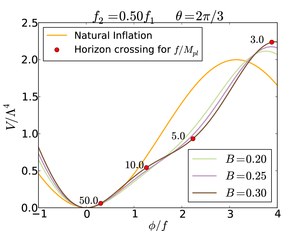
and the constant is fixed so that the inflaton potential at the potential minimum vanishes. We numerically solved the inflation dynamics for three case of , and by varying . The predicted values of as well as the inflaton potential are shown in Fig. 1. The solid (dashed) lines correspond to () e-folds before the end of inflation. Note that, while the lower shaded (red) region shows the region preferred by Planck+WP+highL data allowing the running spectral index to vary, the upper shaded (blue) region is obtained by combining the BICEP2. When the effective neutrino species is varied instead of the running, the allowed region is expected to be shifted to larger values of around unity with . In the right panel, we assume . We also denote several predicted values of for different values of the decay constant as a reference. Interestingly, we can see from the figure that the spectral index close or above unity together with can be realized by multi-natural inflation. Such features will be favored if the tension between BICEP2 and Planck is solved by other sources such as dark radiation, HDM, or non-zero neutrino mass [24].

IV Discussion and Conclusions
We have revisited multi-natural inflation [21] in supergravity for a UV completion. In this model the inflaton potential consists of two or more sinusoidal functions with different height and periodicity. A further UV completion based on a string-inspired framework has been also considered. The moduli stabilization of extra dimensions has to be done to give a sensible string theory in four dimensions. Multi-natural inflation may be realized as a remnant of such moduli stabilization based on various non-perturbative effects.
From an observational point of view, multi-natural inflation is interesting because the existence of small modulations to the inflaton potential, which are necessary to generate a large running spectral index, is a built-in feature. The running spectral index is one way to relax the tension between BICEP2 and Planck. For this to work, we need a mild hierarchy between the two decay constants. On the other hand, the tension could be solved by other sources such as dark radiation88 8 The existence of dark radiation may be ubiquitous in the Large Volume Scenario [55, 56, 57]. , in which case the scalar spectral index close to or even above unity is favored. We have shown that the multi-natural inflation with two sinusoidal functions can realize a wide range of values of that include such cases.
Acknowledgment
We thank Takeshi Kobayashi for useful discussion. This work was supported by Grant-in-Aid for Scientific Research on Innovative Areas (No.24111702, No. 21111006, and No.23104008) [FT], Scientific Research (A) (No. 22244030 and No.21244033) [FT], and JSPS Grant-in-Aid for Young Scientists (B) (No. 24740135 [FT] and No. 25800169 [TH]), and Inoue Foundation for Science. This work was also supported by World Premier International Center Initiative (WPI Program), MEXT, Japan [FT].
References
- [1] P. A. R. Ade et al. [BICEP2 Collaboration], arXiv:1403.3985 [astro-ph.CO].
- [2] A. H. Guth, Phys. Rev. D 23, 347-356 (1981); A. A. Starobinsky, Phys. Lett. B 91 (1980) 99; K. Sato, Mon. Not. Roy. Astron. Soc. 195, 467-479 (1981).
- [3] A. D. Linde, Phys. Lett. B 108 (1982) 389; A. Albrecht and P. J. Steinhardt, Phys. Rev. Lett. 48, 1220 (1982).
- [4] A. D. Linde, Phys. Lett. B 129, 177 (1983).
- [5] K. Freese, J. A. Frieman and A. V. Olinto, Phys. Rev. Lett. 65, 3233 (1990).
- [6] H. Murayama, H. Suzuki, T. Yanagida and J. ’i. Yokoyama, Phys. Rev. Lett. 70, 1912 (1993).
- [7] M. Kawasaki, M. Yamaguchi and T. Yanagida, Phys. Rev. Lett. 85, 3572 (2000) [hep-ph/0004243].
- [8] S. Dimopoulos, S. Kachru, J. McGreevy and J. G. Wacker, JCAP 0808, 003 (2008) [hep-th/0507205].
- [9] R. Kallosh, Lect. Notes Phys. 738, 119 (2008) [hep-th/0702059 [HEP-TH]].
- [10] E. Silverstein, A. Westphal, Phys. Rev. D 78, 106003 (2008) [arXiv:0803.3085 [hep-th]].
- [11] L. McAllister, E. Silverstein, A. Westphal, Phys. Rev. D 82, 046003 (2010) [arXiv:0808.0706 [hep-th]].
- [12] N. Kaloper and L. Sorbo, Phys. Rev. Lett. 102, 121301 (2009) [arXiv:0811.1989 [hep-th]]; N. Kaloper, A. Lawrence and L. Sorbo, JCAP 1103, 023 (2011) [arXiv:1101.0026 [hep-th]].
- [13] F. Takahashi, Phys. Lett. B 693, 140 (2010) [arXiv:1006.2801 [hep-ph]].
- [14] K. Nakayama, F. Takahashi, JCAP 1011, 009 (2010) [arXiv:1008.2956 [hep-ph]]; see also ibid, JCAP 1011, 039 (2010) [arXiv:1009.3399 [hep-ph]].
- [15] K. Nakayama, F. Takahashi and , JCAP 1102, 010 (2011) [arXiv:1008.4457 [hep-ph]];
- [16] K. Harigaya, M. Ibe, K. Schmitz and T. T. Yanagida, Phys. Lett. B 720, 125 (2013) [arXiv:1211.6241 [hep-ph]].
- [17] D. Croon, J. Ellis and N. E. Mavromatos, Physics Letters B 724, , 165 (2013) [arXiv:1303.6253 [astro-ph.CO]].
- [18] K. Nakayama, F. Takahashi and T. T. Yanagida, Phys. Lett. B 725, 111 (2013) [arXiv:1303.7315 [hep-ph]]; JCAP 1308, 038 (2013) [arXiv:1305.5099 [hep-ph]].
- [19] K. Nakayama, F. Takahashi and T. T. Yanagida, Phys. Lett. B 730, 24 (2014) [arXiv:1311.4253 [hep-ph]].
- [20] M. Cicoli, K. Dutta and A. Maharana, arXiv:1401.2579 [hep-th].
- [21] M. Czerny and F. Takahashi, arXiv:1401.5212 [hep-ph].
- [22] M. Czerny, T. Higaki and F. Takahashi, arXiv:1403.0410 [hep-ph].
- [23] K. Nakayama and F. Takahashi, arXiv:1403.4132 [hep-ph].
- [24] E. Giusarma, E. Di Valentino, M. Lattanzi, A. Melchiorri and O. Mena, arXiv:1403.4852 [astro-ph.CO].
- [25] C. R. Contaldi, M. Peloso and L. Sorbo, arXiv:1403.4596 [astro-ph.CO].
- [26] M. Kawasaki and S. Yokoyama, arXiv:1403.5823 [astro-ph.CO].
- [27] V. Miranda, W. Hu and P. Adshead, arXiv:1403.5231 [astro-ph.CO].
- [28] B. Feng and X. Zhang, Phys. Lett. B 570, 145 (2003) [astro-ph/0305020].
- [29] M. Kawasaki and F. Takahashi, Phys. Lett. B 570, 151 (2003) [hep-ph/0305319].
- [30] K. S. Jeong, M. Kawasaki and F. Takahashi, JCAP 1402, 046 (2014) [arXiv:1310.1774 [hep-ph].
- [31] T. Higaki, K. S. Jeong and F. Takahashi, JCAP 1308, 031 (2013) [arXiv:1302.2516 [hep-ph]].
- [32] D. H. Lyth, Phys. Rev. Lett. 78, 1861 (1997) [hep-ph/9606387].
- [33] F. Takahashi, JCAP 1306, 013 (2013) [arXiv:1301.2834, arXiv:1301.2834 [astro-ph.CO]].
- [34] V. Balasubramanian, P. Berglund, J. P. Conlon and F. Quevedo, JHEP 0503, 007 (2005) [hep-th/0502058]; J. P. Conlon, F. Quevedo and K. Suruliz, JHEP 0508, 007 (2005) [hep-th/0505076]; R. Blumenhagen, J. P. Conlon, S. Krippendorf, S. Moster and F. Quevedo, JHEP 0909, 007 (2009) [arXiv:0906.3297 [hep-th]].
- [35] M. Czerny, T. Kobayashi and F. Takahashi, arXiv:1403.4589 [astro-ph.CO].
- [36] T. Kobayashi and F. Takahashi, JCAP 1101, 026 (2011) [arXiv:1011.3988 [astro-ph.CO]].
- [37] H. Shimabukuro, K. Ichiki, S. Inoue and S. Yokoyama, arXiv:1403.1605 [astro-ph.CO].
- [38] O. Lebedev, H. P. Nilles and M. Ratz, Phys. Lett. B 636, 126 (2006) [hep-th/0603047].
- [39] R. Kitano, Phys. Lett. B 641, 203 (2006) [hep-ph/0607090].
- [40] S. Kachru, R. Kallosh, A. D. Linde and S. P. Trivedi, Phys. Rev. D 68, 046005 (2003) [hep-th/0301240].
- [41] K. Choi, A. Falkowski, H. P. Nilles and M. Olechowski, Nucl. Phys. B 718, 113 (2005) [hep-th/0503216].
- [42] E. Dudas, C. Papineau and S. Pokorski, JHEP 0702, 028 (2007) [hep-th/0610297]; H. Abe, T. Higaki, T. Kobayashi and Y. Omura, Phys. Rev. D 75, 025019 (2007) [hep-th/0611024]; R. Kallosh and A. D. Linde, JHEP 0702, 002 (2007) [hep-th/0611183].
- [43] J. P. Conlon, JHEP 0605, 078 (2006) [hep-th/0602233];
- [44] K. Choi and K. S. Jeong, JHEP 0701, 103 (2007) [hep-th/0611279];
- [45] T. Higaki and T. Kobayashi, Phys. Rev. D 84, 045021 (2011) [arXiv:1106.1293 [hep-th]];
- [46] R. Kallosh and A. D. Linde, JHEP 0412, 004 (2004) [hep-th/0411011].
- [47] J. E. Kim, H. P. Nilles and M. Peloso, JCAP 0501, 005 (2005) [hep-ph/0409138].
- [48] R. Blumenhagen, B. Kors, D. Lust and S. Stieberger, Phys. Rept. 445, 1 (2007) [hep-th/0610327].
- [49] M. Grana, Phys. Rept. 423, 91 (2006) [hep-th/0509003]; M. R. Douglas and S. Kachru, Rev. Mod. Phys. 79, 733 (2007) [hep-th/0610102].
- [50] A. Giryavets, S. Kachru, P. K. Tripathy and S. P. Trivedi, JHEP 0404, 003 (2004) [hep-th/0312104].
- [51] G. F. Giudice and A. Strumia, Nucl. Phys. B 858, 63 (2012) [arXiv:1108.6077 [hep-ph]].
- [52] A. Hebecker, A. K. Knochel and T. Weigand, JHEP 1206, 093 (2012) [arXiv:1204.2551 [hep-th]].
- [53] L. E. Ibanez, F. Marchesano, D. Regalado and I. Valenzuela, JHEP 1207, 195 (2012) [arXiv:1206.2655 [hep-ph]].
- [54] A. Hebecker, A. K. Knochel and T. Weigand, Nucl. Phys. B 874, 1 (2013) [arXiv:1304.2767 [hep-th]].
- [55] M. Cicoli, J. P. Conlon and F. Quevedo, Phys. Rev. D 87, 043520 (2013) [arXiv:1208.3562 [hep-ph]]; T. Higaki and F. Takahashi, JHEP 1211, 125 (2012) [arXiv:1208.3563 [hep-ph]]; see also T. Higaki, K. Kamada and F. Takahashi, JHEP 1209, 043 (2012) [arXiv:1207.2771 [hep-ph]];
- [56] T. Higaki, K. Nakayama and F. Takahashi, JHEP 1307, 005 (2013) [arXiv:1304.7987 [hep-ph]];
- [57] S. Angus, arXiv:1403.6473 [hep-ph]; A. Hebecker, P. Mangat, F. Rompineve and L. T. Witkowski, arXiv:1403.6810 [hep-ph].