Statistics for fixed points of the self-power map
Abstract.
The map modulo is related to a variation of the ElGamal digital signature scheme in a similar way to the discrete exponentiation map, but it has received much less study. We explore the number of fixed points of this map by a statistical analysis of experimental data. In particular, the number of fixed points can in many cases be modeled by a binomial distribution. We discuss the many cases where this has been successful, and also the cases where a good model may not yet have been found.
Keywords: self-power map, exponential equation, ElGamal digital signatures, fixed points, random map
2010 Mathematics Subject Classification
11Y99 (primary), 11-04, 11T71, 94A60, 11A07, 11D99 (secondary)1. Introduction and Motivation
The security of the ElGamal digital signature scheme against selective forgery relies on the difficulty of solving the congruence for and , given , , , and but not knowing the discrete logarithm of modulo to the base . (We assume for the moment the security of the hash function .) Similarly, the security of a certain variation of this scheme given in, e.g., [15, Note 11.71], relies on the difficulty of solving
| (1) |
It is generally expected that the best way to solve either of these congruences is to calculate the discrete logarithm of , but this is not known to be true. In particular, another possible option would be to choose arbitrarily and solve the relevant equation for . In the case of (1), this boils down to solving equations of the form . We will refer to these equations as “self-power equations”, and we will call the map modulo the “self-power map”. This map has been studied in various forms in [1, 2, 5, 6, 17, 12, 11, 9, 7, 10, 13]. In this work we will investigate experimentally the number of fixed points of the map, i.e., solutions to
| (2) |
between and . In particular, we would like to know whether the distribution across various primes behaves as we would expect if the self-power map were a “random map”. We do this by creating a model in which values of a map are assumed to occur uniformly randomly except as forced by the structure of the self-power map. We can then predict the distribution of the number of fixed points of this random map and compare it statistically to the actual self-power map. If there is “nonrandom” structure in the self-power map, it may be possible to exploit that structure to break the signature scheme mentioned above or others like it.
Some theoretical work has been done on bounding the possible number of fixed points of the self-power map. If we denote the number of solutions to (2) which fall between and by , then we have:
As far as a lower bound, every has at least as a solution to (2), and at least some primes have only this solution. However, while [13] gives good reason to believe that there are infinitely many such primes, they also prove that these primes are fairly rare:
Theorem 1.2 (Theorem 1 of [13]).
Let be the number of primes less than or equal to as usual. Let denote the set of primes less than or equal to such that . Then
as .
2. Models and Experimental Results
2.1. Heuristics and Normality
Theorem 1.1 gives us a range in which the number of fixed points can lie, but does not say anything about the distribution of the values within that range. As described above, our goal is to create a random model for the self-power map much like was done for the discrete exponential map in [12, 11, 9]. Our first attempt assumed that was normally distributed around the predicted value . (The normality assumption had been successfully used for the discrete exponential map in, e.g., [3], see also [16]. Furthermore, it appeared to be justified by the Central Limit Theorem given the number of primes we were intending to test.)
In order to calculate the variance of , we use the following heuristic, which is related to those in [9, Section 6], and can also be derived from the assumptions in [13, Section 4.1].
Heuristic 1.
The map is a random map in the sense that for all , if are chosen uniformly at random from with , then
As some justification, one can use the methods of [10, Cor. 6.2] to prove the following lemma. This shows that the heuristic holds exactly over the range rather than :
Lemma 2.1.
For all , given fixed and fixed , , such that , then
From there one can prove the following theorem:
Theorem 2.2.
Let be the number of solutions to (2) with and . Then
Proof.
As far as using Heuristic 1, note that it implies that the “experiment” of testing whether is a fixed point behaves as a Bernoulli trial. Let be the number of solutions to (2) with and . Assuming independence of the Bernoulli trials (which is not completely accurate, as we shall see), is distributed as a binomial random variable with trials and success probability . This distribution has mean , as expected, and variance . Summing over gives the predicted mean and variance of .
We tested the hypothesis that was normal with this mean and variance by collecting data for 238 primes from 100,003 to 102,667 and 599 primes from 1,000,003 to 1,007,977. The number of fixed points for each prime was determined using C code originally written by Cloutier [3] and modified by Lindle [14], Hoffman [8], and Friedrichsen-Larson-McDowell [7] Post-processing was done using a Python script written by the first author. The code was run on servers maintained by the Rose-Hulman Computer Science-Software Engineering and Mathematics Departments and took only a few minutes of computational time.
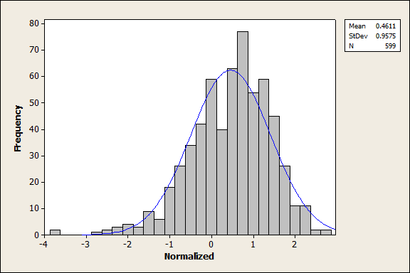
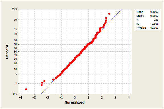
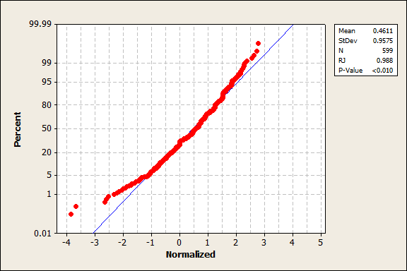
Once the values of were collected, they were normalized to a -statistic by subtracting the predicted mean and dividing by the predicted standard deviation (square root of the variance). The -statistics were grouped separately for the six-digit and seven-digit primes and tested to see if they conformed to the expected standard normal distribution. As you can see in Figures 1 and 2, the distributions appear to be roughly normal to the naked eye, and the standard deviations are close to 1 as expected. The means are closer to 0.5 than the expected 0, and there are a few bars which seem significantly off, but these features could be attributed to certain known properties which appear below in Theorem 2.3. More troubling is the lack of normality revealed by probability plots in Figures 3 and 4. Perfectly normal distributions would lie along the diagonal lines in these figures, and Ryan-Joiner tests confirm that it is very unlikely that is obeying a normal distribution for these primes. In fact there appear to be more primes in the “tails” than expected, that is, a larger than expected number of primes with significantly more or fewer fixed points than expected.

2.2. Binomial Distribution and Goodness of Fit
Some modification of the code by the first author allowed us to collect the values of for the same primes as above, in order to see if particular orders were behaving less “randomly” than others. We excluded certain orders where is known to behave predictably:
Theorem 2.3.
- (1)
for all .
- (2)
for all .
- (3)
for all .
- (4)
To prove this we use the following lemmas:
Corollary 2.5.
Let . The solutions to (2) of order are exactly the elements of which have order .
Proof of Theorem 2.3.
Parts 1 and 2 are clear from the definition. Part 3 is Proposition 6 of [7]. If is a fixed point such that , then Corollary 2.5 implies that . Then Proposition 2 of [7] tells us is a fixed point if and only if is a quadratic residue modulo , which is if and only if or . Combining this with the fact that gives Part 4. ∎
Remark 1.
Note that the behavior of fixed points in safe primes, where is prime, is completely explained by Theorem 2.3.
We collected values of for each prime and each value of other than and . We then attempted to normalize this data, but the resulting -statistics turned out to be too highly clustered and did not resemble normal data. We therefore decided to do a chi-squared goodness-of-fit test on the data. We used the formula for the mass function of a binomial distribution to predict that
Prediction 1.
We chose to use the categories , , , and for our test in order to make sure the categories with large did not get too small. We summed the predictions over and for each of the categories and compared them with the observed numbers of and which fell into each category. The resulting chi-squared statistic was , giving a -value of . Using the common cutoff of for statistical significance, we do not see statistical evidence that our predictions are incorrect.
However, not all values of and fit the predictions equally well. We tested this by sorting in various ways the values of collected for between 100,003 and 102,667, and other than and . After each sort, we calculated the chi-squared statistics and -values for a sliding window of 100 values, with predictions and observations calculated as above. (The size of the window was chosen in order to make sure there were enough data points in the window for the chi-squared test to be valid.)
The strongest evidence of a pattern was seen when the data was sorted by value of , as can be seen in Figure 5. For data randomly generated according to the relevant binomial distributions, -values should be evenly distributed between and . When -values are biased towards 0 it indicates statistically significant divergence from the predicted distributions. In other words, dots on the same (approximate) horizontal line should be evenly distributed between the left- and right-hand sides of the graph. (Note that the value of used to place the dot on the plot is the largest value of in the window of 100 pairs, so some dots would more accurately “belong” to more than one line.) Horizontal lines where the dots are clustered towards the left-hand side indicate statistically significant divergence.
As you can see, the strongest divergence from the predictions occurs with particularly small and particularly large values of . (Since the value of used to place the dot on the plot is the largest value in the window, the effect for small is even larger than it appears in the plot.) We therefore looked for theoretical explanations of these effects.
3. Small and Large Orders
3.1. Small Orders
For we observed that while should occur roughly one-ninth of the time according to Prediction 1, it never occurred at all in our data. A similar but less striking effect was observed for , while for it was which was never observed, despite Prediction 1 saying it should happen over one-quarter of the time. It turns out that there is a significant lack of independence in the fixed points for these orders, as we were able to show.
Theorem 3.1.
- (1)
or for all such that .
- (2)
or for all such that .
- (3)
or for all such that .
Proof.
If , then by Lemma 2.4 the fixed points of order 3 are exactly the elements congruent to 1 modulo 3. In this case there are two elements of order 3, and a direct computation shows that if is one of them, then is the other. Thus the elements of order 3 add up to . So at most one of the elements of order 3 can be a fixed point, proving Part 1. Part 2 is similar except that the elements of order 4 add up to . In Part 3 the elements of order 6 add up to so if one is a fixed point then the other must be also. ∎
The following lemma says that the elements of a given order are approximately uniformly distributed across the residue classes modulo any given .
Lemma 3.2.
Let , , and be positive integers such that and . Let . Let . Then
where is the number of divisors of .
Proof.
The proof is the same as the proof of Equation (7) from [4] with the order equal to instead of . ∎
In particular, we would expect the elements of order to be equally likely to be of any residue class modulo . This leads us to predict that:
Prediction 2.
- (1)
and
- (2)
and
- (3)
and
This is in fact what we observe in the data, as shown in Figure 6. This figure shows the number of primes such that for and , the number of primes for each with , and , and the -value given by a chi-squared test against the distribution predicted above. Once again, we do not see statistical evidence that our predictions are incorrect. (Other small orders do not seem to exhibit this lack of independence in a statistically significant way. For example, fits the distribution of the original model with and fits with .)
3.2. Large Orders
We also observed significant deviation from our predictions in the case of large orders. Recall that Part 4 of Theorem 2.3 used Proposition 2 of [7] to prove that there was at most one fixed point of order . In fact, that Proposition also showed that the fixed point exists if and only if 2 is a quadratic residue modulo . Similarly, if then Corollary 2.5 shows that there are at most two fixed points of order , namely and . Using methods similar to the above we can show that these residue classes will be fixed points when they are cubic residues modulo .
Proposition 3.3.
Let be a prime number equivalent to modulo . The residue class is a fixed point if and only if it is a cubic residue modulo , and similarly for .
Proof.
Note that since , Equation (2) is equivalent to
| (3) |
Then is a fixed point if and only
which by Euler’s Criterion is equivalent to being a cubic residue.
Similarly, if is a fixed point then
But then
also, where the first equivalence is just Fermat’s Little Theorem. So Euler’s Criterion is satisfied again. Conversely, if
then certainly
so is a fixed point.
∎
More simplifications show that and so will be a cubic residue whenever is a cubic residue and both and will be cubic residues when both and are cubic residues. These same methods can be used to show that all numbers of the form where will be fixed points in the self-power map when the number is a -th residue.
This is not quite enough to investigate since not all cubic residues have order equal to . We thus estimate the probability that a given element of , has order equal to exactly . Lemma 3.2 suggests that elements of order occur in in approximately the same proportion that they occur in the whole range , namely . (A more precise statement on the frequency of such that has order would appear to require some variation on Artin’s primitive root conjecture.)
We again use a binomial distribution to predict:
Prediction 3.
- (1)
- (2)
- (3)
If , Corollary 2.5 shows that there are at most three fixed points of order , namely , , and . However, it turns out that they cannot all be fixed points at the same time.
Theorem 3.4.
Let be a prime number equivalent to modulo .
- (1)
If , then .
- (2)
If , then .
Proof.
Suppose . Since and , these two can only be both fixed points of order if . But we know , so if then . On the other hand, if , then we know so neither nor can be . ∎
To make predictions on the probabilities of each number of fixed points, we again use a binomial distribution. If modulo , we keep in mind that the orders of and are dependent and never equal so we can treat them together:
Prediction 4.
- (1)
- (2)
- (3)
If modulo , then we simply have:
Prediction 5.
- (1)
- (2)
Chi-squared tests on the observed data from six-digit primes against the distributions predicted for orders and do not show significant deviation, as shown in Figure 7.
4. Conclusion and Future Work
In practice, it would certainly be possible for a user of the variant ElGamal digital signature scheme to simply make sure is a safe prime, or alternatively arrange for to always be a primitive root. In this way one could avoid the issue of fixed points altogether. However, we feel that it is very likely that a better understanding of the self-power map will help us better understand the security of this and other similar schemes.
We have given some bounds on the number of fixed points of the self-power map and attempted to predict the distribution of the fixed points using a binomial model whose mean is related to these proven bounds. When the order of is moderate, this binomial model is a good predictor according to the data we collected. When the order of is small, in particular when it is 3, 4, or 6, the independence assumption of the binomial model is violated in a significant way. However, we were able to find another model which appears to successfully predict the distribution.
When the order of is or , we once again have a significant deviation from our first binomial model. However, a closer look at the set of possible fixed points in each case leads to another binomial model which appears to be successful. Orders in the range to do not appear to be showing significant deviation from the original model. However, the sliding window chi-squared test shows evidence of possible divergence from the predictions in the neighborhood of , as can be seen in Figure 5 about three-quarters of the way from the “Order 1000” horizontal line to the “Order 10000” line. It is not clear yet whether this is a true problem with the model, or just a “random” consequence of the particular primes that we picked. Further investigation of these orders would appear to be the first item to be considered in future work.
Another very important item of future work would be to consider two-cycles, namely solutions to the equations
| (4) |
or more generally -cycles. Some data has been collected for these larger cycles but the binomial distribution has not yet been calculated or checked. The paper [7] also examined other graph-theoretic statistics of the functional graphs created by the self-power map, especially the number of components. This was also found to obey a non-normal distribution and one would like to explore how that distribution is related to the one found here for fixed points.
Acknowledgements
Many thanks to Richard Layton for the design and production of Figures 6 and 7. We also thank the Rose-Hulman Computer Science-Software Engineering and Mathematics Departments for the use of their computers.
References
- [1] (2013) The self power map and its image modulo a prime. PhD Thesis, University of Toronto. External Links: Link Cited by: §1.
- [2] (2011) On the number of solutions of exponential congruences. Acta Arithmetica 148 (1), pp. 93–103. External Links: Link, Document Cited by: Theorem 1.1, §1.
- [3] (2010) Mapping the discrete logarithm. Involve, a Journal of Mathematics 3 (2), pp. 197–213. External Links: ISSN 1944-4176, Link, Document Cited by: §2.1, §2.1.
- [4] (1999) An exponential congruence with solutions in primitive roots. Rev. Roumaine Math. Pures Appl. 44 (1), pp. 15–22. External Links: ISSN 0035-3965 Cited by: §3.1.
- [5] (1966) On a new problem in number theory. The American Mathematical Monthly 73 (4), pp. 355–357. Cited by: §1.
- [6] (1969) On residues of . The American Mathematical Monthly 76 (9), pp. 1028–1029. Cited by: §1.
- [7] (2010) Structure and statistics of the Self-Power map. Rose-Hulman Undergraduate Mathematics Journal 11 (2). Cited by: §1, §2.1, §2.2, Lemma 2.4, §3.2, §4.
- [8] (2009) Statistical investigation of structure in the discrete logarithm. Rose-Hulman Undergraduate Mathematics Journal 10 (2). External Links: Link Cited by: §2.1.
- [9] (2006) Some heuristics and results for small cycles of the discrete logarithm. Mathematics of Computation 75 (253), pp. 419–449. External Links: ISSN 0025-5718 Cited by: §1, §2.1, §2.1.
- [10] (2012) Counting fixed points, Two-Cycles, and collisions of the discrete exponential function using -adic methods. Journal of the Australian Mathematical Society 92, pp. 163–178. Cited by: §1, §2.1.
- [11] (2002) Addenda/corrigenda: fixed points and two-cycles of the discrete logarithm. Note: Unpublished, available at http://xxx.lanl.gov/abs/math.NT/0208028 External Links: arXiv:math/020802 [math.NT] Cited by: §1, §2.1.
- [12] (2002) Fixed points and two-cycles of the discrete logarithm. In Algorithmic number theory (ANTS 2002), C. Fieker and D. R. Kohel (Eds.), LNCS, pp. 405–415. External Links: Link Cited by: §1, §2.1.
- [13] (2015) On the fixed points of the map modulo a prime. Mathematical Research Letters 22, pp. 141–168. External Links: Document Cited by: Theorem 1.1, Theorem 1.2, §1, §1, §2.1.
- [14] (2008) A statistical look at maps of the discrete logarithm. Senior Thesis, Rose-Hulman Institute of Technology. Cited by: §2.1.
- [15] (1996) Handbook of applied cryptography. CRC. External Links: ISBN 0849385237, Link Cited by: §1.
- [16] (2008) Poster abstracts from the eighth algorithmic number theory symposium, ANTS-8. ACM Communications in Computer Algebra 42 (2), pp. 48–66. External Links: Link Cited by: §2.1.
- [17] (1981) The residues of modulo . Fibonacci Quarterly 19 (2), pp. 110–117. Cited by: §1, §2.1.