Parameter estimation of social forces in crowd dynamics models via a probabilistic method
Abstract.
Focusing on a specific crowd dynamics situation, including real life experiments and measurements, our paper targets a twofold aim: (1) we present a Bayesian probabilistic method to estimate the value and the uncertainty (in the form of a probability density function) of parameters in crowd dynamic models from the experimental data; and (2) we introduce a fitness measure for the models to classify a couple of model structures (forces) according to their fitness to the experimental data, preparing the stage for a more general model-selection and validation strategy inspired by probabilistic data analysis. Finally, we review the essential aspects of our experimental setup and measurement technique.
Key words and phrases:
Crowd dynamics, parameter estimation, Bayes theorem, models classification, data analysis.1991 Mathematics Subject Classification
Primary: 35R30, 91D10; Secondary: 62F15, 91C99.Alessandro Corbetta
CASA- Centre for Analysis, Scientific computing and Applications,
Department of Mathematics and Computer Science, Eindhoven University of Technology,
P.O. Box 513, 5600 MB Eindhoven, The Netherlands,
Department of Structural, Geotechnical and Building Engineering,
Politecnico di Torino, Corso Duca degli Abruzzi 24, 10126 Torino, Italy
Adrian Muntean
CASA- Centre for Analysis, Scientific computing and Applications,
ICMS - Institute for Complex Molecular Systems
Department of Mathematics and Computer Science, Eindhoven University of Technology,
P.O. Box 513, 5600 MB Eindhoven, The Netherlands,
Federico Toschi
Department of Physics and Department of Mathematics and Computer Science,
Eindhoven University of Technology, P.O. Box 513, 5600 MB Eindhoven, The Netherlands,
CNR-IAC, Via dei Taurini 19, 00185 Rome, Italy,
Kiamars Vafayi
CASA- Centre for Analysis, Scientific computing and Applications,
Department of Mathematics and Computer Science, Eindhoven University of Technology,
P.O. Box 513, 5600 MB Eindhoven, The Netherlands,
1. Introduction
1.1. Background
Crowd models are powerful tools to explore the complex dynamics which characterizes the motion of pedestrians, cf. e.g. the overview [27] and references cited therein. Understanding how crowds move and eventually being able to predict their behavior under given (possibly extreme) conditions becomes an increasingly important matter for our society. Reliable mathematical models for crowds would be of great benefit, for instance, to increase pedestrian comfort (ensuring a regular flow motion at acceptable densities), security (evacuation assessments) and structural serviceability (crowd-structure interaction), in particular if the theoretical information/forecast is in real-time agreement with the actual crowd behavior.
Aiming at quantitative models, a proper assessment of the uncertainty is needed given experimental data (e.g., in the form of crowd recordings) together with a model or a collection of models. This paper treats a basic crowd scenario: pedestrians crossing an U-shaped landing (corridor) in a defined direction. In particular, the questions we consider here relate to a low density regime, in which pedestrians can be considered as moving alone, being just influenced by their desires as well as the geometry of the (built) environment in their surroundings (“rarefied gas” regime). We explicitly wonder (in a quantitative sense specified afterwards): do pedestrians interact with walls? How does the presence of walls affect the pedestrian motion? Are walls purely repulsive, or could they be attractive?
To address these (and related) questions, we made many video recordings of the landing considered (see Appendix A) and took as test models 7 different evolution equations describing the pedestrian-wall interaction.
1.2. Simple crowd models. Ensembles
Since the movement of pedestrians is to a large extent non-deterministic, any model that describes the detailed motion of pedestrians requires the introduction of some elements of noise. To address this issue, one may choose to describe the dynamics from a “coarse grained” point of view, hence either at the mesoscopic scale or at the macroscopic scale. For instance, when a macroscopic level of description is used, a balance equation for the density of pedestrians (possibly supported by balance of momentum, see e.g. [8] for details on balance laws) models the evolution of the crowd, while the detailed microscopic behaviors are averaged out. In principle, the latter equations can be derived directly from the microscopic equations, although a problem remains: microscopic models for crowd dynamics (see, for instance, the social force model proposed by Helbing and Molnar [15]) describe the detailed motion of pedestrians, but to which extent the microscopic details are relevant to capture the intrinsic crowd patterns at larger scales and what is the role of noise and uncertainty? In other words, which details of the microscopic information are necessary to capture the behavior of the crowd?
Usually, in an attempt to keep into account the observed non-deterministic behavior of the crowds, noise is added to deterministic models turning them into Langevin-like equations for the so-called active Brownian particles (see e.g. [26, 27]) or in measure-valued evolutions (see e.g. [1, 13, 2]).
Since we cannot describe deterministically the motion of pedestrians, we opt for a different strategy. We choose to construct a probabilistic ensemble of pedestrians (referred here as the ensemble11 1 By “ensemble” we understand a collection of the copies of a system distributed according to a probability distribution function (pdf).) whose properties can be directly deduced in a quantitative manner on the basis of experimental observations.
We construct such crowd ensemble by the means of a connection to simple evolution models, which can be cast in the form of a potential of interaction of pedestrians with obstacles or amongst themselves together via Newtonian dynamics. The potential or force in the model is characterized by a set of parameters, whose statistical properties can be obtained by comparing the model with well-controlled experimental data. Thus the model and the probability distribution of the model parameters (inferred from data) define our crowd ensemble. In this way we cast the force estimation problem into a well defined procedure of probabilistic data analysis, very much inspired by [30, 29]. A related approach for traffic-flow models is mentioned in [16] and references therein.
1.3. Aim of the paper
We focus our attention on the effects of walls (obstacles) on pedestrian motion for a specific crowd dynamics scenario (extensively described in Section 1.4 from a qualitative point of view, and in the Appendix A from a technical point of view). Once the effect of walls is understood, considering pedestrian-pedestrian interactions in the same scenario is expected to be easier.
Note that even standard crowd dynamics situations are actually rather complex, in particular, the following aspects among others need to be considered carefully:
- (i)
the motion of pedestrian is complex and influenced by many sources, among others: desires/aims, interaction with geometry and interaction with neighboring peers;
- (ii)
the effects of these interaction appears simultaneously and in an entangled way.
To attempt to disclose the cause-effect relations in this complex motion, we choose a step by step approach; therefore, we opt to look exclusively at situations in which the interaction among pedestrians is absent and the motion is fully regulated by own desires and neighboring geometry. As a clear consequence, this study sets a possible stage for the analysis of pedestrian-pedestrian interactions which is inevitably perturbed by the effects mentioned at (i) and (ii). To make the complete dynamics approachable, the hypothesis of linear superposition of effects has to be made.
In social-force models [15, 10, 25, 32, 4] (for overviews on the matter see, e.g., [12, 27]), pedestrians move according to a Newtonian dynamics; in particular, in the absence of neighboring peers, the force acting on a single particle can be expressed as:
| (1) |
where
- •
is a force which keeps into account the desires of the pedestrians in terms of the direction he/she is willing to follow. Usually, this term induces a relaxation of the velocity of the pedestrian towards a background desired velocity field . The desired velocity field usually drives the pedestrian all over the domain toward a given “desired” target. In formulas, this term reads as , where is a characteristic relaxation time.
- •
describes the interactions pedestrians have with walls. This term doesn’t just model the impenetrability of the latter, rather it is aimed at taking into account the will of pedestrians to maintain a certain distance from walls.
Structure and parameters dependence of and shall be assumed. In the following, we suppose to be parametrized by its magnitude (the desired speed ), whilst its direction is kept as a model feature.
On the other hand, is assumed to be a sum of forces pointing outwards every wall in the particle proximity, i.e.
One usually supposes that every contribution has a fixed functional form which depends on the distance between the pedestrian and the wall, and is parametrized by a set of parameters . Note, however, that different, more general, forms of can be chosen; see e.g. [17].
1.4. Experimental data
The kinematic data referring to trajectories of pedestrians (positions, velocities, accelerations) walking through a rectangular landing (see Figure 1. Consider Appendix A for details), are acquired via an over head recording camera. Due to the geometry of the setting, trajectories of pedestrians tend to bend slightly as the landing is crossed. This is a consequence of the presence of degree turns at the entrance and at the exit of the landing.
In the following, since we focus our attention on the walls-pedestrian interaction, we consider only data concerning a single pedestrian (i.e. appearing alone in the camera field of view) and going in a specific direction (specifically, from left to the right) are considered. In other words, all data referring to situations in which more than one pedestrian are present at a time are not taken into consideration.


The final measured data consists of a set of pedestrian trajectories ()
Every trajectory is a set of recorded points in the -dimensional space-time of the landing (i.e., a given pedestrian having trajectory has spatial position at time instant ). In formulas, we describe a trajectory like
| (2) |
where is the number of points in the considered trajectory.
Remark 1.
Looking back at the considered model parameters (i.e., the desired speed and the wall force parameters, ), we observe that is a parameter specific of the trajectories, i.e. to every trajectory it corresponds a specific value that needs to be estimated. In contrast, one can think of as a set of global parameters, in the sense that they are shared between all trajectories. This would suggest the use of a two-steps optimization procedure; see Section 2.4. In this paper, we decide to treat all parameters in the same way, and thus we postpone the two-steps optimization idea for a later approach.
1.5. Structure of the paper
The paper is organized as follows: Section 2 contains the working methodology which is based on probability estimates guided by Bayes theorem; in Section 3 we point out how Bayes theorem can be used for model selection. The main result of this paper is presented in Section 4: following the described working methodology, parameters of a number of simple wall force models for our crowd scenario are estimated. Moreover, on this basis, models are compared quantitatively and qualitatively. Section 5 discusses the obtained results. Finally, the measurement technique and the collected experimental data are described in Appendix A.
2. Probabilistic data analysis of crowd ensembles
In this section, we introduce the methodology behind the probabilistic data analysis used here. For more details, we refer the reader to the introductory guide by Skilling [30] or to the mathematical background presented by Sivia in [29].
2.1. Probability estimates. Bayes theorem
We denote all the measured data by and all prior information by . In other words, while encloses all the information acquired in the measurement process, includes the assumptions made on model and thus on the type of dynamics.
Our goal is to identify the parameters for a considered set of pedestrian models () for the considered scenario. This task can be performed by estimating the posterior probability law
which describes the probability associated to the parameters of a considered model being conditioned on data and all prior information . Such probability law can be either peaked around a given maximum value, which does correspond to the solution of the estimation problem, or can be dispersed. In such case the mean value and the standard deviation of the law can be used as a fair representation of the full distribution.
By means of Bayes theorem (see e.g. [7, 6, 20]), the posterior probability can be related to other probabilities of easier computation (or even known already). The theorem reads as
| (3) |
The probabilities involved in the l.h.s are respectively
- •
the likelihood function ;
- •
the prior probability ;
- •
the data evidence .
In the following subsections such probabilities are extensively used and details regarding their computations are given. It is worth to notice that, since the data is assumed as given, the data evidence plays the role of a mere normalization constant and, as a consequence, we can write
| (4) |
to stress the fact that the quantities playing a significant role in parameter estimation are just the likelihood function and the prior probability.
2.2. Likelihood function. Misfit norm(s)
The likelihood function measures how well the model with the given parameters fits the data. We distinguish between four different schemes to compare data and models:
- (i)
positions in trajectory data versus positions predicted in the model;
- (ii)
velocities obtained from data versus velocities as calculated from the model;
- (iii)
acceleration deducted from data versus acceleration in the model;
- (iv)
a combination of the previous three.
It is worth to remark that the third scheme has the advantage of not requiring the computation of the full trajectories generated by the model. On the other hand, acceleration data are usually more noisy, as a consequence of the double time differentiation of pedestrian trajectories (which is never exempt from noise).
The likelihood function can be obtained from the Principle of Maximum Entropy (MaxEnt) once the kind of noise in the data is assumed, see [29] for details. In particular, assuming Gaussian noise, the likelihood function results in
| (5) |
where is the acceleration in the trajectory data, at sample , and is the acceleration provided by the model with parameters and at the same point. According to the adopted notation, is the error estimation, or standard deviation, for the experimental acceleration .
We consider the likelihood function for two different assumptions on the noise in the data: (i) Gaussian noise and (ii) Exponential noise. Different assumptions on the noise may be made22 2 Note that in the Bayesian framework the noise is part of the model.. The choices (i) and (ii) seem to be more common in literature. In this paper, we decide to employ (i) and to leave for further investigations the structure of the noise in our data (see [5]).
2.2.1. Gaussian noise
The misfit function is defined such that
or
Therefore, for the case of Gaussian noise in the data, we have the norm for the “distance” between the model and data;
Since the logarithm is a monotonically increasing function, finding the maximum of is equivalent to finding a minimum for . It becomes more simplified if are equal to ,
or more reasonably since we would intuitively expect that the error estimate be proportional to the data and define a new misfit norm by dividing the previous one by ;
Remark 2.
Since we do not study explicitly the absolute magnitude of the noise, we take everywhere in the paper to be .
This form of has the interesting property that if , i.e., if the model misses the data by a (small) fraction of of the error estimate, then we have
2.2.2. Exponential noise
The exponential noise in the data corresponds to
therefore the misfit in this case will be the norm
Again if we assume and divide by we obtain
A similar calculation as the one we did for Gaussian noise for the deviation , yields
The exponential distribution is less centrally distributed than a Gaussian. Consequently, the norm is more robust and it is expected to fit better data that contains a number of “wildly” distributed points.
With our choice of the misfit functions , we are de facto pushing forward an empirical probability measure (defined by the data), from the parameter space onto the real line. This allows us to compare in a natural fashion different models.
2.3. Prior probability
2.3.1. Backgorund
The prior probability encodes our prior state of knowledge on the parameters, before taking into account the acquired data . For most practical purposes we can suppose that it is a constant over the range of parameters that we consider acceptable. More precisely we can use the symmetry group transformations and/or the principle of maximum entropy to assign the prior probabilities. From translation symmetry arguments, it turns out that for position parameters, like coordinates, a uniform prior distribution over the expected range is the optimal choice. For scale parameters, the right prior is the Jeffreys distribution , which is a consequence of scale invariance symmetry [20, 18, 19]. As long as the data is of good quality and the range of parameters is chosen well, one expects that the effect of the likelihood function dominates, and the posterior probability is less sensitive to the exact choice of the prior probability.
2.3.2. Law of large numbers
Since the number of trajectories measured can be arbitrarily large, we expect that the law of large numbers applies and that one can use an optimization procedure on each single trajectories separately and then employ the resulting histogram to estimated the parameters as the probability distribution for the value of the parameters. Thus having access to a large number of trajectories simplifies the estimation scheme.
2.4. Two-steps optimization
As mentioned in Remark 1, the experimental technique and setup indicate that there is an intrinsic difference between the parameters and , the former being trajectory dependent and the later being global. One way to take this into account is to estimate firstly the parameters for each trajectory, in particular , obtaining As the second step, one can afterwards use the data for globally estimating and calculating the global fitness of the model to data. We do not follow this approach here, rather we treat all parameters equally.
2.5. Simulated annealing
The parameter space is in general multidimensional, and posterior probability is likely to be multi-modal, where the probability maximums (or the minimum of the misfit norm) are generally not analytically solvable. One can use the simulated annealing method [21] to tackle this problem; in analogy with thermodynamics, one supposes that the misfit norm is an energy function and uses the Metropolis Monte Carlo algorithm [23] to sample the points in parameter space according to the Boltzmann-Gibbs distribution at a given temperature, :
Clearly by setting we get the same distribution as the desired likelihood probability. The basic idea of simulated annealing is to start with and then reduce the temperature dynamically until . In this way, starting from a more “energetic” point, it is more likely to overcome the local minimum traps of the misfit function, and reach the most significant parts around the global minimum. Afterwards we will continue the sampling with to obtain the points in parameter space distributed according to the posterior. In order to achieve good convergence, it might be necessary to repeat the whole annealing procedure several times and by starting from different random initial points. The resulting distribution can be used to obtain the marginal probability distribution of for example ;
which can be directly plotted or used to calculate the average and the standard deviation for the parameter;
In the framework of this paper, using many trajectories as data, we perform the per-trajectory optimization approach mentioned in Section 2.3.2 and we thus do not require the simulated annealing approach.
3. Selection and hierarchy of models
3.1. Background
Suppose we have two models and . In such case, we can apply the Bayes theorem to obtain
and, similarly for . Therefore, we have
In general, the two models will have different set of parameters, and , respectively. We have for the data and assuming model that
hence
indicates our prior probability for the model . The integrals over the likelihood function can be calculated with the same stochastic procedure as explained in the section for simulated annealing. We see now that the parameters priors play a role, therefore it is important to make sure they are assigned properly, especially when the two models are nearly identical. We take here but, in principle, this ratio does not need to be one and it can therefore be used for the updating procedures provided previous information are available.
3.2. Law of large numbers
As in the previous section, we use again the fact that we are in a law of large numbers regime and, after the optimization procedure on each single trajectory separately, we use the resulting histogram of the minimum value of the misfit function as the criteria for the model selection. If only one number is required to compare the models, it will be then the average of
| (6) |
in such histograms, for each model, the smaller values are an indication that the model fits better to the data.

4. Estimating wall forces
4.1. Choice of models
We consider different simple crowd models which we denote by the symbols , respectively. We apply the probabilistic parameter estimation technique described in Section 2 - Section 3, together with our experimental test scenario described in Appendix A.
The chosen models aim at reproducing the basic aspects of the pedestrian motion for individuals going from the left hand side to the right hand side of the landing. As previously mentioned (see also Figure 1 (right)), pedestrian trajectories are slightly bending as a consequence of the landing shape.
feature different levels of complexity as more and more phenomenological aspects are introduced. In the simplest case, a rightward directed homogeneous velocity field is considered. Hence, terms to take into account the wall forces and also to keep track of the shape of the corridor (e.g. via the desired velocity) are added.
More precisely, the models are:
- :
An homogeneous desired velocity field parallel to the span-wise walls is adopted. The repulsion force of the walls is neglected. The relaxation time is hereby adopted as fixed and, according to [15], the value is chosen. As a consequence, the parameter to estimate is the desired speed , i.e. ; see Figure 2 (top).
- :
An homogeneous velocity field analogous to the one in is chosen, however the relaxation time is also treated as a parameter to be estimated, i.e. .
-
These models are similar - respectively - to and , and they differ from the latter as the desired velocity field is such that at every point the desired velocity vector is directed towards the exit point, i.e. and ; see Figure 2 (middle).
- :
This model features exclusively the wall force and no relaxation toward a desired velocity field. This force is directed radially in any point toward the center of the “lower” wall.
More precisely, the force at a point is given by
where is the magnitude of the force and is a unit vector field pointing towards . Moreover, we assume that
where and are parameters to be estimated and is the distance of the point to the center of the lower wall, i.e. .
- :
This is a particular case of where we suppose that the force magnitude is constant, i.e.
Here is the parameter to be estimated, in other words, .
- :
This is similar to but, in addition to the force, a desired velocity is also taken into account. This desired velocity field is chosen to be similar to one in the models and , pointing towards the exit. As in , s, i.e. .
4.2. Optimization method
We use the norm for the misfit function (corresponding to the choice of Gaussian noise) and a “global” brute-force-based optimization procedure to find the best fitting parameters per trajectory. A priori knowledge on the parameters range is assumed and this defines a box in the parameters space. The box has been evenly sampled and the cost function has been evaluated. A gradient descent approach is then applied on the sample of minimum cost used to refine the result.
In Figure 3, we compare the models based on the histogram distribution of the misfit function. In Figures 4 and 5, empirical distributions of the value of the parameters are histogrammed. In Table 1 the average value of the parameters and the misfit norms calculated from the histograms are presented.


4.3. First observations
Looking at the results of the estimation method, shown in Figure 3, we observe that in the sense of accordance with the data33 3 As mentioned before, the property of having the least amount of , or, in other words; the more the distribution of gravitates towards , the better the fit. the two best performing models are the force only models, that is and , then followed by .
The wide reduction in terms of in compared to shows the importance of having a good44 4 In this context, by “good” we mean small misfit or large likelihood. desired velocity field, and that more complicated fields might reduce even further. However, it is still more than for , even though uses a quite simple force field.
Comparing the outcome for models and (or similarly for models and ), we notice that introducing the extra parameter for the relaxation time decreases , thus making a better fit to the data. However it has a negligible effect on the magnitude of the desired velocity. The average , on the other hand, is rather dependent on the desired velocity field, as it can be seen from a comparison of models and , but again the average magnitude of the desired velocity is not very sensitive to the choice of the field and in fact varies very little across the models , , , and . The estimated desired speed shows agreeing values (see the histograms of in Figures 4 and 5, and its average values in Table 1) which, furthermore, are slightly overestimating the actual pedestrian velocities measured () consistent with the fact that they define a comfortable target velocity the pedestrians aim at achieving.
We found considerable correlations between the values of and in the models and . This indicates that the data that we have is not able to estimate these two parameters separately very well, but their sum can be rather well estimated, which is approximately (given that in and is small) what is being done in , where the histogram for is more sharply peaked than the histogram for either or in the models and .
| Model | ||||||
|---|---|---|---|---|---|---|
| - | - | - | - | |||
| - | - | - | ||||
| - | - | - | - | |||
| - | - | - | ||||
| - | - | |||||
| - | - | - | - | |||
| - |
5. Discussion
Focusing on a specific pedestrian dynamics scenario, we presented a procedure for estimating models parameters for pedestrian movement based on cameras real life measurements. Basing the method on its Bayesian foundations, we indicated how having access to a large number of measurements simplifies and improves the parameter estimation and the models selection procedures.
The desired velocity and external force acting on pedestrians are two different modeling routes and ingredients, used sometimes separately, and sometimes in combinations. For instance, in the social force model both ingredients are usually present. In the simple landing setup studied in this paper, we found that in case that we use simple models based on force or desired velocity fields, the force-only models do a significantly better job to match the data. The force-only models apparently outperform also models that combine force and desired velocities. This is presumably due to the fact that the slight increased complexity of the model is not necessarily producing better fit to the data in general. The outcome of such increase in models complexity is nontrivial.
Possible extensions of this work can go in multiple directions: for instance, one definitely needs to study other geometries and experimental setups as well as more detailed models allowing for instance the interplay between pedestrian(s)-wall vs. pedestrian-pedestrian interaction. Last but not least, we expect that from the experimental measurements much can be learned on the time and space structure of the correlations in the pedestrian flow (to be followed by us in [5]).
Finally, it worths noting that the approach presented here is not exclusively meant for crowd dynamics applications. The parameter identification procedure can be exploited in a large variety of settings ranging from the tracking of cells motion in biological flows, the motion of colloidal suspensions, the detection of localization patterns of stress-driven defects in materials.
Appendix A Experimental setup
We provide hereby fundamental information on the experimental setup and data used in this paper.
A.1. Lagrangian measurement of pedestrian dynamics
The experimental data considered in this paper, which have been used as a reference to tune and to compare pedestrian models, have been collected during a months-long experimental campaign.
Heavily trafficked landing (see Figure 6), which connects the canteen to the dining area of the MetaForum building at Eindhoven University of Technology, has been recorded on full-time (24/7) basis. These recordings allowed us to gather the statistics concerning pedestrian trajectories that we considered throughout this manuscript.

It is important to highlight that our data do not refer to pedestrians instructed a-priori to cross the landing (as common in many “laboratory” crowd experiments); rather, they refer to the actual, unbiased, “field” measurement of pedestrian traffic.
Following an approach similar to the one already introduced by Seer et al. [28], we performed recordings by employing a standard commercial Kinect™ sensor by Microsoft Corp. [24] that allows reliable acquisition of pedestrian positions.
The Kinect™ sensor is equipped with a special camera designed to enhance natural interaction, i.e. an interaction with computers and the gaming consoles (Microsoft Xbox 360™) based on movements. In particular, in addition to an ordinary camera, the Kinect™ is able to perform hardware measurements of the depth map of the observed scene. The depth map is a two dimensional grey-scale map which associates to every recorded pixel an intensity proportional to its distance from the camera plane (see Figure 7). In our experiments, in order to track pedestrians, we did not acquire any recordings from the standard camera, rather we relied totally on the depth map measurements.

As typically done in literature (cf. e.g. [14, 3, 22]) when one is concerned with the measurement of pedestrian trajectories, it is often favorable to record the top view of the scene. From the top view phenomena like partial body exposure to the camera or mutual hiding, are absent. The problem of constructing pedestrian trajectories can be solved via identification and tracking of heads. Although the heads are always exposed to a top-viewing camera, performing their automatic tracking without additional hypothesis, e.g. on the clothing of pedestrian, can be hard. As pointed out in [28], the depth map associated to the top view of a given scene can be fruitfully used to detect heads. Heuristically speaking, the objects which are closest to the camera generate the local minima in the depth map: such objects, modulo a background subtraction, are most likely to be heads.
To generate pedestrian trajectories, “raw” depth maps were first processed to extract heads positions in each frame; then, well-established particle tracking algorithms (developed for Particle Tracking Velocimetry) were used to generate tracks.
A.2. The algorithm
We report hereby the overall algorithmic procedure. Note that some of the first steps coincide with those explained in [28].
Let be the depth map recorded by Kinect™ (VGA resolution ) at time instant at position , i.e.
| (7) |
where is a point in the VGA frame.
- (1)
Background subtraction. In the recorded picture, and hence in the depth maps, a common background is expected.
To detect pedestrians, the foreground must be first isolated. Let be a depth map of the background (possibly built after suitable averages of empty backgrounds), the foreground associated to a depth map is obtained through the thresholding
where is a given (small) threshold, and if proposition holds true, , otherwise.
- (2)
Height thresholding. A second thresholding operation is performed to eliminate objects which, although part of the foreground, are too small to be pedestrians, i.e.
- (3)
Generation of a sparse depth map. For computational reasons, the foreground of the thresholded depth map is random sampled generating a sparse depth map of samples
where every pair satisfies , i.e. the selected sample owns to the foreground and, likely, to a pedestrian.
- (4)
Sparse samples clusterization and pedestrian detection. In order to identify and isolate pedestrians, sparse samples are agglomerated in macro-samples which likely are in correspondence with pedestrians themselves.
The agglomeration is performed via a hierarchical clustering based on the geometrical distance between points, in particular, a complete linkage clustering algorithm is used [11]. Heuristically speaking, the sparse samples get agglomerated in a binary fashion forming larger and larger macro-samples. Ideally, macro-samples whose mutual distance is larger than the scale length of the human body (e.g., average distance between the shoulders) do correspond to individuals.
The iterative agglomeration procedure merges macro-samples on the basis of their distance starting from the closest pairs. In particular, given two macro-samples and , the metric used satisfies
where is the ordinary euclidean distance on the plane.
The agglomeration procedure can be described as reported below. It is worth to remark that has computational complexity , while optimal computational complexity can be reached [11].
Data: Set of all the samples (as macro-samples):while doend whileThe procedure, which iteratively builds the super-sample , can be visualized via a dendrogram (see Figure 8).
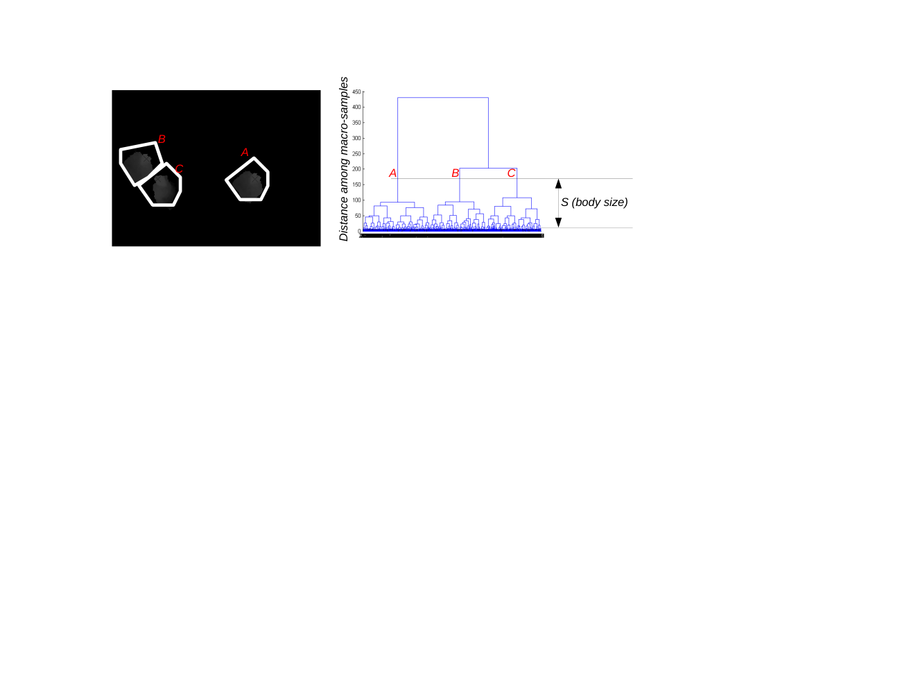
Figure 8. Left: depth map in which three pedestrians have been separated; on the right: cut dendrogram at height , three macro-samples are present. To conclude, we observe that if the agglomeration procedure is truncated at a step such that
then the super-samples in feature a mutual distance larger than ; as such, they are associated with pedestrians.
- (5)
Head position estimation. Given pedestrian identified by the cluster , for some , (being the total number of pedestrians present in frame ), we consider as head the set of samples whose depth is smaller than a given percentile (usually ) of the depth distribution of ,
The head position is then estimated considering the centroid of the set, in formulas
- (6)
Linking positions across the frames. An estimate of the heads position across the frames has been given. In order to approximate the pedestrian trajectories, heads positions must hence be tracked.
The problem of tracking time-sampled particle positions has been studied in several fields, in particular, it is central in Experimental Fluid Dynamics when a Lagrangian approach to flows is pursued. Following standard approaches in experimental Particle Tracking Velocimetry (PTV), and especially via OpenPTV [33, 31], Pedestrian trajectories are generated. In particular, sequences in the form of Equation (2) are obtained.
- (7)
Estimation of kinematic observables associated to trajectories. Once the trajectories are known in their sampled form, kinematic observables such as velocities and accelerations must be estimated. Since the head estimation procedure is not exempt of measurement noise, and a certain degree of regularity in trajectories is expected, a smoothing spline (with smoothing parameter ) is used [9] (See Figure 9 for an example of some of the final trajectories).

Figure 9. A sample selection of 20 pedestrian trajectories in the final data.
After such procedure, the set of trajectories including relative velocities and accelerations is deducted.
Acknowledgments
We would like to thank Ad Holten and Gerald Oerlemans for the help with the installation of the Kinect™ sensor in the MetaForum building at TU/e. We thank Dr. Alex Liberzon (Tel Aviv, Israel) for his precious help with the adaption of the Particle Tracking software to our project. We acknowledge the hosting of Lorentz Center (Leiden, The Netherlands), where, during the workshop “Modeling with Measures”, a part of this paper has been written. KV would like to acknowledge the support of NWO VICI grant 639.033.008.
References
- [1] H. T. Banks and W. C. Thompson, Least squares estimation of probability measures in the Prohorov metric framework, Center for Research in Scientific Computation Tech Rep, CRSC-TR12-21, North Carolina State University, Raleigh, NC.
- [2] N. Bellomo, B. Piccoli and A. Tosin, Modeling crowd dynamics from a complex system viewpoint, Mathematical Models and Methods in Applied Sciences, 22 (2012), 1230004.
- [3] M. Boltes and A. Seyfried, Collecting pedestrian trajectories, Neurocomputing, 100 (2013), 127–133.
- [4] L. Bruno and A. Corbetta, Multiscale probabilistic evaluation of the footbridge crowding. part 2: Crossing pedestrian position, in Proceedings of Eurodyn 2014, Accepted, 2014.
- [5] A. Corbetta, A. Muntean, F. Toschi and K. Vafayi, Structural identification of interaction terms in a Langevin-like model for crowd dynamics, in preparation, 2014.
- [6] R. T. Cox, Probability, Frequency and Reasonable Expectation, American Journal of Physics, 14 (1946), 1–13.
- [7] R. Cox, Algebra of Probable Inference, Algebra of Probable Inference, Johns Hopkins University Press, 1961.
- [8] C. M. Dafermos, Hyperbolic Conservation Laws in Continuum Physics, Grundlehren der mathematischen Wissenschaften, Springer, Berlin, New York, 2000.
- [9] C. De Boor, A Practical Guide to Splines, vol. 27, Springer-Verlag, New York, 1978.
- [10] P. Degond, C. Appert-Rolland, M. Moussaid, J. Pettre and G. Theraulaz, A hierarchy of heuristic-based models of crowd dynamics, Journal of Statistical Physics, 152 (2013), 1033–1068.
- [11] R. O. Duda, P. E. Hart and D. G. Stork, Pattern Classification, John Wiley & Sons, 2012.
- [12] D. C. Duives, W. Daamen and S. P. Hoogendoorn, State-of-the-art crowd motion simulation models, Transportation Research Part C: Emerging Technologies, 37 (2013), 193 – 209.
- [13] J. Evers, S. C. Hille and A. Muntean, Well-posedness and approximation of a measure-valued mass evolution problem with flux boundary conditions, Comptes Rendus Mathematique, 352 (2014), 51–54.
- [14] D. Helbing and A. Johansson, Pedestrian, crowd, and evacuation dynamics, arXiv preprint arXiv:1309.1609, 2013.
- [15] D. Helbing and P. Molnar, Social force model for pedestrian dynamics, Physical Review E, 51 (1995), 4282.
- [16] S. Hoogendoorn and R. Hoogendoorn, Calibration of microscopic traffic-flow models using multiple data sources, Philosophical Transactions of the Royal Society A: Mathematical, Physical and Engineering Sciences, 368 (2010), 4497–4517.
- [17] N. Jaklin, A. Cook and R. Geraerts, Real-time path planning in heterogeneous environments, Computer Animation and Virtual Worlds, 24 (2013), 285–295.
- [18] E. T. Jaynes, Prior probabilities, Systems Science and Cybernetics, IEEE Transactions on, 4 (1968), 227–241.
- [19] E. T. Jaynes, The well-posed problem, Foundations of Physics, 3 (1973), 477–492.
- [20] E. T. Jaynes, Probability Theory: the Logic of Science, Cambridge University Press, 2003.
- [21] S. Kirkpatrick, M. Vecchi et al., Optimization by simulated annealing, Science, 220 (1983), 671–680.
- [22] X. Liu, W. Song and J. Zhang, Extraction and quantitative analysis of microscopic evacuation characteristics based on digital image processing, Physica A: Statistical Mechanics and its Applications, 388 (2009), 2717–2726.
- [23] N. Metropolis, A. W. Rosenbluth, M. N. Rosenbluth, A. H. Teller and E. Teller, Equation of state calculations by fast computing machines, Journal of Chemical Physics, 21 (1953), 1087–1092.
- [24] Microsoft Corp., Kinect for Xbox 360, Redmond, WA, USA.
- [25] M. Moussaid, D. Helbing and G. Theraulaz, How simple rules determine pedestrian behavior and crowd disasters, Proceedings of the National Academy of Sciences, 2011.
- [26] P. Romanczuk, M. Bär, W. Ebeling, B. Lindner and L. Schimansky-Geier, Active Brownian particles, The European Physical Journal Special Topics, 202 (2012), 1–162.
- [27] A. Schadschneider, D. Chowdhury and K. Nishinari, Stochastic Transport in Complex Systems: From Molecules to Vehicles, Elsevier, 2010.
- [28] S. Seer, N. Brändle and C. Ratti, Kinects and human kinetics: a new approach for studying crowd behavior, arXiv preprint arXiv:1210.2838, 2012.
- [29] D. S. Sivia, Data Analysis: a Bayesian Tutorial, Oxford University Press, 1996.
- [30] J. Skilling, Probabilistic data analysis: an introductory guide, Journal of Microscopy, 190 (1998), 28–36.
- [31] The OpenPTV Consortium, OpenPTV: Open source particle tracking velocimetry, 2012–.
- [32] A. U. K. Wagoum, A. Seyfried and S. Holl, Modeling the dynamic route choice of pedestrians to assess the criticality of building evacuation, Advances in Complex Systems, 15 (2012), 1250029.
- [33] J. Willneff, A Spatio-Temporal Matching Algorithm for 3D Particle Tracking Velocimetry, Mitteilungen-Institut für Geodäsie und Photogrammetrie an der Eidgenossischen Technischen Hochschule Zürich, 2003.