An ESPRIT-Based Approach for 2-D Localization of Incoherently Distributed Sources in Massive MIMO SystemsThanks: Copyright (c) 2013 IEEE. Personal use of this material is permitted. However, permission to use this material for any other purposes must be obtained from the IEEE by sending a request to pubs-permissions@ieee.org.Thanks: A. Hu, T. Lv, and H. Gao are with the Key Laboratory of Trustworthy Distributed Computing and Service, Ministry of Education, and also with the School of Information and Communication Engineering, Beijing University of Posts and Telecommunications, Beijing, China 100876 (email: huanzhong@bupt.edu.cn, lvtiejun@bupt.edu.cn, huigao@bupt.edu.cn). Thanks: Z. Zhang is with the Research and Innovation Centre, Alcatel-Lucent Shanghai Bell Co. Ltd., Shanghai, China 201206 (email: chang.zhang@alcatel-sbell.com.cn).Thanks: S. Yang is with the School of Electronics and Computer Science, University of Southampton, SO17 1BJ Southampton, U.K. (email: sy7g09@ecs.soton.ac.uk).

Anzhong Hu Tiejun Lv Senior Member, IEEE Hui Gao Member, IEEE Affiliation: Zhang Zhang, and Shaoshi Yang, Member, IEEE

Abstract

In this paper, an approach of estimating signal parameters via rotational invariance technique (ESPRIT) is proposed for two-dimensional (2-D) localization of incoherently distributed (ID) sources in large-scale/massive multiple-input multiple-output (MIMO) systems. The traditional ESPRIT-based methods are valid only for one-dimensional (1-D) localization of the ID sources. By contrast, in the proposed approach the signal subspace is constructed for estimating the nominal azimuth and elevation direction-of-arrivals and the angular spreads. The proposed estimator enjoys closed-form expressions and hence it bypasses the searching over the entire feasible field. Therefore, it imposes significantly lower computational complexity than the conventional 2-D estimation approaches. Our analysis shows that the estimation performance of the proposed approach improves when the large-scale/massive MIMO systems are employed. The approximate Cramér-Rao bound of the proposed estimator for the 2-D localization is also derived. Numerical results demonstrate that albeit the proposed estimation method is comparable with the traditional 2-D estimators in terms of performance, it benefits from a remarkably lower computational complexity.

Index Terms:

Large-scale/massive multiple-input multiple-output (LS-MIMO/massive MIMO), very large arrays, two-dimensional (2-D) localization, direction-of-arrival (DOA), angular spread.

I Introduction

Multiple-input multiple-output (MIMO) techniques represent a family of ground-breaking advances in wireless communications during the past two decades. This is because they are capable of providing more degrees of freedom to significantly improve the system’s data rate and link reliability [1]. Recently, the massive MIMO, which is also known as the large-scale MIMO, has been attracting increasing attentions owing to its unprecedented potential of high spectral efficiency [2]-[8]. In massive MIMO systems, the base station (BS) is equipped with a hundred or a few hundred antennas, and serves tens of user terminals (UTs) simultaneously. When the angular spreads are not wide enough, the performance of these systems will degrade significantly, and hence a beamforming approach is proposed for achieving directional antenna gain [9]. Additionally, instead of the one-dimensional linear array, the antenna arrays of the massive MIMO systems are expected to be implemented in more than one dimension because of the constraint concerning the array aperture. Consequently, the beamforming may be required to operate in two dimensions which correspond to the azimuth and elevation directions [2], some examples include the three-dimensional beamforming approaches of [10], [11]. The performance of the beamforming-based systems closely relies on the accuracy of the estimated angular parameters, i.e., the location parameters. For example, $0.1^{\circ}$ and $0.04^{\circ}$ estimation errors cause 20 dB and 3 dB reductions of the output signal-to-noise ratio (SNR), respectively [12], [13], and the influence of estimation error becomes significant when the number of the antennas increases [14]. Therefore, as opposed to the one-dimensional (1-D) localization problem where only the azimuth angular parameters need to be estimated, in this paper we focus on the problem of two-dimensional (2-D) localization of distributed sources in the context of the massive MIMO systems, where both the azimuth and elevation angular parameters have to be estimated.

The localization of point sources, i.e., the direction-of-arrival (DOA) estimation, has been of interest to the signal processing community for decades [15]. When the signal of each source emits from a single DOA and the DOAs of all the sources can be distinguished, the sources are assumed to be point sources, and this case corresponds to the line-of-sight transmission scenario [16]. When the signal of each source emits from an angular region, the sources are assumed to be distributed sources, and this case corresponds to the multipath transmission scenario [17]. Obviously, the distributed sources model is more appropriate for cellular wireless systems, where signals are usually transmitted via multipath.

The distributed sources can be categorized into coherently distributed (CD) sources and incoherently distributed (ID) sources [18], which are valid for slowly time-varying channels and rapidly time-varying channels, respectively. In cellular mobile communication systems, rapidly time-varying channels are typically more appropriate to characterize the realistic circumstances. Additionally, the classical localization approaches for point sources have been successfully generalized to the scenario of the CD sources [16], [18]-[20]. However, the researches on the localization of the ID sources are less adequate [21]-[41]. For example, [21] is entirely limited to the 1-D localization scenario, [22] is only suitable for the single-source localization, and the performance of [23] depends on the accuracy of the initial estimates of location parameters. Therefore, the localization of the ID sources needs to be investigated more extensively. Furthermore, the localization approaches for ID sources can be categorized into parametric approaches and non-parametric approaches. The non-parametric approaches, such as the beamforming approach and the Capon spectrum approach in [24], are shown to perform worse than the parametric ones. Hence, we concentrate on the parametric approaches for ID sources in this paper.

Although most of the traditional parametric approaches are proposed for 1-D localization of the ID sources, some of them can be extended to the 2-D scenario. Among the existing approaches for 2-D localization of the ID sources, the maximum likelihood (ML) estimator of [25] is optimal, while the approximate ML estimator of [26] exhibits suboptimal performance with lower complexity. However, in these ML-based estimators, the 2-D nominal DOAs and angular spreads of all the UTs are estimated by searching exhaustively over the feasible field. The prohibitive complexity makes these estimators infeasible in large-scale systems. Another approximate ML estimator reduces the searching dimension by using the simplified signal model proposed in [27], but this estimator is limited to the single-source assumption [28]. For the sake of reducing the computational complexity, the least-squares (LS) criterion based estimators are proposed by using the covariance matrix matching technique in [25], [29]-[35]. Nevertheless, these estimators are either restricted to the single-source case [29]-[35] or too complicated due to the same search dimension as faced by the approximate ML estimator [25].

On the other hand, the subspace based approaches and the beamforming approaches for localization are of reduced complexity compared with the ML-based approaches and the LS-based approaches, though they are less attractive in performance. Similar to the philosophy of the multiple signal classification method [42], in the subspace based approaches, the signal parameters are estimated by exploiting the fact that the columns of the noise-free covariance matrix of the received signals are orthogonal to those of the pseudonoise subspace [18], [37]-[40]. Additionally, by employing the minimum variance distortionless response beamforming for localization of the ID sources, the generalized Capon estimator is derived [39]. In these approaches, although the 2-D nominal DOAs and angular spreads of only a single UT need to be estimated by searching, their complexity is still very high.

The estimation of signal parameters via rotational invariance technique (ESPRIT) [43]-[46] is also a subspace based approach, and has been employed for the 1-D localization of the ID sources in [19]. However, the method proposed in [19] cannot be extended to 2-D localization owing to the mutual coupling of the 2-D angular parameters. Another ESPRIT based approach [41] decouples the estimation of the 2-D nominal DOAs by changing the projection of the incident signals. However, in [41] the nominal azimuth DOA still has to be estimated with searching, and the estimation of the angular spreads is not considered. In addition, the approaches proposed in [19], [41] depend on the assumption that the distance between adjacent antennas is much shorter than the wavelength.

In this paper, an ESPRIT-based approach is proposed for 2-D localization of multiple ID sources in the massive MIMO systems employing very large uniform rectangular arrays (URAs). We reveal that the array response matrix is linearly related to the signal subspace. After dividing the URA into three subarrays, the array response matrices of the three subarrays are also shown to be linearly related with each other. Relying on these linear relations, the 2-D nominal DOAs and angular spreads are estimated by the signal subspace. To be more specific, the main contributions of this paper are listed as follows.

1)

As opposed to that of the existing works [19], [41], the distance between adjacent antennas is not constrained. In addition, the 2-D angular parameters are decoupled by the proposed algorithm and estimated without searching. These two issues have not been investigated in the existing ESPRIT-based approaches, and the latter is particularly crucial to 2-D localization.
2)

The impact of the number of the BS antennas on the performance of the proposed approach is analyzed in the context of the massive MIMO systems. It is proved that the estimated signal subspace tends to be in the same subspace as the array response matrix when the number of the BS antennas increases. Therefore, the estimation performance improves when the number of the BS antennas increases, which is particularly beneficial for the massive MIMO systems.
3)

The approximate Cramér-Rao bound (CRB) for the estimation of the 2-D angular parameters is derived, whereas the known CRB is only valid for the estimation of the 1-D angular parameters.
4)

It is shown that the proposed approach is of significantly lower complexity than both the LS based covariance matching approaches and the subspace based approaches. This is because the proposed estimator has closed-form expressions. This advantage is particularly attractive in the massive MIMO systems, because the potentially prohibitive computational complexity is one of the major challenges faced by the massive MIMO systems.

The rest of this paper is organized as follows. In Section II, the system model and the major assumptions are given. In section III, we present the proposed ESPRIT-based approach. In Section IV, the analysis of the proposed approach is provided. More specifically, the impact of the number of the BS antennas on the performance is analyzed, and the approximate CRB for the 2-D estimation is derived. In addition, the computational complexity of the proposed approach is compared with that of other well-known approaches. Numerical results are given in Section V, and the conclusions are drawn in Section VI.

Notations: Lower-case (upper-case) boldface symbols denote vectors (matrices); ${\mathbf{I}}_{K}$ represents the $K\times K$ identity matrix, and ${\mathbf{0}}_{M\times K}$ represents an $M\times K$ zero matrix; $\mathrm{diag}(\cdot)$ is a diagonal matrix and the values in the brackets are the diagonal elements; $(\cdot)^{*}$ , $(\cdot)^{T}$ , $(\cdot)^{H}$ , $(\cdot)^{\dagger}$ , and $\mathbb{E}\{\cdot\}$ denote the conjugate, the transpose, the conjugate transpose, the pseudoinverse, and the expectation, respectively; $[\cdot]_{j,k}$ , $\mathrm{tr}{(\cdot)}$ , and $\left|\left|\cdot\right|\right|_{\mathrm{F}}$ represent the $(j,k)$ th entry, the trace, and the Frobenius norm of a matrix, respectively; $\odot$ is the Hadamard product operator; $[\cdot]_{j}$ is the $j$ th element of a vector; $i$ is the imaginary unit; and $\delta(\cdot)$ is the Kronecker delta function.

II System Model

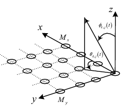
Consider a URA with $M=M_{\mathrm{x}}M_{\mathrm{y}}$ antennas, where $M_{\mathrm{x}}$ and $M_{\mathrm{y}}$ are the numbers of antennas in the x-direction and the y-direction, respectively, as shown in Fig. 1.

Refer to caption — Fig. 1: Array geometry of the URA considered. The direction of the incident path is projected onto the array plane. The angle from the x-axis to the projected line is the azimuth DOA, $\theta_{k,j}(t)$ , and the angle from the z-axis to the incident path is the elevation DOA, $\phi_{k,j}(t)$ . The range of the two parameters are $0\leq\theta_{k,j}(t)<\pi$ and $0\leq\phi_{k,j}(t)<\pi/2$ .

The transmitted signals of all the UTs are in the same frequency band. In the presence of scattering, the received signal at the antenna array is given by [35]

\mathbf{x}(t)=\sum_{k=1}^{K}s_{k}(t)\sum_{j=1}^{N_{k}}\gamma_{k,j}(t)\mathbf{a}(\theta_{k,j}(t),\phi_{k,j}(t))+\mathbf{n}(t)\in\mathbb{C}^{M\times 1},

(1)

where $K$ is the number of the UTs, $s_{k}(t)$ is the complex-valued signal transmitted by the $k$ th UT, and $N_{k}$ is the number of multipaths of the $k$ th UT; $t=1,2,\cdots,T$ is the sampling time, where $T$ is the number of received signal snapshots; $\gamma_{k,j}(t)$ , $\theta_{k,j}(t)$ , and $\phi_{k,j}(t)$ are the complex-valued path gain, the real-valued azimuth DOA, and the real-valued elevation DOA of the $j$ th path from the $k$ th UT, respectively, which satisfy $0\leq\theta_{k,j}(t)<\pi$ and $0\leq\phi_{k,j}(t)<\pi/2$ as shown in Fig. 1; and $\mathbf{n}(t)\in\mathbb{C}^{M\times 1}$ is the complex-valued additive noise. It should be noted that the ranges of the DOAs are the localization ranges of the array, which means that sources out of these ranges cannot be localized by the array. The array manifold, $\mathbf{a}(\theta_{k,j}(t),\phi_{k,j}(t))\in\mathbb{C}^{M\times 1}$ , is the response of the array corresponding to the azimuth and elevation DOAs of $\theta_{k,j}(t)$ and $\phi_{k,j}(t)$ . With respect to the antenna at the origin of the axes, the $m$ th element of $\mathbf{a}(\theta_{k,j}(t),\phi_{k,j}(t))$ is defined as [47]

	$\displaystyle\mspace{-80mu}[\mathbf{a}(\theta_{k,j}(t),\phi_{k,j}(t))]_{m}=\mathrm{exp}\Big(iu\sin(\phi_{k,j}(t))\big[(m_{\mathrm{x}}-1)$
	$\displaystyle\ \ \ \ \ \times\cos(\theta_{k,j}(t))+(m_{\mathrm{y}}-1)\sin(\theta_{k,j}(t))\big]\Big),$
	$\displaystyle m=(m_{\mathrm{y}}-1)M_{\mathrm{x}}+m_{\mathrm{x}},\ m_{\mathrm{x}}=1,2,\cdots,M_{\mathrm{x}},$
	$\displaystyle m_{\mathrm{y}}=1,2,\cdots,M_{\mathrm{y}},$		(2)

where $u=2\pi d/\lambda$ , $d$ is the distance between two adjacent antennas, $\lambda$ is the wavelength. We can see that $[\mathbf{a}(\theta_{k,j}(t),\phi_{k,j}(t))]_{m}$ corresponds to the response of the $(m_{\mathrm{x}},m_{\mathrm{y}})$ th antenna element in the coordinate system shown in Fig. 1. The azimuth and elevation DOAs can be expressed as [35]

	$\displaystyle\theta_{k,j}(t)$	$\displaystyle=$	$\displaystyle\bar{\theta}_{k}+\tilde{\theta}_{k,j}(t),$		(3)
	$\displaystyle\phi_{k,j}(t)$	$\displaystyle=$	$\displaystyle\bar{\phi}_{k}+\tilde{\phi}_{k,j}(t),$		(4)

where $\bar{\theta}_{k}$ and $\bar{\phi}_{k}$ are the real-valued nominal azimuth DOA and the real-valued nominal elevation DOA for the $k$ th UT, and they are the means of $\theta_{k,j}(t)$ and $\phi_{k,j}(t)$ , respectively; $\tilde{\theta}_{k,j}(t)$ and $\tilde{\phi}_{k,j}(t)$ are the corresponding real-valued random angular deviations with zero mean and standard deviations $\sigma_{\theta_{k}}$ and $\sigma_{\phi_{k}}$ , which are referred to as the angular spreads. We emphasize that the task of localization is to estimate the 2-D nominal DOAs, $\bar{\theta}_{k},\ \bar{\phi}_{k},$ and the 2-D angular spreads, $\sigma_{\theta_{k}},\ \sigma_{\phi_{k}},\ k=1,2,\cdots,K$ , with the aid of the received signal snapshots, $\mathbf{x}(t),\ t=1,2,\cdots,T$ . Because the signals of the $K$ UTs are transmitted at the same frequency band and the same time, the received snapshot signals from one UT cannot be extracted from $\mathbf{x}(t),\ t=1,2,\cdots,T$ , regardless of whether the transmitted signals are pilots or data symbols¹¹ 1 When the UTs transmit orthogonal pilots, the BS can correlate the received signals with the known pilots of one UT to extract the signal of that UT. Then, the BS only obtains a rank-1 covariance matrix which is not capable of performing the 2-D localization of the UT.. As a result, the 2-D angular parameters of the $K$ UTs can only be estimated jointly.

In this paper, the following initial assumptions are considered.
1) The angular deviations, $\tilde{\theta}_{k,j}(t)$ and $\tilde{\phi}_{k,j}(t)$ , $k=1,2,\cdots,K$ , $j=1,2,\cdots,N_{k}$ , $t=1,2,\cdots,T$ , are temporally independent and identically distributed (i.i.d.) Gaussian random variables with covariances

\displaystyle{\mathbb{E}}\left\{\tilde{\theta}_{k,j}(t)\tilde{\theta}_{\tilde{k},\tilde{j}}(\tilde{t})\right\}

\displaystyle=

\displaystyle\sigma_{\theta_{k}}^{2}\delta(k-\tilde{k})\delta(j-\tilde{j})\delta(t-\tilde{t}),

(5)

and

\displaystyle{\mathbb{E}}\left\{\tilde{\phi}_{k,j}(t)\tilde{\phi}_{\tilde{k},\tilde{j}}(\tilde{t})\right\}

\displaystyle=

\displaystyle\sigma_{\phi_{k}}^{2}\delta(k-\tilde{k})\delta(j-\tilde{j})\delta(t-\tilde{t}),

(6)

respectively, where the angular spreads, $\sigma_{\theta_{k}}$ and $\sigma_{\phi_{k}}$ , are far less than one.
2) The path gains, $\gamma_{k,j}(t)$ , $k=1,2,\cdots,K$ , $j=1,2,\cdots,N_{k}$ , $t=1,2,\cdots,T$ , are temporally i.i.d. complex-valued zero-mean random variables, whose covariance is

{\mathbb{E}}\left\{{\gamma}_{k,j}(t){\gamma}_{\tilde{k},\tilde{j}}^{*}(\tilde{t})\right\}=\frac{\sigma_{\gamma_{k}}^{2}}{N_{k}}\delta(k-\tilde{k})\delta(j-\tilde{j})\delta(t-\tilde{t}).

(7)

Note that if the path gain factors of different paths are uncorrelated, the sources are said to be ID [18].
3) The noise, $\mathbf{n}(t)$ , $t=1,2,\cdots,T$ are composed of temporally and spatially i.i.d. complex-valued circularly symmetric zero-mean Gaussian variables, whose covariance matrix is given by

{\mathbb{E}}\left\{\mathbf{n}(t)\mathbf{n}^{H}(\tilde{t})\right\}=\sigma_{\mathrm{n}}^{2}\mathbf{I}_{M}\delta(t-\tilde{t}).

(8)

4) The transmitted signals, $s_{k}(t),k=1,2,\cdots,K$ , $t=1,2,\cdots,T$ , are modeled as deterministic ones with constant absolute values, and we denote

S_{k}=\left|s_{k}(t)\right|^{2}

(9)

as the transmitted signal power of the $k$ th UT.
5) The angular deviations, the path gains, the noise, and the transmitted signals are uncorrelated from each other.
6) The array is calibrated, which means the response of the array is known. Hence, the array manifold for any 2-D DOAs, cf. (2), is known a priori. The number of the BS antennas $M$ is much larger than the number of the UTs $K$ .
7) The number of multipaths $N_{k},\forall k$ , is large.

With these assumptions and using the central limit theorem, it can be verified that the received signal vector $\mathbf{x}(t)$ in (1) is a zero-mean circularly symmetric complex-valued Gaussian vector [22], [25], [30], [48].

III The ESPRIT-Based Approach

The existing subspace based and covariance matching approaches are complicated for the 2-D localization in the massive MIMO systems due to the exhausted multidimensional search for estimating the angular parameters. Although the traditional 1-D ESPRIT-based approach avoids searching over the parameter space [19], the angular parameters are mutually coupled when this approach is employed in the 2-D localization straightforwardly. The existing 2-D ESPRIT-based approach decouples the angular parameters, but the azimuth nominal DOA is still estimated with searching, and the angular spreads are not estimated [41]. Hence, in this section, the expression of the signal subspace is first derived, which is the foundation of the ESPRIT-based approaches. Then, the signal subspace based ESPRIT approach is proposed for estimating the 2-D angular parameters without searching.

III-A The Signal Subspace

It can be seen that the array manifold $\mathbf{a}(\theta_{k,j}(t),\phi_{k,j}(t))$ in (2) is a function of the azimuth and elevation DOAs. With the first order Taylor series expansion of $\mathbf{a}(\theta_{k,j}(t),\phi_{k,j}(t))$ around the nominal DOAs, $\bar{\theta}_{k},\bar{\phi}_{k}$ , it can be approximated as

$\displaystyle\mathbf{a}(\theta_{k,j}(t),\phi_{k,j}(t))$	$\displaystyle=$	$\displaystyle\mathbf{a}(\bar{\theta}_{k}+\tilde{\theta}_{k,j}(t),\bar{\phi}_{k}+\tilde{\phi}_{k,j}(t))$	(10)
	$\displaystyle\approx$	$\displaystyle\mathbf{a}(\bar{\theta}_{k},\bar{\phi}_{k})+\frac{\partial\mathbf{a}(\bar{\theta}_{k},\bar{\phi}_{k})}{\partial\bar{\theta}_{k}}\tilde{\theta}_{k,j}(t)$
		$\displaystyle+\frac{\partial\mathbf{a}(\bar{\theta}_{k},\bar{\phi}_{k})}{\partial\bar{\phi}_{k}}\tilde{\phi}_{k,j}(t),$

where the remainder of the series is omitted. It is assumed that the standard deviations of $\tilde{\theta}_{k,j}(t)$ and $\tilde{\phi}_{k,j}(t)$ , i.e., $\sigma_{\theta_{k}}$ and $\sigma_{\phi_{k}}$ , are sufficiently small. Thus, the approximation is almost true. Then, the received signal given by (1) can be rewritten as

	$\displaystyle\mathbf{x}(t)$	$\displaystyle\approx$	$\displaystyle\sum_{k=1}^{K}\Bigg(\mathbf{a}(\bar{\theta}_{k},\bar{\phi}_{k})c_{k,1}(t)+\frac{\partial\mathbf{a}(\bar{\theta}_{k},\bar{\phi}_{k})}{\partial\bar{\theta}_{k}}c_{k,2}(t)$		(11)
			$\displaystyle+\frac{\partial\mathbf{a}(\bar{\theta}_{k},\bar{\phi}_{k})}{\partial\bar{\phi}_{k}}c_{k,3}(t)\Bigg)+\mathbf{n}(t)\in\mathbb{C}^{M\times 1},$		(11)

where

	$\displaystyle c_{k,1}(t)$	$\displaystyle=$	$\displaystyle s_{k}(t)\sum_{j=1}^{N_{k}}\gamma_{k,j}(t),$
	$\displaystyle c_{k,2}(t)$	$\displaystyle=$	$\displaystyle s_{k}(t)\sum_{j=1}^{N_{k}}\gamma_{k,j}(t)\tilde{\theta}_{k,j}(t),$

and

\displaystyle c_{k,3}(t)

\displaystyle=

\displaystyle s_{k}(t)\sum_{j=1}^{N_{k}}\gamma_{k,j}(t)\tilde{\phi}_{k,j}(t).

As a result, if $\mathbf{n}(t)$ is not taken into account, the received signal is linearly related to the array manifold $\mathbf{a}(\bar{\theta}_{k},\bar{\phi}_{k})$ and its partial derivatives. Therefore, it can be concisely expressed as

\mathbf{x}(t)\approx\mathbf{A}\mathbf{c}(t)+\mathbf{n}(t),

(12)

where

	$\displaystyle\mspace{-40mu}\mathbf{A}=\Bigg[\mathbf{a}(\bar{\theta}_{1},\bar{\phi}_{1}),\mathbf{a}(\bar{\theta}_{2},\bar{\phi}_{2}),\cdots,\mathbf{a}(\bar{\theta}_{K},\bar{\phi}_{K}),$
	$\displaystyle\mspace{-40mu}\frac{\partial\mathbf{a}(\bar{\theta}_{1},\bar{\phi}_{1})}{\partial\bar{\theta}_{1}},\frac{\partial\mathbf{a}(\bar{\theta}_{2},\bar{\phi}_{2})}{\partial\bar{\theta}_{2}},\cdots,\frac{\partial\mathbf{a}(\bar{\theta}_{K},\bar{\phi}_{K})}{\partial\bar{\theta}_{K}},$
	$\displaystyle\mspace{-40mu}\frac{\partial\mathbf{a}(\bar{\theta}_{1},\bar{\phi}_{1})}{\partial\bar{\phi}_{1}},\frac{\partial\mathbf{a}(\bar{\theta}_{2},\bar{\phi}_{2})}{\partial\bar{\phi}_{2}},\cdots,\frac{\partial\mathbf{a}(\bar{\theta}_{K},\bar{\phi}_{K})}{\partial\bar{\phi}_{K}}\Bigg]\in\mathbb{C}^{{M}\times 3K}$		(13)

denotes the array response matrix of the URA, and

	$\displaystyle\mspace{-40mu}\mathbf{c}(t)=[c_{1,1}(t),c_{2,1}(t),\cdots,c_{K,1}(t),c_{1,2}(t),c_{2,2}(t),\cdots,$
	$\displaystyle c_{K,2}(t),c_{1,3}(t),c_{2,3}(t),\cdots,c_{K,3}(t)]^{T}\in\mathbb{C}^{3K\times 1}.$

It should be noted that $\mathbf{a}(\bar{\theta}_{k},\bar{\phi}_{k})$ is obtained by changing the DOAs, $\theta_{k,j}(t),\phi_{k,j}(t)$ , in (2) to the nominal DOAs, $\bar{\theta}_{k},\bar{\phi}_{k}$ . We can see that $\mathbf{A}$ is only determined by the nominal DOAs, $\bar{\theta}_{k},\bar{\phi}_{k},k=1,2,\cdots,K$ . Thus, these nominal DOAs might be obtained from $\mathbf{A}$ .

Based on the properties of $\tilde{\theta}_{k,j}(t)$ , $\tilde{\phi}_{k,j}(t)$ , $\gamma_{k,j}(t)$ , and $s_{k}(t)$ that are given in (5), (6), (7), and (9), respectively, and the assumption that the transmitted signals, the path gains, and the angular deviations are uncorrelated from each other, the variances of $c_{k,1}(t)$ , $c_{k,2}(t)$ , and $c_{k,3}(t)$ are obtained as

	$\displaystyle{\mathbb{E}}\left\{c_{k,1}(t)c_{k,1}^{*}(t)\right\}$	$\displaystyle=$	$\displaystyle S_{k}\sigma_{\gamma_{k}}^{2},$		(14)
	$\displaystyle{\mathbb{E}}\left\{c_{k,2}(t)c_{k,2}^{*}(t)\right\}$	$\displaystyle=$	$\displaystyle S_{k}\sigma_{\gamma_{k}}^{2}\sigma_{\theta_{k}}^{2},$		(15)

and

\displaystyle{\mathbb{E}}\left\{c_{k,3}(t)c_{k,3}^{*}(t)\right\}

\displaystyle=

\displaystyle S_{k}\sigma_{\gamma_{k}}^{2}\sigma_{\phi_{k}}^{2},

(16)

respectively. Additionally, the covariance is

{\mathbb{E}}\left\{c_{k,l}(t)c_{\tilde{k},\tilde{l}}^{*}(t)\right\}=0,\forall k\neq\tilde{k},\mathrm{or}\ l\neq\tilde{l}.

(17)

Therefore, the covariance matrix of $\mathbf{c}(t)$ is

\mathbf{\Lambda}_{\mathrm{c}}={\mathbb{E}}\left\{\mathbf{c}(t)\mathbf{c}^{H}(t)\right\}\in\mathbb{R}^{3K\times 3K},

(18)

which is a diagonal matrix with $[\mathbf{\Lambda}_{\mathrm{c}}]_{k,k}=S_{k}\sigma_{\gamma_{k}}^{2}$ , $[\mathbf{\Lambda}_{\mathrm{c}}]_{K+k,K+k}=[\mathbf{\Lambda}_{\mathrm{c}}]_{k,k}\sigma_{\theta_{k}}^{2}$ , $[\mathbf{\Lambda}_{\mathrm{c}}]_{2K+k,2K+k}=[\mathbf{\Lambda}_{\mathrm{c}}]_{k,k}\sigma_{\phi_{k}}^{2}$ , $k=1,2,\cdots,K$ . Therefore, the angular spreads, $\sigma_{\theta_{k}},\sigma_{\phi_{k}},k=1,2,\cdots,K$ , can be obtained from $\mathbf{\Lambda}_{\mathrm{c}}$ .

From (12), we can see that $\mathbf{A}$ and $\mathbf{\Lambda}_{\mathrm{c}}$ might be obtained from the covariance matrix of $\mathbf{x}(t)$ . Since the signal and the noise are uncorrelated from each other, and satisfy (8) and (18), the covariance matrix of the received signal $\mathbf{x}(t)$ given by (12) is thus expressed as

\mathbf{R}_{\mathbf{x}}={\mathbb{E}}\left\{\mathbf{x}(t)\mathbf{x}^{H}(t)\right\}\approx{\mathbf{A}}\mathbf{\Lambda}_{\mathrm{c}}{\mathbf{A}}^{H}+\sigma_{\mathrm{n}}^{2}\mathbf{I}_{M}\in\mathbb{C}^{{M}\times{M}}.

(19)

It can be seen that $\mathbf{R}_{\mathbf{x}}$ is a normal matrix, i.e., $\mathbf{R}_{\mathbf{x}}\mathbf{R}_{\mathbf{x}}^{H}=\mathbf{R}_{\mathbf{x}}^{H}\mathbf{R}_{\mathbf{x}}$ . Because ${\mathbf{A}}\mathbf{\Lambda}_{\mathrm{c}}{\mathbf{A}}^{H}$ is positive semi-definite and $\sigma_{\mathrm{n}}^{2}>0$ , $\mathbf{R}_{\mathbf{x}}$ is positive definite. Thus, the eigenvalue-decomposition (EVD) of $\mathbf{R}_{\mathbf{x}}$ is also the singular value decomposition of $\mathbf{R}_{\mathbf{x}}$ . Let ${\mathbf{A}}$ be a full rank matrix. Then, the largest $3K$ eigenvalues of $\mathbf{R}_{\mathbf{x}}$ are larger than $\sigma_{\mathrm{n}}^{2}$ , and the other $M-3K$ eigenvalues of $\mathbf{R}_{\mathbf{x}}$ approximately equal $\sigma_{\mathrm{n}}^{2}$ . In the next section, we will prove that for the massive MIMO systems ${\mathbf{A}}$ is indeed a full rank matrix. Hence, the EVD of $\mathbf{R}_{\mathbf{x}}$ can be written as

	$\displaystyle\mathbf{R}_{\mathbf{x}}$	$\displaystyle\mspace{-10mu}\approx\mspace{-10mu}$	$\displaystyle[{\mathbf{E}}_{\mathrm{s}},{\mathbf{E}}_{\mathrm{n}}]\left[\begin{array}[]{ll}{\mathbf{\Sigma}}_{\mathrm{s}}&\mathbf{0}_{3K\times(M-3K)}\\ \mathbf{0}_{(M-3K)\times 3K}&\sigma_{\mathrm{n}}^{2}\mathbf{I}_{M-3K}\end{array}\right][{\mathbf{E}}_{\mathrm{s}},{\mathbf{E}}_{\mathrm{n}}]^{H}$		(23)
		$\displaystyle\mspace{-10mu}=\mspace{-10mu}$	$\displaystyle{\mathbf{E}}_{\mathrm{s}}{\mathbf{\Sigma}}_{\mathrm{s}}{\mathbf{E}}_{\mathrm{s}}^{H}+\sigma_{\mathrm{n}}^{2}{\mathbf{E}}_{\mathrm{n}}{\mathbf{E}}_{\mathrm{n}}^{H},$		(23)

where ${\mathbf{E}}_{\mathrm{s}}\in\mathbb{C}^{{M}\times 3K}$ and ${\mathbf{E}}_{\mathrm{n}}\in\mathbb{C}^{{M}\times(M-3K)}$ are composed of the eigenvectors of $\mathbf{R}_{\mathbf{x}}$ , and ${\mathbf{\Sigma}}_{\mathrm{s}}\in\mathbb{R}^{{3K}\times 3K}$ is a diagonal matrix comprising the largest $3K$ eigenvalues of $\mathbf{R}_{\mathbf{x}}$ . It can be seen that $[{\mathbf{E}}_{\mathrm{s}},{\mathbf{E}}_{\mathrm{n}}]\in\mathbb{C}^{{M}\times{M}}$ is a unitary matrix, which satisfies

\mathbf{I}_{M}=[{\mathbf{E}}_{\mathrm{s}},{\mathbf{E}}_{\mathrm{n}}][{\mathbf{E}}_{\mathrm{s}},{\mathbf{E}}_{\mathrm{n}}]^{H}={\mathbf{E}}_{\mathrm{s}}{\mathbf{E}}_{\mathrm{s}}^{H}+{\mathbf{E}}_{\mathrm{n}}{\mathbf{E}}_{\mathrm{n}}^{H},

which means that

{\mathbf{E}}_{\mathrm{n}}{\mathbf{E}}_{\mathrm{n}}^{H}=\mathbf{I}_{M}-{\mathbf{E}}_{\mathrm{s}}{\mathbf{E}}_{\mathrm{s}}^{H}.

(24)

Hence, substituting (24) into (23) yields

\mathbf{R}_{\mathbf{x}}\approx{\mathbf{E}}_{\mathrm{s}}\tilde{\mathbf{\Sigma}}_{\mathrm{s}}{\mathbf{E}}_{\mathrm{s}}^{H}+\sigma_{\mathrm{n}}^{2}\mathbf{I}_{M},

(25)

where $\tilde{\mathbf{\Sigma}}_{\mathrm{s}}={\mathbf{\Sigma}}_{\mathrm{s}}-\sigma_{\mathrm{n}}^{2}\mathbf{I}_{3K}\in\mathbb{R}^{{3K}\times 3K}$ . Then, from (19) and (25), we obtain

{\mathbf{A}}\mathbf{\Lambda}_{\mathrm{c}}{\mathbf{A}}^{H}\approx{\mathbf{E}}_{\mathrm{s}}\tilde{\mathbf{\Sigma}}_{\mathrm{s}}{\mathbf{E}}_{\mathrm{s}}^{H}.

(26)

It is known that the diagonal elements of ${\mathbf{\Sigma}}_{\mathrm{s}}$ are larger than $\sigma_{\mathrm{n}}^{2}$ , which means $\tilde{\mathbf{\Sigma}}_{\mathrm{s}}$ has full rank. Hence, according to the definition of subspace, ${\mathbf{E}}_{\mathrm{s}}$ and ${\mathbf{A}}$ are approximately in the same subspace, i.e.,

{\mathbf{A}}\approx{\mathbf{E}}_{\mathrm{s}}{\mathbf{T}},

(27)

where ${\mathbf{T}}\in\mathbb{C}^{3K\times 3K}$ is a full rank matrix. Additionally, ${\mathbf{E}}_{\mathrm{s}}$ and ${\mathbf{E}}_{\mathrm{n}}$ are termed as the signal subspace and the noise subspace, respectively. It is obvious that the signal subspace can be obtained from the received signal snapshots $\mathbf{x}(t),\ t=1,2,\cdots,T$ , and ${\mathbf{A}}$ is linearly related to the signal subspace. Hence, the linear relation in (27) will be used for estimating the nominal DOAs, and the estimation approach will be given in the next subsection.

III-B The Proposed Estimator

Similar to the practice in the general ESPRIT methods, the antenna array is divided into several subarrays in the proposed estimator as well. Then, the linear relations between the array response matrices of the subarrays can be tactfully constructed for estimating angular parameters. For the estimation of both the elevation and azimuth nominal DOAs, which are coupled in the array manifold, the array has to be divided into at least three subarrays to decouple the 2-D nominal DOAs. This is because obtaining the 2-D nominal DOAs needs at least two different functions of them, which can only be derived from at least two different linear relations between the subarrays, and at least three subarrays are needed to obtain the two linear relations. Although the URA can be divided into more than three subarrays, the computational complexity of estimation increases when the number of the subarrays increases, which constitutes one of the main challenges in the context of the massive MIMO systems. In addition, only one antenna is not used with the three-subarray division, which is rather small in comparison with the total number of antennas $M$ . Therefore, the URA is divided into three subarrays, as shown in Fig. 2. Thus, the proposed approach uses almost all of the BS antennas with low computational complexity.

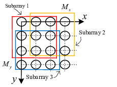
In order to obtain the linear relations between the array response matrices of the subarrays, these array response matrices need to be derived. From (13), it can be seen that the array response matrix $\mathbf{A}$ is constructed by the array manifold $\mathbf{a}(\bar{\theta}_{k},\bar{\phi}_{k})$ and its partial derivatives. Similarly, the array response matrix of each subarray is also constructed by the array manifold of the subarray and its partial derivatives. Hence, the array manifold of each subarray and its partial derivatives will be derived first. The array manifold of the $l$ th subarray corresponding to the nominal DOAs $\bar{\theta}_{k}$ , $\bar{\phi}_{k}$ , cf. (13), is denoted as $\mathbf{a}_{l}(\bar{\theta}_{k},\bar{\phi}_{k})\in\mathbb{C}^{\tilde{M}\times 1}$ , $l=1,2,3$ , where $\tilde{M}=(M_{\mathrm{x}}-1)(M_{\mathrm{y}}-1)$ . Note that $\mathbf{a}_{l}(\bar{\theta}_{k},\bar{\phi}_{k})$ is obtained by selecting the elements of $\mathbf{a}(\bar{\theta}_{k},\bar{\phi}_{k})$ that correspond to the $l$ th subarray and keeping these selected elements in the same order as in $\mathbf{a}(\bar{\theta}_{k},\bar{\phi}_{k})$ . In other words, $\mathbf{a}_{l}(\bar{\theta}_{k},\bar{\phi}_{k})$ can be written as

\mathbf{a}_{l}(\bar{\theta}_{k},\bar{\phi}_{k})=\mathbf{J}_{l}\mathbf{a}(\bar{\theta}_{k},\bar{\phi}_{k}),

(28)

where $\mathbf{J}_{l}\in\mathbb{R}^{\tilde{M}\times M}$ is the selection matrix that assigns the elements of $\mathbf{a}(\bar{\theta}_{k},\bar{\phi}_{k})$ to the $l$ th subarray, and is defined as

[\mathbf{J}_{l}]_{\tilde{m},\tilde{n}}=\left\{\begin{array}[]{ll}1,&\tilde{n}=\tilde{m}+\lfloor\frac{\tilde{m}-1}{M_{\mathrm{x}}-1}\rfloor+d_{l},\tilde{m}=1,2,\cdots,\tilde{M},\\ 0,&\mathrm{otherwise},\end{array}\right.

in which $d_{1}=0,\ d_{2}=1$ , and $d_{3}=M_{\mathrm{x}}$ . In the above equation, the floor operator makes $\lfloor\frac{\tilde{m}-1}{M_{\mathrm{x}}-1}\rfloor=n,\forall n=0,1,\cdots,M_{\mathrm{y}}-2$ when $\tilde{m}=n(M_{\mathrm{x}}-1)+1,n(M_{\mathrm{x}}-1)+2,\cdots,(n+1)(M_{\mathrm{x}}-1)$ . It can be seen that for the $\tilde{m}$ th row of $\mathbf{J}_{l}$ , only the ( $\tilde{m}+\lfloor\frac{\tilde{m}-1}{M_{\mathrm{x}}-1}\rfloor+d_{l}$ )th entry is one, and the other entries are zeros. Thus, $\mathbf{J}_{l}$ assigns the ( $\tilde{m}+\lfloor\frac{\tilde{m}-1}{M_{\mathrm{x}}-1}\rfloor+d_{l}$ )th entry of $\mathbf{a}(\bar{\theta}_{k},\bar{\phi}_{k})$ to the $\tilde{m}$ th entry of $\mathbf{a}_{l}(\bar{\theta}_{k},\bar{\phi}_{k})$ , and this coincides with the relation between the subarrays and the URA. From the definition of $\mathbf{a}_{l}(\bar{\theta}_{k},\bar{\phi}_{k})$ , it can be found that the array manifolds of different subarrays are linearly related as

\displaystyle\mathbf{a}_{q}(\bar{\theta}_{k},\bar{\phi}_{k})=F_{q}(\bar{\theta}_{k},\bar{\phi}_{k})\mathbf{a}_{1}(\bar{\theta}_{k},\bar{\phi}_{k}),

(29)

where $q=2,3$ , and

	$\displaystyle F_{2}(\bar{\theta}_{k},\bar{\phi}_{k})$	$\displaystyle=$	$\displaystyle\mathrm{exp}(iu\sin(\bar{\phi}_{k})\cos(\bar{\theta}_{k})),$		(30)
	$\displaystyle F_{3}(\bar{\theta}_{k},\bar{\phi}_{k})$	$\displaystyle=$	$\displaystyle\mathrm{exp}(iu\sin(\bar{\phi}_{k})\sin(\bar{\theta}_{k})).$		(31)

Note that $F_{2}(\bar{\theta}_{k},\bar{\phi}_{k})$ and $F_{3}(\bar{\theta}_{k},\bar{\phi}_{k})$ are two different functions of the 2-D nominal DOAs, $\bar{\theta}_{k}$ , $\bar{\phi}_{k}$ , and can be exploited to estimate these nominal DOAs. After computing the partial derivatives of $\mathbf{a}_{q}(\bar{\theta}_{k},\bar{\phi}_{k})$ , we can see that they are related to $\mathbf{a}_{1}(\bar{\theta}_{k},\bar{\phi}_{k})$ and its partial derivatives as

	$\displaystyle\mspace{-30mu}\frac{\partial\mathbf{a}_{q}(\bar{\theta}_{k},\bar{\phi}_{k})}{\partial\theta}=F_{q}(\bar{\theta}_{k},\bar{\phi}_{k})\frac{\partial\mathbf{a}_{1}(\bar{\theta}_{k},\bar{\phi}_{k})}{\partial\theta}$
	$\displaystyle\mspace{80mu}+\frac{\partial F_{q}(\bar{\theta}_{k},\bar{\phi}_{k})}{\partial\theta}\mathbf{a}_{1}(\bar{\theta}_{k},\bar{\phi}_{k}),$		(32)

and

	$\displaystyle\mspace{-30mu}\frac{\partial\mathbf{a}_{q}(\bar{\theta}_{k},\bar{\phi}_{k})}{\partial\phi}=F_{q}(\bar{\theta}_{k},\bar{\phi}_{k})\frac{\partial\mathbf{a}_{1}(\bar{\theta}_{k},\bar{\phi}_{k})}{\partial\phi}$
	$\displaystyle\mspace{80mu}+\frac{\partial F_{q}(\bar{\theta}_{k},\bar{\phi}_{k})}{\partial\phi}\mathbf{a}_{1}(\bar{\theta}_{k},\bar{\phi}_{k}).$		(33)

In the existing ESPRIT-based approaches [19], [41], the partial derivatives, ${\partial F_{q}(\bar{\theta}_{k},\bar{\phi}_{k})}/{\partial\theta}$ and ${\partial F_{q}(\bar{\theta}_{k},\bar{\phi}_{k})}/{\partial\phi}$ , are approximated as zero, which is based on the assumption that the distance between adjacent antennas $d$ is much shorter than the wavelength $\lambda$ . In fact, $d$ might not satisfy this assumption. These partial derivatives in (32) and (33) do not vanish. Therefore, this restriction on $d$ is not needed in our derivation.

By replacing $\mathbf{a}(\bar{\theta}_{k},\bar{\phi}_{k})$ , ${\partial\mathbf{a}(\bar{\theta}_{k},\bar{\phi}_{k})}/{\partial\bar{\theta}_{k}}$ , and ${\partial\mathbf{a}(\bar{\theta}_{k},\bar{\phi}_{k})}/{\partial\bar{\phi}_{k}}$ in (13) with $\mathbf{a}_{l}(\bar{\theta}_{k},\bar{\phi}_{k})$ , ${\partial\mathbf{a}_{l}(\bar{\theta}_{k},\bar{\phi}_{k})}/{\partial\bar{\theta}_{k}}$ , and ${\partial\mathbf{a}_{l}(\bar{\theta}_{k},\bar{\phi}_{k})}/{\partial\bar{\phi}_{k}}$ , respectively, the array response matrix of the $l$ th subarray is expressed as

	$\displaystyle\mspace{-50mu}\mathbf{A}_{l}=\Bigg[\mathbf{a}_{l}(\bar{\theta}_{1},\bar{\phi}_{1}),\mathbf{a}_{l}(\bar{\theta}_{2},\bar{\phi}_{2}),\cdots,\mathbf{a}_{l}(\bar{\theta}_{K},\bar{\phi}_{K}),$
	$\displaystyle\mspace{-62mu}\frac{\partial\mathbf{a}_{l}(\bar{\theta}_{1},\bar{\phi}_{1})}{\partial\bar{\theta}_{1}},\frac{\partial\mathbf{a}_{l}(\bar{\theta}_{2},\bar{\phi}_{2})}{\partial\bar{\theta}_{2}},\cdots,\frac{\partial\mathbf{a}_{l}(\bar{\theta}_{K},\bar{\phi}_{K})}{\partial\bar{\theta}_{K}},$
	$\displaystyle\mspace{-62mu}\frac{\partial\mathbf{a}_{l}(\bar{\theta}_{1},\bar{\phi}_{1})}{\partial\bar{\phi}_{1}},\frac{\partial\mathbf{a}_{l}(\bar{\theta}_{2},\bar{\phi}_{2})}{\partial\bar{\phi}_{2}},\cdots,\frac{\partial\mathbf{a}_{l}(\bar{\theta}_{K},\bar{\phi}_{K})}{\partial\bar{\phi}_{K}}\Bigg]\in\mathbb{C}^{\tilde{M}\times 3K}.$		(34)

Then, from (29) and (32)-(34), we can see that the array response matrices of the subarrays are linearly related as

\mathbf{A}_{q}=\mathbf{A}_{1}\mathbf{\Phi}_{q,1},

(35)

where

\mathbf{\Phi}_{q,1}=\left[\begin{array}[]{lll}\mathbf{\Lambda}_{q,1}&\mathbf{\Lambda}_{q,2}&\mathbf{\Lambda}_{q,3}\\ \mathbf{0}_{K\times K}&\mathbf{\Lambda}_{q,1}&\mathbf{0}_{K\times K}\\ \mathbf{0}_{K\times K}&\mathbf{0}_{K\times K}&\mathbf{\Lambda}_{q,1}\end{array}\right]\in\mathbb{C}^{3K\times 3K},

(36)

	$\displaystyle\mspace{-35mu}\mathbf{\Lambda}_{q,1}=\mathrm{diag}\left(F_{q}(\bar{\theta}_{1},\bar{\phi}_{1}),F_{q}(\bar{\theta}_{2},\bar{\phi}_{2}),\cdots,F_{q}(\bar{\theta}_{K},\bar{\phi}_{K})\right)$
	$\displaystyle\ \in\mathbb{C}^{K\times K},$

	$\displaystyle\mspace{-35mu}\mathbf{\Lambda}_{q,2}=\mathrm{diag}\left(\frac{\partial F_{q}(\bar{\theta}_{1},\bar{\phi}_{1})}{\partial\bar{\theta}_{1}},\frac{\partial F_{q}(\bar{\theta}_{2},\bar{\phi}_{2})}{\partial\bar{\theta}_{2}},\cdots,\frac{\partial F_{q}(\bar{\theta}_{K},\bar{\phi}_{K})}{\partial\bar{\theta}_{K}}\right)$
	$\displaystyle\ \in\mathbb{C}^{K\times K},$

and

	$\displaystyle\mspace{-35mu}\mathbf{\Lambda}_{q,3}=\mathrm{diag}\left(\frac{\partial F_{q}(\bar{\theta}_{1},\bar{\phi}_{1})}{\partial\bar{\phi}_{1}},\frac{\partial F_{q}(\bar{\theta}_{2},\bar{\phi}_{2})}{\partial\bar{\phi}_{2}},\cdots,\frac{\partial F_{q}(\bar{\theta}_{K},\bar{\phi}_{K})}{\partial\bar{\phi}_{K}}\right)$
	$\displaystyle\ \in\mathbb{C}^{K\times K}.$

From (30), (31), and (36), we know that the diagonal elements of $\mathbf{\Phi}_{q,1}$ are functions of the 2-D nominal DOAs and can be expressed as

	$\displaystyle[\mathbf{\Phi}_{2,1}]_{k+(l-1)K,k+(l-1)K}$	$\displaystyle\mspace{-10mu}=\mspace{-10mu}$	$\displaystyle\mathrm{exp}(iu\sin(\bar{\phi}_{k})\cos(\bar{\theta}_{k})),$		(37)
	$\displaystyle[\mathbf{\Phi}_{3,1}]_{k+(l-1)K,k+(l-1)K}$	$\displaystyle\mspace{-10mu}=\mspace{-10mu}$	$\displaystyle\mathrm{exp}(iu\sin(\bar{\phi}_{k})\sin(\bar{\theta}_{k})),$		(38)

where $l=1,2,3$ . Hence, the diagonal elements of $\mathbf{\Phi}_{q,1}$ will be used for estimating the nominal DOAs.

On the other hand, the array response matrix $\mathbf{A}_{l}$ of the $l$ th subarray is also linearly related to the signal subspace ${\mathbf{E}}_{\mathrm{s}}$ . By substituting (28) into (34), the array response matrix of the $l$ th subarray is expressed as

$\displaystyle\mathbf{A}_{l}$	$\displaystyle=$	$\displaystyle\mathbf{J}_{l}\mathbf{A}$	(39)
	$\displaystyle\approx$	$\displaystyle\mathbf{J}_{l}{\mathbf{E}}_{\mathrm{s}}{\mathbf{T}}$	(40)
	$\displaystyle=$	$\displaystyle{\mathbf{E}}_{l}{\mathbf{T}},\ \ \ l=1,2,3,$	(41)

where (40) is derived by substituting (27) into (39), and

{\mathbf{E}}_{l}\triangleq\mathbf{J}_{l}{\mathbf{E}}_{\mathrm{s}}\in\mathbb{C}^{\tilde{M}\times 3K},\ \ \ l=1,2,3,

(42)

are termed as the selected signal subspaces. It can be seen that the array response matrix $\mathbf{A}_{l}$ of the $l$ th subarray, cf. (39), and the selected signal subspace ${\mathbf{E}}_{l}$ of the $l$ th subarray, cf. (42), are selected in the same way. Because the signal subspace ${\mathbf{E}}_{\mathrm{s}}$ and the array response matrix $\mathbf{A}$ are linearly related, cf. (27), we discover that the selected signal subspace ${\mathbf{E}}_{l}$ and the array response matrix $\mathbf{A}_{l}$ of the $l$ th subarray are linearly related. Therefore, it is proved that ${\mathbf{E}}_{l},l=1,2,3$ , are linearly related with each other in a similar way to $\mathbf{A}_{l}$ in (35), which is exploited to obtain the diagonal elements of $\mathbf{\Phi}_{2,1}$ and $\mathbf{\Phi}_{3,1}$ . These diagonal elements are different functions of the 2-D nominal DOAs, cf. (36).

Because only the selected signal subspace ${\mathbf{E}}_{l}$ can be obtained from the received signal snapshots, $\mathbf{A}_{l}$ in (35) needs to be written as the linear transformation of ${\mathbf{E}}_{l}$ for obtaining the diagonal elements of $\mathbf{\Phi}_{2,1}$ and $\mathbf{\Phi}_{3,1}$ . Combining (35) and (41), we get

	$\displaystyle\mathbf{A}_{1}$	$\displaystyle\approx$	$\displaystyle{\mathbf{E}}_{1}{\mathbf{T}},$		(43)
	$\displaystyle\mathbf{A}_{1}\mathbf{\Phi}_{2,1}$	$\displaystyle\approx$	$\displaystyle{\mathbf{E}}_{2}{\mathbf{T}},$		(44)

and

\mathbf{A}_{1}\mathbf{\Phi}_{3,1}\approx{\mathbf{E}}_{3}{\mathbf{T}}.

(45)

Note that $\mathbf{A}_{1}$ is linearly related to all the selected signal subspaces. Substituting (43) into (44) and (45) yields

{\mathbf{E}}_{1}\mathbf{\Psi}_{1}\approx{\mathbf{E}}_{2},

(46)

and

{\mathbf{E}}_{1}\mathbf{\Psi}_{2}\approx{\mathbf{E}}_{3},

(47)

where

\mathbf{\Psi}_{1}={\mathbf{T}}\mathbf{\Phi}_{2,1}{\mathbf{T}}^{-1}\in\mathbb{C}^{3K\times 3K},

(48)

and

\mathbf{\Psi}_{2}={\mathbf{T}}\mathbf{\Phi}_{3,1}{\mathbf{T}}^{-1}\in\mathbb{C}^{3K\times 3K}.

(49)

Obviously, the diagonal elements of $\mathbf{\Phi}_{2,1}$ and $\mathbf{\Phi}_{3,1}$ are the eigenvalues of $\mathbf{\Psi}_{1}$ and $\mathbf{\Psi}_{2}$ , respectively, which is because $\mathbf{\Phi}_{2,1}$ and $\mathbf{\Phi}_{3,1}$ are upper triangular matrices. Therefore, in order to estimate the diagonal elements of $\mathbf{\Phi}_{2,1}$ and $\mathbf{\Phi}_{3,1}$ , $\mathbf{\Psi}_{1}$ and $\mathbf{\Psi}_{2}$ need to be estimated from the selected signal subspaces ${\mathbf{E}}_{l},l=1,2,3$ . According to (46) and (47), they can be obtained by employing the well-known total least-squares (TLS) criterion [45]. First, compute the EVD as

	$\displaystyle[{\mathbf{E}}_{1},{\mathbf{E}}_{2}]^{H}[{\mathbf{E}}_{1},{\mathbf{E}}_{2}]$	$\displaystyle=$	$\displaystyle{\mathbf{E}}_{\mathrm{x}}\mathbf{\Lambda}_{\mathrm{x}}{\mathbf{E}}_{\mathrm{x}}^{H}\in\mathbb{C}^{6K\times 6K},$		(50)
	$\displaystyle{[{\mathbf{E}}_{1},{\mathbf{E}}_{3}]}^{H}[{\mathbf{E}}_{1},{\mathbf{E}}_{3}]$	$\displaystyle=$	$\displaystyle{\mathbf{E}}_{\mathrm{y}}\mathbf{\Lambda}_{\mathrm{y}}{\mathbf{E}}_{\mathrm{y}}^{H}\in\mathbb{C}^{6K\times 6K},$		(51)

where the columns of ${\mathbf{E}}_{\mathrm{x}}\in\mathbb{C}^{6K\times 6K}$ and ${\mathbf{E}}_{\mathrm{y}}\in\mathbb{C}^{6K\times 6K}$ are the eigenvectors of the left-hand side matrices of (50) and (51), respectively, while the diagonal elements of $\mathbf{\Lambda}_{\mathrm{x}}\in\mathbb{C}^{6K\times 6K}$ and $\mathbf{\Lambda}_{\mathrm{y}}\in\mathbb{C}^{6K\times 6K}$ are their respective eigenvalues, which are placed in descending order from the upper left corner. Then, ${\mathbf{E}}_{\mathrm{x}}$ and ${\mathbf{E}}_{\mathrm{y}}$ are partitioned as

{\mathbf{E}}_{\mathrm{x}}=\left[\begin{array}[]{ll}\mathbf{E}_{{\mathrm{x}}11}&\mathbf{E}_{{\mathrm{x}}12}\\ \mathbf{E}_{{\mathrm{x}}21}&\mathbf{E}_{{\mathrm{x}}22}\end{array}\right],\ \ {\mathbf{E}}_{\mathrm{y}}=\left[\begin{array}[]{ll}\mathbf{E}_{{\mathrm{y}}11}&\mathbf{E}_{{\mathrm{y}}12}\\ \mathbf{E}_{{\mathrm{y}}21}&\mathbf{E}_{{\mathrm{y}}22}\end{array}\right],

(52)

where $\mathbf{E}_{{\mathrm{x}}ab}\in\mathbb{C}^{3K\times 3K},\mathbf{E}_{{\mathrm{y}}ab}\in\mathbb{C}^{3K\times 3K},\ a,b=1,2$ . Finally, $\mathbf{\Psi}_{1}$ and $\mathbf{\Psi}_{2}$ can be estimated as

	$\displaystyle\hat{\mathbf{\Psi}}_{1}$	$\displaystyle=$	$\displaystyle-\mathbf{E}_{{\mathrm{x}}12}\mathbf{E}_{{\mathrm{x}}22}^{-1}\in\mathbb{C}^{3K\times 3K},$		(53)
	$\displaystyle\hat{\mathbf{\Psi}}_{2}$	$\displaystyle=$	$\displaystyle-\mathbf{E}_{{\mathrm{y}}12}\mathbf{E}_{{\mathrm{y}}22}^{-1}\in\mathbb{C}^{3K\times 3K},$		(54)

and we have $\hat{\mathbf{\Psi}}_{1}\approx{\mathbf{\Psi}}_{1}$ , $\hat{\mathbf{\Psi}}_{2}\approx{\mathbf{\Psi}}_{2}$ .

For estimating the nominal DOAs, we calculate the EVD of $\hat{\mathbf{\Psi}}_{1}$ and $\hat{\mathbf{\Psi}}_{2}$ as

	$\displaystyle\hat{\mathbf{\Psi}}_{1}$	$\displaystyle=$	$\displaystyle{\mathbf{T}}_{1}\mathbf{\Lambda}_{1}{\mathbf{T}}_{1}^{-1},$		(55)
	$\displaystyle\hat{\mathbf{\Psi}}_{2}$	$\displaystyle=$	$\displaystyle{\mathbf{T}}_{2}\mathbf{\Lambda}_{2}{\mathbf{T}}_{2}^{-1},$		(56)

where ${\mathbf{T}}_{1}\in\mathbb{C}^{3K\times 3K}$ and ${\mathbf{T}}_{2}\in\mathbb{C}^{3K\times 3K}$ are composed of the eigenvectors of $\hat{\mathbf{\Psi}}_{1}$ and $\hat{\mathbf{\Psi}}_{2}$ , respectively, while $\mathbf{\Lambda}_{1}\in\mathbb{C}^{3K\times 3K}$ and $\mathbf{\Lambda}_{2}\in\mathbb{C}^{3K\times 3K}$ are diagonal matrices whose diagonal elements are the corresponding eigenvalues, which are placed in descending order from the upper left corner. From the previous analysis, the diagonal elements of $\mathbf{\Lambda}_{1}$ and $\mathbf{\Lambda}_{2}$ can be taken as the estimates of the diagonal elements of $\mathbf{\Phi}_{2,1}$ and $\mathbf{\Phi}_{3,1}$ . However, the diagonal elements of $\mathbf{\Lambda}_{1}$ and $\mathbf{\Lambda}_{2}$ are in different order compared with the diagonal elements of $\mathbf{\Phi}_{2,1}$ and $\mathbf{\Phi}_{3,1}$ , which means the diagonal elements of $\mathbf{\Lambda}_{1}$ and $\mathbf{\Lambda}_{2}$ are mismatched. Therefore, these elements should be matched before the nominal DOAs are estimated.

From the definition of $\mathbf{\Phi}_{q,1}$ given in (36), we can see that $\mathbf{\Phi}_{2,1}\mathbf{\Phi}_{3,1}\in\mathbb{C}^{3K\times 3K}$ and $\mathbf{\Phi}_{2,1}\mathbf{\Phi}_{3,1}^{-1}\in\mathbb{C}^{3K\times 3K}$ are also upper triangular matrices, and their diagonal elements satisfy $[\mathbf{\Phi}_{2,1}\mathbf{\Phi}_{3,1}]_{p,p}=[\mathbf{\Phi}_{2,1}]_{p,p}[\mathbf{\Phi}_{3,1}]_{p,p}$ and $[\mathbf{\Phi}_{2,1}\mathbf{\Phi}_{3,1}^{-1}]_{p,p}=[\mathbf{\Phi}_{2,1}]_{p,p}/[\mathbf{\Phi}_{3,1}]_{p,p},\ p=1,2,\cdots,3K$ , respectively. In addition, according to (48) and (49), we have

	$\displaystyle\hat{\mathbf{\Psi}}_{3}=\hat{\mathbf{\Psi}}_{1}\hat{\mathbf{\Psi}}_{2}\approx{\mathbf{T}}\mathbf{\Phi}_{2,1}\mathbf{\Phi}_{3,1}{\mathbf{T}}^{-1}\in\mathbb{C}^{3K\times 3K},$		(57)
	$\displaystyle\hat{\mathbf{\Psi}}_{4}=\hat{\mathbf{\Psi}}_{1}\hat{\mathbf{\Psi}}_{2}^{-1}\approx{\mathbf{T}}\mathbf{\Phi}_{2,1}\mathbf{\Phi}_{3,1}^{-1}{\mathbf{T}}^{-1}\in\mathbb{C}^{3K\times 3K}.$		(58)

Therefore, the eigenvalues of $\hat{\mathbf{\Psi}}_{3}$ are approximately the diagonal elements of $\mathbf{\Phi}_{2,1}\mathbf{\Phi}_{3,1}$ . In addition, denote the EVD of ${\mathbf{\Psi}}_{3}$ as

\hat{\mathbf{\Psi}}_{3}={\mathbf{T}}_{3}\mathbf{\Lambda}_{3}{\mathbf{T}}_{3}^{-1},

(59)

where ${\mathbf{T}}_{3}\in\mathbb{C}^{3K\times 3K}$ is composed of the eigenvectors of $\mathbf{\Psi}_{3}$ , and $\mathbf{\Lambda}_{3}\in\mathbb{C}^{3K\times 3K}$ is a diagonal matrix composed of the eigenvalues of $\mathbf{\Psi}_{3}$ . From (57) and (59), we have

\mathbf{\Lambda}_{3}={\mathbf{T}}_{3}^{-1}\hat{\mathbf{\Psi}}_{3}{\mathbf{T}}_{3}\approx{\mathbf{T}}_{3}^{-1}{\mathbf{T}}\mathbf{\Phi}_{2,1}\mathbf{\Phi}_{3,1}{\mathbf{T}}^{-1}{\mathbf{T}}_{3},

(60)

in which the diagonal elements of $\mathbf{\Phi}_{2,1}\mathbf{\Phi}_{3,1}$ approximately formulate the diagonal elements of $\mathbf{\Lambda}_{3}$ . Similarly, denote

\tilde{\mathbf{\Psi}}_{4}={\mathbf{T}}_{3}^{-1}\hat{\mathbf{\Psi}}_{4}{\mathbf{T}}_{3}\in\mathbb{C}^{3K\times 3K}.

(61)

Substituting (58) into (61) yields

\tilde{\mathbf{\Psi}}_{4}\approx{\mathbf{T}}_{3}^{-1}{\mathbf{T}}\mathbf{\Phi}_{2,1}\mathbf{\Phi}_{3,1}^{-1}{\mathbf{T}}^{-1}{\mathbf{T}}_{3}.

(62)

Comparing (60) and (62), we know that the diagonal elements of $\mathbf{\Phi}_{2,1}\mathbf{\Phi}_{3,1}^{-1}$ approximately formulate the diagonal elements of $\tilde{\mathbf{\Psi}}_{4}$ in the same manner as formulating the diagonal elements of $\mathbf{\Lambda}_{3}$ with the diagonal elements of $\mathbf{\Phi}_{2,1}\mathbf{\Phi}_{3,1}$ . More specifically, if $[\mathbf{\Lambda}_{3}]_{p,p}\approx[\mathbf{\Phi}_{2,1}]_{c_{p},c_{p}}[\mathbf{\Phi}_{3,1}]_{c_{p},c_{p}},\forall p$ , where $c_{p}\in\{1,2,\cdots,3K\}$ and it varies with $p$ . Then, we have $[\tilde{\mathbf{\Psi}}_{4}]_{p,p}\approx[\mathbf{\Phi}_{2,1}]_{c_{p},c_{p}}/[\mathbf{\Phi}_{3,1}]_{c_{p},c_{p}}$ . These facts can be exploited to match the diagonal elements of $\mathbf{\Lambda}_{1}$ and $\mathbf{\Lambda}_{2}$ . A matching algorithm is proposed as follows.

Algorithm 1: Matching of the Eigenvalues

Calculate the EVD of $\hat{\mathbf{\Psi}}_{1}$ and $\hat{\mathbf{\Psi}}_{2}$ using (55) and (56).

Calculate the EVD of $\hat{\mathbf{\Psi}}_{3}$ as (59). Calculate $\tilde{\mathbf{\Psi}}_{4}$ as (61). Set $p=0$ .

$p\leftarrow p+1$ .

•

Calculate the product $\beta_{p,\tilde{p},1}=[\mathbf{\Lambda}_{1}]_{p,p}[\mathbf{\Lambda}_{2}]_{\tilde{p},\tilde{p}}$ and the quotient $\beta_{p,\tilde{p},2}=[\mathbf{\Lambda}_{1}]_{p,p}/[\mathbf{\Lambda}_{2}]_{\tilde{p},\tilde{p}}$ , where $\tilde{p}=1,2,\cdots,3K$ .
•

Match $\beta_{p,\tilde{p},1}$ and $[\mathbf{\Lambda}_{3}]_{p^{\prime},p^{\prime}}$ , $\beta_{p,\tilde{p},2}$ and $[\tilde{\mathbf{\Psi}}_{4}]_{p^{\prime},p^{\prime}}$ , $p^{\prime}=1,2,\cdots,3K$ , according to the LS criterion, i.e., find the corresponding relation between $\mathbf{\Lambda}_{1}$ and $\mathbf{\Lambda}_{2}$ based on $(x_{p},y_{p})=\arg\min_{\tilde{p},p^{\prime}}\mu_{p,\tilde{p},p^{\prime}}$ , where $\mu_{p,\tilde{p},p^{\prime}}=\left|\beta_{p,\tilde{p},1}-[\mathbf{\Lambda}_{3}]_{p^{\prime},p^{\prime}}\right|^{2}+\left|\beta_{p,\tilde{p},2}-[\tilde{\mathbf{\Psi}}_{4}]_{p^{\prime},p^{\prime}}\right|^{2}$ .
•

Set $[\tilde{\mathbf{\Lambda}}_{2}]_{p,p}=[{\mathbf{\Lambda}}_{2}]_{x_{p},x_{p}}$ , where ${\tilde{\mathbf{\Lambda}}_{2}}\in\mathbb{C}^{3K\times 3K}$ is a diagonal matrix.

Repeat Step 3 until $p=3K$ . 5 Sort the diagonal elements of $\mathbf{\Lambda}_{1}$ in descending order, and the $p$ th largest element of $\mathbf{\Lambda}_{1}$ is given by $\lambda_{1,p}=[\mathbf{\Lambda}_{1}]_{z_{p},z_{p}},p=1,2,\cdots,3K$ , where $z_{p}\in\{1,2,\cdots,3K\}$ represents the position of the $p$ th largest element of $\mathbf{\Lambda}_{1}$ and can be obtained by sorting the diagonal elements of $\mathbf{\Lambda}_{1}$ . Additionally, the diagonal elements of $\tilde{\mathbf{\Lambda}}_{2}$ are sorted according to $z_{p},p=1,2,\cdots,3K$ , and the $p$ th sorted element is given by $\lambda_{2,p}=[\tilde{\mathbf{\Lambda}}_{2}]_{z_{p},z_{p}},p=1,2,\cdots,3K$ .

	$\displaystyle\mspace{-20mu}\hat{\bar{\theta}}_{k}$	$\displaystyle\mspace{-10mu}=\mspace{-10mu}$	$\displaystyle\frac{1}{3}\sum_{l=1}^{3}\arctan\left(\frac{\ln\left(\lambda_{2,3(k-1)+l}\right)}{\ln\left(\lambda_{1,3(k-1)+l}\right)}\right),$		(65)
	$\displaystyle\mspace{-20mu}\hat{\bar{\phi}}_{k}$	$\displaystyle\mspace{-10mu}=\mspace{-10mu}$	$\displaystyle\frac{1}{3}\sum_{l=1}^{3}\arcsin\left(\frac{1}{u}\sqrt{-\sum_{a=1}^{2}\left(\ln\left(\lambda_{a,3(k-1)+l}\right)\right)^{2}}\right),$		(66)

	$\displaystyle\hat{\sigma}_{\theta_{k}}$	$\displaystyle=$	$\displaystyle\sqrt{\frac{[\hat{\mathbf{\Lambda}}_{\mathrm{c}}]_{K+k,K+k}}{[\hat{\mathbf{\Lambda}}_{\mathrm{c}}]_{k,k}}},$		(68)
	$\displaystyle\hat{\sigma}_{\phi_{k}}$	$\displaystyle=$	$\displaystyle\sqrt{\frac{[\hat{\mathbf{\Lambda}}_{\mathrm{c}}]_{2K+k,2K+k}}{[\hat{\mathbf{\Lambda}}_{\mathrm{c}}]_{k,k}}},$		(69)

COMET [35]	$O(D_{1}M^{3})$
Subspace estimator [40]	$O(D_{2}M^{3})$
DISPARE [37]	$O(D_{2}M^{3})$
The proposed estimator	$O(M^{3})$

$\displaystyle\left[\frac{\partial\mathbf{a}(\bar{\theta}_{k},\bar{\phi}_{k})}{\partial\bar{\theta}_{k}}\right]_{m}$	$\displaystyle=$	$\displaystyle iu\sin(\bar{\phi}_{k})\Big[-(m_{\mathrm{x}}-1)\sin(\bar{\theta}_{k})$	(80)
		$\displaystyle\mspace{-50mu}+(m_{\mathrm{y}}-1)\cos(\bar{\theta}_{k})\Big]\times[{\mathbf{a}(\bar{\theta}_{k},\bar{\phi}_{k})}]_{m},$	(80)
$\displaystyle{\left[\frac{\partial\mathbf{a}(\bar{\theta}_{k},\bar{\phi}_{k})}{\partial\bar{\phi}_{k}}\right]}_{m}$	$\displaystyle=$	$\displaystyle iu\cos(\bar{\phi}_{k})\big[(m_{\mathrm{x}}-1)\cos(\bar{\theta}_{k})$	(81)
		$\displaystyle\mspace{-50mu}+(m_{\mathrm{y}}-1)\sin(\bar{\theta}_{k})\big]\times[{\mathbf{a}(\bar{\theta}_{k},\bar{\phi}_{k})}]_{m},$	(81)

$\displaystyle r_{k,1}$	$\displaystyle\mspace{-10mu}=\mspace{-10mu}$	$\displaystyle\sqrt{{\mathbf{a}^{H}(\bar{\theta}_{k},\bar{\phi}_{k})}\mathbf{a}(\bar{\theta}_{k},\bar{\phi}_{k})}=\sqrt{M},$	(82)
$\displaystyle r_{k,2}$	$\displaystyle\mspace{-10mu}=\mspace{-10mu}$	$\displaystyle\sqrt{{\left(\frac{\partial\mathbf{a}(\bar{\theta}_{k},\bar{\phi}_{k})}{\partial\bar{\theta}_{k}}\right)}^{H}\frac{\partial\mathbf{a}(\bar{\theta}_{k},\bar{\phi}_{k})}{\partial\bar{\theta}_{k}}}=\sqrt{M\tilde{M}}\tilde{r}_{k,2},$	(83)
$\displaystyle r_{k,3}$	$\displaystyle\mspace{-10mu}=\mspace{-10mu}$	$\displaystyle\sqrt{{\left(\frac{\partial\mathbf{a}(\bar{\theta}_{k},\bar{\phi}_{k})}{\partial\bar{\phi}_{k}}\right)}^{H}\frac{\partial\mathbf{a}(\bar{\theta}_{k},\bar{\phi}_{k})}{\partial\bar{\phi}_{k}}}=\sqrt{M\tilde{M}}\tilde{r}_{k,3},$	(84)

Abstract

Index Terms:

I Introduction

II System Model

III The ESPRIT-Based Approach

III-A The Signal Subspace

III-B The Proposed Estimator

Remark 1

Remark 2

IV Analysis of the Proposed Approach

IV-A The Impact of the Number of the BS Antennas

Proposition 1

Proof:

Remark 3

IV-B Approximate CRB of the Proposed Estimator

Remark 4

IV-C Complexity Analysis

V Numerical Results

VI Conclusions

Acknowledgment

Appendix A Proof of Proposition 1

Appendix B Derivation of the Approximate CRB

References

	$\displaystyle\lambda_{1,3(k-1)+l}$	$\displaystyle\approx$	$\displaystyle\mathrm{exp}(iu\sin(\bar{\phi}_{k})\cos(\bar{\theta}_{k})),$		(63)
	$\displaystyle\lambda_{2,3(k-1)+l}$	$\displaystyle\approx$	$\displaystyle\mathrm{exp}(iu\sin(\bar{\phi}_{k})\sin(\bar{\theta}_{k})),$		(64)

	$\displaystyle\mspace{-30mu}\hat{\mathbf{R}}_{\mathrm{n}}=\frac{1}{T}\sum_{t=1}^{T}\left(\mathbf{A}\mathbf{c}(t)\mathbf{n}^{H}(t)+\mathbf{n}(t)\mathbf{c}^{H}(t)\mathbf{A}^{H}+\mathbf{n}(t)\mathbf{n}^{H}(t)\right)$
	$\displaystyle\in\mathbb{C}^{{M}\times M}$		(73)

$\displaystyle{t}_{k,k^{\prime},1}$	$\displaystyle=$	$\displaystyle{{\mathbf{a}^{H}(\bar{\theta}_{k},\bar{\phi}_{k})}\mathbf{a}(\bar{\theta}_{k^{\prime}},\bar{\phi}_{k^{\prime}})},$	(85)
$\displaystyle{t}_{k,k^{\prime},2}$	$\displaystyle=$	$\displaystyle{{\mathbf{a}^{H}(\bar{\theta}_{k},\bar{\phi}_{k})}\frac{\partial\mathbf{a}(\bar{\theta}_{k^{\prime}},\bar{\phi}_{k^{\prime}})}{\partial\bar{\theta}_{k^{\prime}}}},$	(86)
$\displaystyle{t}_{k,k^{\prime},3}$	$\displaystyle=$	$\displaystyle{\left({{\frac{\partial\mathbf{a}(\bar{\theta}_{k},\bar{\phi}_{k})}{\partial\bar{\theta}_{k}}}}\right)^{H}\frac{\partial\mathbf{a}(\bar{\theta}_{k^{\prime}},\bar{\phi}_{k^{\prime}})}{\partial\bar{\theta}_{k^{\prime}}}},$	(87)
$\displaystyle{t}_{k,k,1}$	$\displaystyle=$	$\displaystyle{{\mathbf{a}^{H}(\bar{\theta}_{k},\bar{\phi}_{k})}\frac{\partial\mathbf{a}(\bar{\theta}_{k},\bar{\phi}_{k})}{\partial\bar{\theta}_{k}}}=M\tilde{t}_{k,k,1}v_{k},$	(88)

	$\displaystyle\mspace{-10mu}\mathrm{tr}\left(\mathbf{A}\hat{\mathbf{R}}_{\mathrm{c}}\mathbf{A}^{H}\right)$	$\displaystyle\mspace{-10mu}=\mspace{-10mu}$	$\displaystyle\left\|\left\|\mathbf{A}\mathbf{S}\right\|\right\|_{\mathrm{F}}^{2}=\sum_{p=1}^{3K}w_{p}\left(\sum_{m=1}^{M}\left\|[\mathbf{A}]_{m,p}\right\|^{2}\right)$		(92)
			$\displaystyle\mspace{-70mu}+\sum_{\begin{subarray}{l}p_{2}\neq p_{1}\\ p_{2}=1\end{subarray}}^{3K}\sum_{p_{1}=1}^{3K}y_{p_{1},p_{2}}\left(\sum_{m=1}^{M}[\mathbf{A}]_{m,p_{1}}[\mathbf{A}]_{m,p_{2}}^{*}\right),$		(92)

	$\displaystyle\sum_{m=1}^{M}[\mathbf{A}]_{m,p_{1}}[\mathbf{A}]_{m,p_{2}}^{*}$
	$\displaystyle\mspace{-20mu}=\left\{\begin{array}[]{ll}{t}_{p_{1},p_{2},1},&p_{1},p_{2}\in\mathcal{P}_{1},p_{1}\neq p_{2}\\ {t}_{p_{1},p_{2}-K,2},&p_{1}\in\mathcal{P}_{1},p_{2}\in\mathcal{P}_{2},p_{1}\neq p_{2}-K\\ {t}_{p_{1}-K,p_{2}-K,3},&p_{1},p_{2}\in\mathcal{P}_{2},p_{1}\neq p_{2}\\ M\tilde{t}_{p_{1},p_{1},1}v_{p_{1}},&p_{1}\in\mathcal{P}_{1},p_{2}=p_{1}+K\\ M{\tilde{M}}\tilde{t}_{p_{1}-K,p_{1}-K,2},&p_{1}\in\mathcal{P}_{2},p_{2}=p_{1}+K.\end{array}\right.$

	$\displaystyle\frac{\lambda_{\mathrm{x}n_{p}}}{\lambda_{\mathrm{x}m^{\prime}}}$	$\displaystyle=$	$\displaystyle\frac{\xi_{\mathrm{s}n_{p}}\mathrm{tr}\left(\mathbf{A}\hat{\mathbf{R}}_{\mathrm{c}}\mathbf{A}^{H}\right)+\xi_{\mathrm{n}n_{p}}\mathrm{tr}\left(\hat{\mathbf{R}}_{\mathrm{n}}\right)}{\xi_{\mathrm{n}m^{\prime}}\mathrm{tr}\left(\hat{\mathbf{R}}_{\mathrm{n}}\right)}$		(97)
		$\displaystyle\overset{\mathrm{a.s.}}{\rightarrow}$	$\displaystyle\infty,\ \ \ \mathrm{as}\ \ \ M\rightarrow\infty,\ \ m^{\prime}\neq n_{p},$		(98)

	$\displaystyle\mspace{-30mu}\left[\mathbf{a}(\theta_{k,j}(t),\phi_{k,j}(t)\right]_{m}\approx\mathrm{exp}\Big(iu\sin(\bar{\phi}_{k})\Big[(m_{\mathrm{x}}-1)\cos(\bar{\theta}_{k})$
	$\displaystyle\mspace{-30mu}+(m_{\mathrm{y}}-1)\sin(\bar{\theta}_{k})\Big]\Big)\times\mathrm{exp}\Big(iu\tilde{\phi}_{k,j}(t)\cos(\bar{\phi}_{k})$
	$\displaystyle\mspace{-30mu}\times\left[(m_{\mathrm{x}}-1)\cos(\bar{\theta}_{k})+(m_{\mathrm{y}}-1)\sin(\bar{\theta}_{k})\right]\Big)\times\mathrm{exp}\Big(iu\tilde{\theta}_{k,j}(t)$
	$\displaystyle\mspace{-30mu}\times\sin(\bar{\phi}_{k})\left[-(m_{\mathrm{x}}-1)\sin(\bar{\theta}_{k})+(m_{\mathrm{y}}-1)\cos(\bar{\theta}_{k})\right]\Big),$		(99)

	$\displaystyle\mspace{-30mu}[\mathbf{B}_{k}]_{m,n}=\mathrm{exp}\Big(-\big(\sigma_{\phi_{k}}^{2}\cos^{2}(\bar{\phi}_{k})\left[\delta_{\mathrm{x}}\cos(\bar{\theta}_{k})+\delta_{\mathrm{y}}\sin(\bar{\theta}_{k})\right]^{2}$
	$\displaystyle\mspace{-10mu}+\sigma_{\theta_{k}}^{2}\sin^{2}(\bar{\phi}_{k})\left[-\delta_{\mathrm{x}}\sin(\bar{\theta}_{k})+\delta_{\mathrm{y}}\cos(\bar{\theta}_{k})\right]^{2}\big)\times\frac{1}{2}u^{2}\Big).$		(102)

$\displaystyle\frac{\partial\mathbf{R}_{\mathbf{x}}}{\partial\bar{\theta}_{k}}$	$\displaystyle\approx$	$\displaystyle\sigma_{k}^{2}\Big(\mathbf{D}_{\bar{\theta}_{k}}\mathbf{D}_{k}\mathbf{B}_{k}\mathbf{D}_{k}^{H}-\mathbf{D}_{k}\mathbf{B}_{k}\mathbf{D}_{k}^{H}\mathbf{D}_{\bar{\theta}_{k}}$
		$\displaystyle\mspace{-30mu}+\mathbf{D}_{k}(\mathbf{B}_{k}\odot\mathbf{B}_{\bar{\theta}_{k}})\mathbf{D}_{k}^{H}\Big),$
$\displaystyle\frac{\partial\mathbf{R}_{\mathbf{x}}}{\partial\bar{\phi}_{k}}$	$\displaystyle\approx$	$\displaystyle\sigma_{k}^{2}\Big(\mathbf{D}_{\bar{\phi}_{k}}\mathbf{D}_{k}\mathbf{B}_{k}\mathbf{D}_{k}^{H}-\mathbf{D}_{k}\mathbf{B}_{k}\mathbf{D}_{k}^{H}\mathbf{D}_{\bar{\phi}_{k}}$
		$\displaystyle\mspace{-30mu}+\mathbf{D}_{k}(\mathbf{B}_{k}\odot\mathbf{B}_{\bar{\phi}_{k}})\mathbf{D}_{k}^{H}\Big),$
$\displaystyle\frac{\partial\mathbf{R}_{\mathbf{x}}}{\partial{\sigma}_{{\theta}_{k}}}$	$\displaystyle\approx$	$\displaystyle\sigma_{k}^{2}\left(\mathbf{D}_{k}(\mathbf{B}_{k}\odot\mathbf{B}_{\sigma_{\theta},k})\mathbf{D}_{k}^{H}\right),$
$\displaystyle\frac{\partial\mathbf{R}_{\mathbf{x}}}{\partial{\sigma}_{{\phi}_{k}}}$	$\displaystyle\approx$	$\displaystyle\sigma_{k}^{2}\left(\mathbf{D}_{k}(\mathbf{B}_{k}\odot\mathbf{B}_{\sigma_{\phi},k})\mathbf{D}_{k}^{H}\right),$
$\displaystyle\frac{\partial\mathbf{R}_{\mathbf{x}}}{\partial\sigma_{k}^{2}}$	$\displaystyle\approx$	$\displaystyle\mathbf{D}_{k}\mathbf{B}_{k}\mathbf{D}_{k}^{H},$

	$\displaystyle\mspace{-30mu}[\mathbf{D}_{\bar{\theta}_{k}}]_{m,m}=iu\sin(\bar{\phi}_{k})[-(m_{\mathrm{x}}-1)\sin(\bar{\theta}_{k})$
	$\displaystyle\mspace{40mu}+(m_{\mathrm{y}}-1)\cos(\bar{\theta}_{k})],$
	$\displaystyle\mspace{-30mu}{[\mathbf{D}_{\bar{\phi}_{k}}]}_{m,m}=iu\cos(\bar{\phi}_{k})[(m_{\mathrm{x}}-1)\cos(\bar{\theta}_{k})$
	$\displaystyle\mspace{40mu}+(m_{\mathrm{y}}-1)\sin(\bar{\theta}_{k})],$
	$\displaystyle\mspace{-30mu}{[\mathbf{B}_{\bar{\theta}_{k}}]}_{m,n}=-\frac{1}{2}u^{2}\big[-\sigma_{\phi_{k}}^{2}\cos^{2}(\bar{\phi}_{k})+\sigma_{\theta_{k}}^{2}\sin^{2}(\bar{\phi}_{k})\big]$
	$\displaystyle\mspace{40mu}\times\left[(\delta_{\mathrm{x}}^{2}-\delta_{\mathrm{y}}^{2})\sin(2\bar{\theta}_{k})-2\delta_{\mathrm{x}}\delta_{\mathrm{y}}\cos(2\bar{\theta}_{k})\right],$
	$\displaystyle\mspace{-30mu}{[\mathbf{B}_{\bar{\phi}_{k}}]}_{m,n}=-\frac{1}{2}u^{2}\sin(2\bar{\phi}_{k})\big(-\sigma_{\phi_{k}}^{2}\left[\delta_{\mathrm{x}}\cos(\bar{\theta}_{k})+\delta_{\mathrm{y}}\sin(\bar{\theta}_{k})\right]^{2}$
	$\displaystyle\mspace{40mu}+\sigma_{\theta_{k}}^{2}\left[-\delta_{\mathrm{x}}\sin(\bar{\theta}_{k})+\delta_{\mathrm{y}}\cos(\bar{\theta}_{k})\right]^{2}\big),$
	$\displaystyle\mspace{-30mu}{[\mathbf{B}_{\sigma_{\theta},k}]}_{m,n}=-u^{2}{\sigma}_{{\theta}_{k}}\sin^{2}(\bar{\phi}_{k})\left[-\delta_{\mathrm{x}}\sin(\bar{\theta}_{k})+\delta_{\mathrm{y}}\cos(\bar{\theta}_{k})\right]^{2},$

References

- [1] D. Gesbert, M. Kountouris, R. W. Heath, C.-B. Chae, and T. Sälzer, “Shifting the MIMO paradigm,” IEEE Signal Processing Mag., vol. 24, no. 5, pp. 36–46, Sep. 2007.
- [2] F. Rusek, D. Persson, B. K. Lau, E. G. Larsson, T. L. Marzetta, O. Edfors, and F. Tufvesson, “Scaling up MIMO: Opportunities and challenges with very large arrays,” IEEE Signal Processing Mag., vol. 30, no. 1, pp. 40–60, Jan. 2013.
- [3] T. L. Marzetta, “Noncooperative cellular wireless with unlimited numbers of base station antennas,” IEEE Trans. Wireless Commun., vol. 9, pp. 3590–3600, Nov. 2010.
- [4] J. Zhang, C.-K. Wen, S. Jin, X. Gao, and K.-K. Wong, “On capacity of large-scale MIMO multiple access channels with distributed sets of correlated antennas,” IEEE J. Sel. Areas Commun., vol. 31, no. 2, pp. 133–148, Feb. 2013.
- [5] L. Dai, Z. Wang, and Z. Yang, “Spectrally efficient time-frequency training OFDM for mobile large-scale MIMO systems,” IEEE J. Sel. Areas Commun., vol. 31, no. 2, pp. 251–263, Feb. 2013.
- [6] X. Su, J. Zeng, L.-P. Rong, and Y.-J. Kuang, “Investigation on key technologies in large-scale MIMO,” J. Comput. Sci. Technology, vol. 28, no. 3, pp. 412–419, May 2013.
- [7] W. Ding and T. Lv, “Multiuser MIMO using block diagonalization: How many users should be served?” in Proc. IEEE Global Telecommun. Conf. (GLOBECOM 2013), Atlanta, GA, Dec. 2013, pp. 4315–4320.
- [8] H. Liu, H. Gao, A. Hu, and T. Lv (2014, Mar. 19). “Low-complexity transmission mode selection in MU-MIMO systems,” [Online]. Available: http://arxiv.org/abs/1403.4374.
- [9] O. N. Alrabadi, E. Tsakalaki, H. Huang, and G. F. Pedersen, “Beamforming via large and dense antenna arrays above a clutter,” IEEE J. Sel. Areas Commun., vol. 31, no. 2, pp. 314–325, Feb. 2013.
- [10] J. Koppenborg, H. Halbauer, S. Saur, and C. Hoek, “3D beamforming trials with an active antenna array,” in Proc. Int. ITG Workshop Smart Antennas, Dresden, Germany, Mar. 2012, pp. 110–114.
- [11] H. Halbauer, S. Saur, J. Koppenborg, and C. Hoek, “3D beamforming: Performance improvement for cellular networks,” Bell Labs Tech. J., vol. 18, no. 2, pp. 37–56, Sep. 2013.
- [12] L. C. Godara, “A robust adaptive array processor,” IEEE Trans. Circuits Syst., vol. 34, pp. 721–730, Jul. 1987.
- [13] C. L. Zahm, “Effects of errors in the direction of incidence on the performance of an adaptive array,” Proc. IEEE, vol. 60, no. 8, pp. 1008–1009, Aug. 1972.
- [14] J. W. Kim and C. K. Un, “A robust adaptive array based on signal subspace approach,” IEEE Trans. Signal Process., vol. 41, pp. 3166–3171, Nov. 1993.
- [15] H. Krim and M. Viberg, “Two decades of array signal processing research: The parametric approach,” IEEE Signal Process. Mag., vol. 13, no. 4, pp. 67–94, Jul. 1996.
- [16] Y. U. Lee, J. Choi, I. Song, and S. R. Lee, “Distributed source modeling and direction-of-arrival estimation techniques,” IEEE Trans. Signal Process., vol. 45, pp. 960–969, Apr. 1997.
- [17] D. Astély and B. Ottersten, “The effects of local scattering on direction of arrival estimation with MUSIC,” IEEE Trans. Signal Process., vol. 47, pp. 3220–3234, Apr. 1999.
- [18] S. Valaee, B. Champagne, and P. Kabal, “Parametric localization of distributed sources,” IEEE Trans. Signal Process., vol. 43, pp. 2144–2153, Sep. 1995.
- [19] S. Shahbazpanahi, S. Valaee, and M. H. Bastani, “Distributed source localization using ESPRIT algorithm,” IEEE Trans. Signal Process., vol. 49, pp. 2169–2178, Oct. 2001.
- [20] J. Lee, I. Song, H. Kwon, and S. R. Lee, “Low-complexity estimation of 2-D DOA for coherently distributed sources,” Signal Process., vol. 83, no. 8, pp. 1789–1802, Aug. 2003.
- [21] Z. Zheng and G. Li, “Low-complexity estimation of DOA and angular spread for an incoherently distributed source,” Wireless Personal Commun., vol. 70, no. 4, pp. 1653–1663, Jun. 2013.
- [22] M. Bengtsson and B. Ottersten, “Low-complexity estimators for distributed sources,” IEEE Trans. Signal Process., vol. 48, pp. 2185–2194, Aug. 2000.
- [23] S. Shahbazpanahi, S. Valaee, and A. B. Gershman, “A covariance fitting approach to parametric localization of multiple incoherently distributed sources,” IEEE Trans. Signal Process., vol. 52, pp. 592–600, Mar. 2004.
- [24] M. Tapio, “Direction and spread estimation of spatially distributed signals via the power azimuth spectrum,” in Proc. IEEE Int. Conf. Acoust., Speech, and Signal Process. (ICASSP 2002), Orlando, FL, May 2002, pp. 3005–3008.
- [25] T. Trump and B. Ottersten, “Estimation of nominal direction of arrival and angular spread using an array of sensors,” Signal Process., vol. 50, no. 1/2, pp. 57–69, Apr. 1996.
- [26] B. T. Sieskul, “An asymptotic maximum likelihood for joint estimation of nominal angles and angular spreads of multiple spatially distributed sources,” IEEE Trans. Signal Process., vol. 59, pp. 1534–1538, Mar. 2010.
- [27] M. Ghogho, O. Besson, and A. Swami, “Estimation of direction of arrival of multiple scattered sources,” IEEE Trans. Signal Process., vol. 49, pp. 2467–2480, Nov. 2001.
- [28] O. Besson, F. Vincent, and P. Stoica, “Approximate maximum likelihood estimators for array processing in multiplicative noise environments,” IEEE Trans. Signal Process., vol .48, pp. 2506–2518, Sep. 2000.
- [29] A. B. Gershman, C. F. Mecklenbräuker, and J. F. Böhme, “Matrix fitting approach to direction of arrival estimation with imperfect coherence of wavefronts,” IEEE Trans. Signal Process., vol. 45, pp. 1894–1899, Jul. 1997.
- [30] O. Besson and P. Stoica, “Decoupled estimation of DOA and angular spread for a spatially distributed source,” IEEE Trans. Signal Process., vol. 48, pp. 1872–1882, Jul. 2000.
- [31] O. Besson, P. Stoica, and A. B. Gershman, “Simple and accurate direction of arrival estimator in the case of imperfect spatial coherence,” IEEE Trans. Signal Process., vol. 49, pp. 730–737, Jul. 2001.
- [32] A. Monakov and O. Besson, “Direction finding for an extended target with possibly non-symmetric spatial spectrum,” IEEE Trans. Signal Process., vol. 52, pp. 283–287, Jan. 2004.
- [33] A. Zoubir, Y. Wang, and P. Chargé, “A modified COMET-EXIP method for estimating a scattered source,” Signal Process., vol. 86, no. 4, pp. 733–743, Apr. 2006.
- [34] B. Ottersten, P. Stoica, and R. Roy, “Covariance matching estimation techniques for array signal processing applications,” Digital Signal Process., vol. 8, no. 3, pp. 185–210, Jul. 1998.
- [35] H. Boujemâa, “Extension of COMET algorithm to multiple diffuse source localization in azimuth and elevation,” European Trans. Telecommun., vol. 16, no. 6, pp. 557–566, Nov./Dec. 2005.
- [36] M. Bengtsson and B. Ottersten, “A generalization of weighted subspace fitting to full-rank models,” IEEE Trans. Signal Process., vol. 49, pp. 1002–1012, May 2001.
- [37] Y. Meng, P. Stoica, and K. M. Wong, “Estimation of the directions of arrival of spatially dispersed signals in array processing,” IEE Proc. Radar, Sonar and Navigation, vol. 143, no. 1, pp. 1–9, Feb. 1996.
- [38] M. Bengtsson, “Antenna array signal processing for high rank models,” Ph.D. dissertation, Signals, Sensors, Syst. Dept., Royal Institute of Technology, Stockholm, Sweden, 1999.
- [39] A. Hassanien, S. Shahbazpanahi, and A. B. Gershman, “A generalized Capon estimator for localization of multiple spread sources,” IEEE Trans. Signal Process., vol. 52, pp. 280–283, Jan. 2004.
- [40] A. Zoubir, Y. Wang, and P. Chargé, “Efficient subspace-based estimator for localization of multiple incoherently distributed sources,” IEEE Trans. Signal Process., vol. 56, pp. 532–542, Feb. 2008.
- [41] J. Zhou, Z. Zheng, and G. Li, “Low-complexity estimation of the nominal azimuth and elevation for incoherently distributed sources,” Wireless Personal Commun., vol. 71, no. 3, pp. 1777–1793, Aug. 2013.
- [42] R. O. Schmidt, “Multiple emitter location and signal parameter estimation,” IEEE Trans. Antennas Propag., vol. 34, pp. 276–280, Mar. 1986.
- [43] A. Paulraj, R. Roy, and T. Kailath, “A subspace rotation approach to signal parameter estimation,” Proc. IEEE, vol. 74, no. 7, 1044–1046, Jul. 1986.
- [44] R. Roy, A. Paulraj, and T. Kailath, “ESPRIT–A subspace rotation approach to estimation of parameters of cisoids in noise,” IEEE Trans. Acoust., Speech, Signal Process., vol. 34, pp. 1340–1342, Oct. 1986.
- [45] R. Roy and T. Kailath, “ESPRIT-estimation of signal parameters via rotational invariance techniques,” IEEE Trans. Acoust., Speech, Signal Process., vol. 37, pp. 984–995, Jul. 1989.
- [46] M. Haardt, M. D. Zoltowski, C. P. Mathews, and J. A. Nossek, “2D unitary ESPRIT for efficient 2D parameter estimation,” in Proc. IEEE Int. Conf. Acoust., Speech, and Signal Process. (ICASSP 1995), Detroit, MI, May 1995, pp. 2096–2099.
- [47] P. Heidenreich, A. M. Zoubir, and M. Rübsamen, “Joint 2-D DOA estimation and phase calibration for uniform rectangular arrays,” IEEE Trans. Signal Process., vol. 60, pp. 4683–4693, Sep. 2012.
- [48] P. Zetterberg, “Mobile cellular communications with base station antenna arrays: Spectrum efficiency, algorithms and propagation models,” Ph.D. dissertation, Royal Institute of Technology, Stockholm, Sweden, 1997.
- [49] G. H. Golub and C. F. V. Loan, Matrix Computations, 3rd ed. Baltimore, MD: The Johns Hopkins University Press, 1996.
- [50] B. Karakaya, H. Arslan, and H. A. Cirpan, “Channel estimation for LTE uplink in high Doppler spread,” in Proc. IEEE Wireless Commun. Networking Conf. (WCNC 2008), Las Vegas, NV, Mar. 2008, pp. 1126–1130.
- [51] S. M. Kay, Fundamentals of Statistical Signal Processing: Estimation Theory. Englewood Cliffs, NJ: Prentice-Hall, 1993.
- [52] S. E. Jo, S. W. Kim, and T. J. Park, “Equally constrained affine projection algorithm,” in Proc. 38th Asilomar Conf. Signals, Syst. and Comput., Pacific Grove, CA, Nov. 2004, pp. 955–959.