A Physarum-Inspired Approach to Optimal Supply Chain Network Design at Minimum Total Cost with Demand Satisfaction

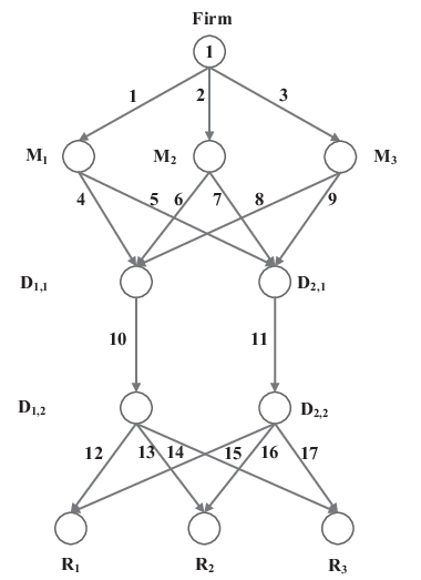
Consider the supply chain network shown in Fig. 1: a firm corresponding to node 1 aims at delivering the goods or products to the bottom level corresponding to the retail outlets. The links connecting the source node with the destination nodes represent the activities of production, storage and transportation of good or services. Different network topologies corresponds to different supply chain network problems. In this paper, we assume that there exists only one path linking node 1 with each destination node, which can ensure that the demand at each retail outlet can be satisfied.

As shown in Fig. 1, the firm takes into consideration $n_{M}$ manufacturers, $n_{D}$ distribution centers when $n_{R}$ retailers with demands ${d_{{R_{1}}}},{d_{{R_{2}}}},\cdots,{d_{{R_{{n_{R}}}}}}$ must be served. The node $1$ in the first layer is linked with the possible $n_{M}$ manufacturers, which are represented as ${M_{1}},{M_{2}},\cdots,{M_{{n_{M}}}}$. These edges in the manufacturing level are associated with the possible distribution center nodes, which are expressed by ${D_{1,1}},{D_{2,1}},\cdots,{D_{{n_{D}},1}}$. These links mean the possible shipment between the manufacturers and the distribution centers. The links connecting ${D_{1,1}},{D_{2,1}},\cdots,{D_{{n_{D}},1}}$ with ${D_{1,2}},{D_{2,2}},\cdots,{D_{{n_{D}},2}}$ reflect the possible storage links. The links between ${D_{1,2}},{D_{2,2}},\cdots,{D_{{n_{D}},2}}$ and ${R_{1}},{R_{1}},\cdots,{R_{{n_{R}}}}$ denote the possible shipment links connecting the storage centers with the retail outlets.

Let a supply chain network be represented by a graph $G(N,L)$, where $N$ is a set of nodes and $L$ is a set of links. Each links in the network is associated with a cost function and the cost reflects the total cost of all the specific activities in the supply chain network, such as the transport of the product, the delivery of the product, etc. The cost related with link $a$ is expressed by ${\widehat{c}_{a}}$. A path $p$ connecting node 1 with a retail node shown in Fig. 1 denotes the whole activities related with manufacturing the products, storing them and transporting them, etc. Assume $w_{k}$ denotes the set of source and destination nodes $(1,R_{k})$ and $P_{w_{k}}$ represents the set of alternative associated possible supply chain network processes joining $(1,R_{k})$. Then $P$ means the set of all paths joining $(1,R_{k})$ while $x_{p}$ denotes the flow of the product on path $p$, then the following Eq. (1) must be satisfied:

Let $f_{a}$ represent the flow on link $a$, then the following conservation flow must be met:

Eq. (2) means that the inflow must be equal to the outflow on link $a$.

These flows can be grouped into the vector $f$. The flow on each link must be a nonnegative number, i.e. the following Eq. (5) must be satisfied:

Suppose the maximum capacity on link $a$ is expressed by $u_{a},\forall a\in L$. It is required that the actual flow on link $a$ cannot exceed the maximum capacity on this link:

The total cost on each link, for the simplicity, they can be represented as a function of the flow of the product on all the links [32, 30, 33, 34]:

The total investment cost of adding capacity $u_{a}$ on link $a$ can be expressed as follows:

Summarily, the supply chain network design optimization problem is to satisfy the demand of each retail outlet and minimize the total cost, including the total cost of operating the various links and the capacity investments:

subject to constraints (1)-(4).

Physarum Polycephalum is a large, single-celled amoeboid organism forming a dynamic tubular network connecting the discovered food sources during foraging. The mechanism of tube formation can be described as follows. Tubes thicken in a given direction when shuttle streaming of the protoplasm persists in that direction for a certain time. There is a positive feedback between flux and tube thickness, as the conductance of the sol is greater in a thicker channel. With this mechanism in mind, a mathematical model illustrating the shortest path finding has been constructed [35].

Suppose the shape of the network formed by the Physarum is represented by a graph, in which a plasmodial tube refers to an edge of the graph and a junction between tubes refers to a node. Two special nodes labeled as $N_{1}$, $N_{2}$ act as the starting node and ending node respectively. The other nodes are labeled as $N_{3},N_{4},N_{5},N_{6}$ etc. The edge between nodes $N_{i}$ and $N_{j}$ is $M_{ij}$. The parameter $Q_{ij}$ denotes the flux through tube $M_{ij}$ from node $N_{i}$ to $N_{j}$. Assume the flow along the tube is approximated by Poiseuille flow. Then the flux ${Q_{ij}}$ can be expressed as:

where ${p_{i}}$ is a pressure at a node ${N_{i}}$, ${D_{ij}}$ is a conductivity of a tube ${M_{ij}}$, and $L_{ij}$ is its length.

By assuming that the inflow and outflow must be balanced, we have:

For the source node ${N_{1}}$ and the sink node ${N_{2}}$ the following holds:

where ${I_{0}}$ is the flux flowing from the source node and ${I_{0}}$ is a constant value here.

In order to describe such an adaptation of tubular thickness we assume that the conductivity ${D_{ij}}$ changes over time according to the flux ${Q_{ij}}$. An evolution of ${D_{ij}(t)}$ can be described by the following equation:

where $r$ is a decay rate of the tube. The equation implies that a conductivity becomes nil if there is no flux along the edge. The conductivity increases with the flux. The $f$ is monotonically increasing continuous function satisfying $f(0)=0$.

Then the network Poisson equation for the pressure can be obtained from the Eq. (8-11) as follows:

By setting ${p_{2}}$=0 as a basic pressure level, all ${p_{i}}$ can be determined by solving Eq. (13) and ${Q_{ij}}$ can also be obtained.

In this paper, $f(Q)=|Q|$ is used because $f\left({\left|{{Q_{ij}}}\right|}\right)=\left|Q\right|,\gamma=1$, the Physarum converges to the shortest path with a high rate [35]. With the flux calculated, the conductivity can be derived, where Eq. (14) is used instead of Eq. (12), adopting the functional form $f(Q)=|Q|$.

In the original Physarum model [35], there is only one source node and one ending node. In the supply chain network design problem, as shown in Fig. 1, there are $R_{n_{R}}$ retail outlets. From left to right, from top to bottom, we can number the nodes shown in Fig. 1. As a result, the following Eq. (15) is formulated to replace the Eq. (13).

where $j=1$ means that $\sum\limits_{i=1}^{n_{R}}{{d_{{R_{i}}}}}$ units of goods are distributed from the firm to the other manufacturing facilities, $j=R_{{n_{R}}}$ denotes $n_{R}$ retail outlet needs $d_{R_{j}}$ units of goods.

In the original Physarum model, the length associated with each link is fixed. In the supply chain network design problem, the cost on each link, be it a production link, a shipment link, or a storage link, is comprised of the cost of the flow on each link ${\widehat{c}_{a}}\left(f\right)$ and the investment cost ${\widehat{\pi}_{a}}\left({{u_{a}}}\right)$. Practically, the flow on each link should be equal to its capacity. Assume there is flow $f_{ij}$ passing through the link $(i,j)$, we take the following measure to convert the two costs into one.

As a result, Eq. (16) will be updated as below:

where $f_{ij}$ represents the flow on the link starting from node $i$ to node $j$.

In the Physarum model, it is necessary for us to initialize the related parameters, including the link length $L$, the conductivity $D$, and the pressure $Q$ at each node. In the supply chain network design model, the capacity and the flow are the unknown design variables. If we don’t know the specific flow on each link, we cannot determine its cost, which further leads to the initialization failure of Physarum algorithm. To prevent this failure we initialize the length on each link as a very small value ranging from 0.01 to 0.0001.

To satisfy the imposed capacity on each link, we bring in a new parameter called Capacity Ratio (CR). Let $f_{ij}$ be a flow on link $(i,j)$ is $f_{ij}$ then the imposed capacity on link $(i,j)$ is represented as $u_{ij}$. The CR associated with this link is defined as follows:

By defining this parameter, we aim at updating the cost on link $(i,j)$ as below:

In this process, the parameter CR has an important role from two aspects. On the one hand, if the flow $f_{ij}$ exceeds its capacity $u_{ij}$, then $CR_{ij}$ will be bigger than 1, which leads to the increase of $L_{ij}$. Otherwise, $CR_{ij}$ will be less than 1, which further results in the decrease of $L_{ij}$.

According to the mechanism lying in the Physarum model, every time the links’ length changes, the flow along each link is reallocated adaptively. Bonifaci et al. [36] has proved that the mass of the mould eventually converges to the shortest path. Based on this rule, after a series of reallocation, we can reach the equilibrium state in the supply chain network design problem and the optimal supply chain network can be obtained.

The main flow of Physarum model is presented in Algorithm 1. The firm and the retail outlets are treated as the starting node and the ending node, respectively.

First of all, the conductivity of each tube (Dij) is initiated with random value between $0$ and $1$ and other variables are assigned with $0$, including flux through each tube ($Q_{ij}$), pressure at each node ($P_{i}$).

Secondly, we can obtain the pressure associated with each node using Eq. (17). Besides, the flux passing through each link and the conductivity in the next iteration can be recorded. Thirdly, we will update the cost on each link using Eq. (16). In order to satisfy the capacity constraint, Eq. (19) is imposed.

There are several possible solutions to decide when to stop execution of Algorithm 1, such as the maximum number of iterations is arrived, conductivity of each tube converges to 0 or 1, flux through each tube remains unchanged, etc. The algorithm described in present paper halts when $\sum\limits_{i=1}^{N}{\sum\limits_{j=1}^{N}{\left|{D_{ij}^{n}-D_{ij}^{n-1}}\right|}}\leq\delta$, where $\delta$ is a threshold value.

References

- [1] Z. Liu, A. Nagurney, Supply chain networks with global outsourcing and quick-response production under demand and cost uncertainty, Annals of Operations Research 208 (1) (2013) 251–289.
- [2] W. Zhang, D. Xu, Integrating the logistics network design with order quantity determination under uncertain customer demands, Expert Systems with Applications 41 (1) (2014) 168–175.
- [3] M. Yu, A. Nagurney, Competitive food supply chain networks with application to fresh produce, European Journal of Operational Research 224 (2) (2013) 273–282.
- [4] H. Ma, C. Suo, A model for designing multiple products logistics networks, International Journal of Physical Distribution & Logistics Management 36 (2) (2006) 127–135.
- [5] T. Santoso, S. Ahmed, M. Goetschalckx, A. Shapiro, A stochastic programming approach for supply chain network design under uncertainty, European Journal of Operational Research 167 (1) (2005) 96–115.
- [6] G. Zhou, H. Min, M. Gen, The balanced allocation of customers to multiple distribution centers in the supply chain network: a genetic algorithm approach, Computers & Industrial Engineering 43 (1) (2002) 251–261.
- [7] P. Trkman, K. McCormack, Supply chain risk in turbulent environments¡ªA conceptual model for managing supply chain network risk, International Journal of Production Economics 119 (2) (2009) 247–258.
- [8] F. Altiparmak, M. Gen, L. Lin, I. Karaoglan, A steady-state genetic algorithm for multi-product supply chain network design, Computers & Industrial Engineering 56 (2) (2009) 521–537.
- [9] A. Ahmadi Javid, N. Azad, Incorporating location, routing and inventory decisions in supply chain network design, Transportation Research Part E: Logistics and Transportation Review 46 (5) (2010) 582–597.
- [10] A. Nagurney, Supply chain network design under profit maximization and oligopolistic competition, Transportation Research Part E: Logistics and Transportation Review 46 (3) (2010a) 281–294.
- [11] B. Bilgen, Application of fuzzy mathematical programming approach to the production allocation and distribution supply chain network problem, Expert Systems with Applications 37 (6) (2010) 4488–4495.
- [12] B. M. Beamon, Supply chain design and analysis::: Models and methods, International journal of production economics 55 (3) (1998) 281–294.
- [13] R. B. Handfield, E. L. Nichols, Supply chain redesign: Transforming supply chains into integrated value systems, FT Press, 2002.
- [14] A. Nagurney, Optimal supply chain network design and redesign at minimal total cost and with demand satisfaction, International Journal of Production Economics 128 (1) (2010b) 200–208.
- [15] S. L. Stephenson, H. Stempen, I. Hall, Myxomycetes: a handbook of slime molds, Timber Press Portland, Oregon, 1994.
- [16] T. Nakagaki, H. Yamada, Á. Tóth, Intelligence: Maze-solving by an amoeboid organism, Nature 407 (6803) (2000) 470–470.
- [17] X. Zhang, Z. Zhang, Y. Zhang, D. Wei, Y. Deng, Route selection for emergency logistics management: A bio-inspired algorithm, Safety Science 54 (2013a) 87–91.
- [18] X. Zhang, Q. Wang, F. T. S. Chan, S. Mahadevan, Y. Deng, A Physarum Polycephalum Optimization Algorithm for the Bi-objective Shortest Path Problem., International Journal of Unconventional Computing 10 (1-2) (2014) 143–162.
- [19] A. Tero, R. Kobayashi, T. Nakagaki, Physarum solver: A biologically inspired method of road-network navigation, Physica A: Statistical Mechanics and its Applications 363 (1) (2006) 115–119.
- [20] X. Zhang, S. Huang, Y. Hu, Y. Zhang, S. Mahadevan, Y. Deng, Solving 0-1 knapsack problems based on amoeboid organism algorithm, Applied Mathematics and Computation 219 (19) (2013b) 9959–9970.
- [21] Y. Zhang, Z. Zhang, Y. Deng, S. Mahadevan, A biologically inspired solution for fuzzy shortest path problems, Applied Soft Computing 13 (5) (2013c) 2356–2363.
- [22] T. Nakagaki, M. Iima, T. Ueda, Y. Nishiura, T. Saigusa, A. Tero, R. Kobayashi, K. Showalter, Minimum-risk path finding by an adaptive amoebal network, Physical Review Letters 99 (6) (2007) 068104.
- [23] A. I. Adamatzky, Route 20, Autobahn 7, and Slime Mold: Approximating the Longest Roads in USA and Germany With Slime Mold on 3-D Terrains., IEEE Transactions on Cybernetics .
- [24] A. Tero, K. Yumiki, R. Kobayashi, T. Saigusa, T. Nakagaki, Flow-network adaptation in Physarum amoebae, Theory in Biosciences 127 (2) (2008) 89–94.
- [25] A. Tero, S. Takagi, T. Saigusa, K. Ito, D. P. Bebber, M. D. Fricker, K. Yumiki, R. Kobayashi, T. Nakagaki, Rules for biologically inspired adaptive network design, Science 327 (5964) (2010) 439–442.
- [26] A. Adamatzky, Bioevaluation of World Transport Networks, World Scientific, 2012.
- [27] A. Adamatzky, G. J. Martínez, S. V. Chapa-Vergara, R. Asomoza-Palacio, C. R. Stephens, Approximating Mexican highways with slime mould, Natural Computing 10 (3) (2011) 1195–1214.
- [28] A. Adamatzky, Physarum machines: computers from slime mould, vol. 74, World Scientific, 2010.
- [29] A. Adamatzky, T. Schubert, Slime mold microfluidic logic gates, Materials Today 17 (2) (2014) 86–91.
- [30] A. Nagurney, A system-optimization perspective for supply chain network integration: The horizontal merger case, Transportation Research Part E: Logistics and Transportation Review 45 (1) (2009) 1–15.
- [31] A. Nagurney, T. Woolley, Q. Qiang, Multi-product supply chain horizontal network integration: models, theory, and computational results, International Transactions in Operational Research 17 (3) (2010) 333–349.
- [32] A. Nagurney, Supply chain network economics: dynamics of prices, flows and profits, Edward Elgar Publishing, 2006.
- [33] A. Nagurney, J. Dong, D. Zhang, A supply chain network equilibrium model, Transportation Research Part E: Logistics and Transportation Review 38 (5) (2002) 281–303.
- [34] A. Nagurney, T. Woolley, Environmental and cost synergy in supply chain network integration in mergers and acquisitions, in: Multiple Criteria Decision Making for Sustainable Energy and Transportation Systems, Springer, 57–78, 2010.
- [35] A. Tero, R. Kobayashi, T. Nakagaki, A mathematical model for adaptive transport network in path finding by true slime mold, Journal of Theoretical Biology 244 (4) (2007) 553–564.
- [36] V. Bonifaci, K. Mehlhorn, G. Varma, Physarum can compute shortest paths, Journal of Theoretical Biology 309 (2012) 121–133.