The old nuclear star cluster in the Milky Way: dynamics, mass, statistical parallax, and black hole mass
Abstract
We derive new constraints on the mass, rotation, orbit structure and statistical parallax of the Galactic old nuclear star cluster and the mass of the supermassive black hole. We combine star counts and kinematic data from Fritz et al. (2014), including 2’500 line-of-sight velocities and 10’000 proper motions obtained with VLT instruments. We show that the difference between the proper motion dispersions and cannot be explained by rotation, but is a consequence of the flattening of the nuclear cluster. We fit the surface density distribution of stars in the central by a superposition of a spheroidal cluster with scale and a much larger nuclear disk component. We compute the self-consistent two-integral distribution function for this density model, and add rotation self-consistently. We find that: (i) The orbit structure of the gives an excellent match to the observed velocity dispersion profiles as well as the proper motion and line-of-sight velocity histograms, including the double-peak in the -histograms. (ii) This requires an axial ratio near consistent with our determination from star counts, for . (iii) The nuclear star cluster is approximately described by an isotropic rotator model. (iv) Using the corresponding Jeans equations to fit the proper motion and line-of-sight velocity dispersions, we obtain best estimates for the nuclear star cluster mass, black hole mass, and distance , , and kpc, where the estimated systematic errors account for additional uncertainties in the dynamical modeling. (v) The combination of the cluster dynamics with the S-star orbits around Sgr A∗ strongly reduces the degeneracy between black hole mass and Galactic centre distance present in previous S-star studies. A joint statistical analysis with the results of Gillessen et al. (2009) gives and kpc.
Keywords:
galaxy center, nuclear cluster, kinematics and dynamics.1 INTRODUCTION
Nuclear star clusters (NSC) are located at the centers of most spiral galaxies (Carollo et al., 1997; Böker et al., 2002). They are more luminous than globular clusters (Böker et al., 2004), have masses of order (Walcher et al., 2005), have complex star formation histories (Rossa et al., 2006; Seth et al., 2006), and obey scaling-relations with host galaxy properties as do central supermassive black holes (Ferrarese et al., 2006; Wehner & Harris, 2006, SMBH;); see Böker (2010) for a review. Many host an AGN, i.e., a SMBH (Seth et al., 2008), and the ratio of NSC to SMBH mass varies widely (Graham & Spitler, 2009; Kormendy & Ho, 2013).
The NSC of the Milky Way is of exceptional interest because of its proximity, about 8 kpc from Earth. It extends up to several hundred arcsecs from the center of the Milky Way (Sgr A*) and its mass within 1 pc is with uncertainty (Schödel et al., 2009; Genzel et al., 2010). There is strong evidence that the center of the NSC hosts a SMBH of several million solar masses. Estimates from stellar orbits show that the SMBH mass is (Schödel et al., 2002; Ghez et al., 2008; Gillessen et al., 2009). Due to its proximity, individual stars can be resolved and number counts can be derived; however, due to the strong interstellar extinction the stars can only be observed in the infrared. A large number of proper motions and line-of-sight velocities have been measured, and analyzed with spherical models to attempt to constrain the NSC dynamics and mass (Haller et al., 1996; Genzel et al., 1996; Genzel et al., 2000; Trippe et al., 2008; Schödel et al., 2009; Fritz et al., 2014).
The relaxation time of the NSC within 1 pc is yr (Alexander, 2005; Merritt, 2013), indicating that the NSC is not fully relaxed and is likely to be evolving. One would expect from theoretical models that, if relaxed, the stellar density near the SMBH should be steeply-rising and form a Bahcall & Wolf (1976) cusp. In contrast, observations by Do et al. (2009); Buchholz et al. (2009); Bartko et al. (2010) show that the distribution of old stars near the SMBH appears to have a core. Understanding the nuclear star cluster dynamics may therefore give useful constraints on the mechanisms by which it formed and evolved (Merritt, 2010).
In this work we construct axisymmetric Jeans and two-integral distribution function models based on stellar number counts, proper motions, and line-of-sight velocities. We describe the data briefly in Section 2; for more detail the reader is referred to the companion paper of Fritz et al. (2014). In Section 3 we carry out a preliminary study of the NSC dynamics using isotropic spherical models, in view of understanding the effect of rotation on the data. In Section 4 we describe our axisymmetric models and show that they describe the kinematic properties of the NSC exceptionally well. By applying a minimization algorithm, we estimate the mass of the cluster, the SMBH mass, and the NSC distance. We discuss our results and summarize our conclusions in Section 5. The Appendix contains some details on our use of the Qian et al. (1995) algorithm to calculate the two-integral distribution function for the fitted density model.
2 DATASET
We first give a brief description of the data set used for our dynamical analysis. These data are taken from Fritz et al. (2014) and are thoroughly examined in that paper, which should be consulted for more details. The coordinate system used is a shifted Galactic coordinate system () where Sgr A* is at the center and () are parallel to Galactic coordinates (). In the following we always refer to the shifted coordinates but will omit the asterisks for simplicity. The dataset consists of stellar number densities, proper motions and line-of-sight velocities. We use the stellar number density map rather than the surface brightness map because it is less sensitive to individual bright stars and non-uniform extinction.
The stellar number density distribution is constructed from NACO high-resolution images for , in a similar way as in Schödel et al. (2010), from HST WFC3/IR data for , and from VISTA-VVV data for .
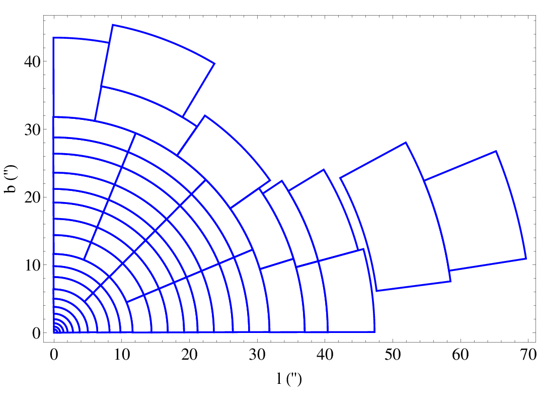
The kinematic data include proper motions for 10’000 stars obtained from AO assisted images. The proper motion stars are binned into 58 cells (Fritz et al., 2014, Figure 1;) according to distance from Sgr A* and the Galactic plane. This binning assumes that the NSC is symmetric with respect to the Galactic plane and with respect to the -axis on the sky, consistent with axisymmetric dynamical modeling. The sizes of the bins are chosen such that all bins contain comparable numbers of stars, and the velocity dispersion gradients are resolved, i.e., vary by less than the error bars between adjacent bins.
Relative to the large velocity dispersions at the Galactic center (100 km/s), measurement errors for individual stars are typically , much smaller than in typical globular cluster proper motion data where they can be (e.g., in Omega Cen; van de Ven et al. (2006)). Therefore corrections for these measurement errors are very small.
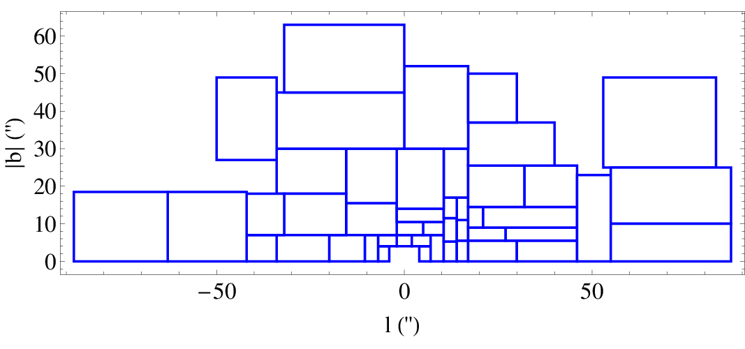
We also use 2’500 radial velocities obtained from SINFONI integral field spectroscopy. The binning of the radial velocities is shown in Fig. 2. There are 46 rectangular outer bins as shown in Fig. 2 plus 6 small rectangular rings around the center (Fritz et al., 2014, not shown; see App. E of). Again the outer bins are chosen such that they contain similar numbers of stars and the velocity dispersion gradients are resolved. The distribution of radial velocity stars on the sky is different from the distribution of proper motion stars, and it is not symmetric with respect to . Because of this and the observed rotation, the binning is different, and extends to both positive and negative longitudes. Both the proper motion and radial velocity binning are also used in Fritz et al. (2014) and some tests are described in that paper.
Finally, we compare our models with (but do not fit to) the kinematics derived from about 200 maser velocities at (Lindquist et al., 1992; Deguchi et al., 2004, from). As for the proper motion and radial velocity bins, we use the mean velocities and velocity dispersions as derived in Fritz et al. (2014).
The assumption that the NSC is symmetric with respect to the Galactic plane and the axis is supported by the recent Spitzer/IRAC photometry (Schödel et al., 2014) and by the distribution of proper motions (Fritz et al., 2014). The radial velocity data at intermediate radii instead show an apparent misalignment with respect to the Galactic plane, by ; see Feldmeier et al. (2014) and Fritz et al. (2014). We show in Section 4.2 that, even if confirmed, such a misaligned structure would have minimal impact on the results obtained here with the symmetrised analysis.
3 SPHERICAL MODELS OF THE NSC
In this section we study the NSC using the preliminary assumption that the NSC can be described by an isotropic distribution function (DF) depending only on energy. We use the DF to predict the kinematical data of the cluster. Later we add rotation self-consistently to the model. The advantages of using a distribution function instead of common Jeans modeling are that (i) we can always check if a DF is positive and therefore if the model is physical, and (ii) the DF provides us with all the moments of the system. For the rest of the paper we use for spherical and for cylindrical coordinates, with corresponding to the z-axis normal to the equatorial plane of the NSC.
3.1 Mass model for the NSC
The first step is to model the surface density. We use the well-known one-parameter family of spherical -models (Dehnen, 1993):
| (1) |
where is the scaling radius and the total mass.The model behaves as for and for . Dehnen models are equivalent to the -models of Tremaine et al. (1994) under the transformation . Special cases are the Jaffe (1983) and Hernquist (1990) models for and respectively. For the model approximates de Vaucouleurs law. In order to improve the fitting of the surface density we use a combination of two -models, i.e.
| (2) |
The use of a two-component model will prove convenient later when we move to the axisymmetric case. The projected density is
| (3) |
and can be expressed in terms of elementary functions for integer , or in terms of elliptic integrals for half-integer . For arbitrary and the surface density can only be calculated numerically using equation (3). The surface density diverges for but is finite for .
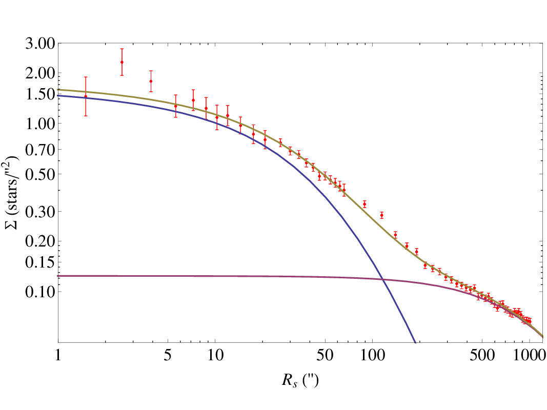
The projected number density profile of the NSC obtained from the data of Fritz et al. (2014) (see Section 2) is shown in Figure 3. The inflection point at indicates that the NSC is embedded in a more extended, lower-density component. The surface density distribution can be approximated by a two-component model of the form of equation (2), where the six parameters are fitted to the data subject to the following constraints: The slope of the inner component should be because isotropic models with a black hole and are unphysical (Tremaine et al., 1994), but it should be close to the limiting value of 0.5 to better approximate the observed core near the center (Buchholz et al., 2009). For the outer component so that it is negligible in the inner part of the density profile. In addition and . With these constraints we start with some initial values for the parameters and then iteratively minimize . The reduced resulting from this procedure is for d.o.f. and the corresponding best-fit parameter values are:
Here we provide only the ratio of masses instead of absolute values in model units since the shape of the model depends only on the ratio. The surface density of the final model is overplotted on the data in Figure 3.
3.2 Spherical model
With the assumption of constant mass-to-light ratio and the addition of the black hole the potential () will be (Dehnen, 1993)
| (6) |
where is the mass of the black hole. Since we now know the potential and the density we can calculate the distribution function (DF) numerically using Eddington’s formula, as a function of positive energy ,
| (7) |
The 2nd term of the equation vanishes for reasonable behavior of the potential and the double derivative inside the integral can be calculated easily by using the transformation
| (8) |
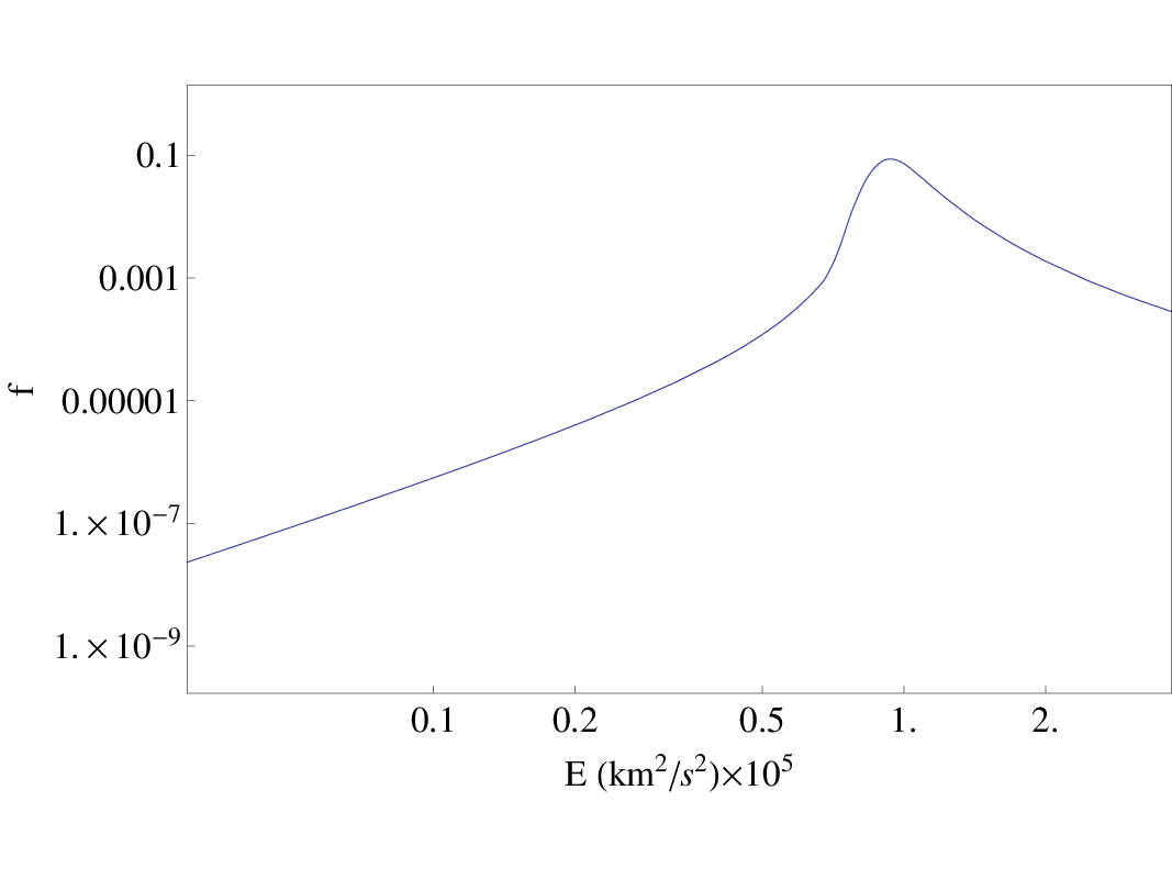
Figure 4 shows the DF of the two components in their joint potential plus that of a black hole with mass ratio . The DF is positive for all energies. We can test the accuracy of the DF by retrieving the density using
| (9) |
and comparing it with equation (2). Both agree to within . The DF has the typical shape of models with a shallow cusp of . It decreases as a function of energy both in the neighborhood of the black hole and also for large energies. It has a maximum near the binding energy of the stellar potential well (Baes et al., 2005).
For a spherical isotropic model the velocity ellipsoid (Binney & Tremaine, 2008) is a sphere of radius . The intrinsic dispersion can be calculated directly using
| (10) |
The projected dispersion is then given by:
| (11) |
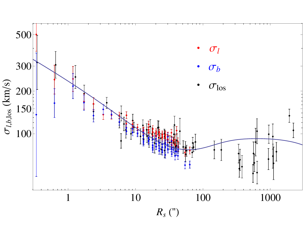
In Figure 5 we see how our two-component model compares with the kinematical data using the values kpc for the distance to the Galactic centre, for the black hole mass, and for the cluster mass inside 100”. The good match of the data up to suggests that the assumption of constant mass-to-light ratio for the cluster is reasonable. Later-on we will see that a flattened model gives a much better match also for the maser data.
3.3 Adding self-consistent rotation to the spherical model
We describe here the effects of adding self-consistent rotation to the spherical model, but much of this also applies to the axisymmetric case which will be discussed in Section 4. We assume that the rotation axis of the NSC is aligned with the rotation axis of the Milky Way disk. We also use a cartesian coordinate system where is parallel to the axis of rotation as before, is along the line of sight, and is along the direction of negative longitude, with the center of the NSC located at the origin. The proper motion data are given in Galactic longitude and Galactic latitude angles, but because of the large distance to the center, we can assume that and .
Whether a spherical system can rotate has been answered in Lynden Bell (1960). Here we give a brief review. Rotation in a spherical or axisymmetric system can be added self-consistently by reversing the sense of rotation of some of its stars. Doing so, the system will remain in equilibrium. This is equivalent with adding to the DF a part that is odd with respect to . The addition of an odd part does not affect the density (or the mass) because the integral of the odd part over velocity space is zero. The most effective way to add rotation to a spherical system is by reversing the sense of rotation of all of its counterrotating stars. This corresponds to adding (Lynden Bell, 1960, Maxwell’s daemon,) to the initially non-rotating DF, and generates a system with the maximum allowable rotation. The general case of adding rotation to a spherical system can be written where is an odd function with to ensure positivity of the DF. We notice that the new distribution function is a three-integral DF. In this case the density of the system is still rotationally invariant but is not.
In Figure 5 we notice that the projected velocity dispersion in the direction is larger than the dispersion in the direction which was first found by Trippe et al. (2008). This is particularly apparent for distances larger than . A heuristic attempt to explain this difference was made in Trippe et al. (2008) where they imposed a rotation of the form along with their Jeans modeling, as a proxy for axisymmetric modeling. Here we show that for a self-consistent system the difference in the projected and dispersions cannot be explained by just adding rotation to the cluster.
Specifically, we show that adding an odd part to the distribution function does not change the proper motion dispersion . The dispersion along the axis is . Writing in spherical velocity components (see the beginning of this section for the notation),
| (12) |
we see that
The second term vanishes because is even in , and odd in , so that the integrand for all terms of is odd in at least one velocity variable. We also have
The first part is zero because is odd. The second part is different from zero; however when projecting along the line-of-sight this term also vanishes because is an even function of when the integration is in a direction perpendicular to the angular momentum direction. Hence the projected mean velocity is zero, and the velocity dispersion is unchanged.
An alternative way to see this is by making a particle realization of the initial DF (Aarseth et al., 1974, e.g.). Then we can add rotation by reversing the sign of of a percentage of particles using some probability function which is equivalent to changing the signs of and of those particles. will not be affected by the sign change and the averaged over the line-of-sight will be zero because for each particle at the front of the system rotating in a specific direction there will be another particle at the rear of the system rotating in the opposite direction. In this work we do not use particle models to avoid fluctuations due to the limited number of particles near the center.
For the odd part of the DF we choose the two-parameter function from Qian et al. (1995). This is a modified version of Dejonghe (1986) which was based on maximum entropy arguments:
| (17) |
where , is the maximum allowable value of at a given energy, and and are free parameters. The parameter F works as a global adjustment of rotation while the parameter determines the contributions of stars with different ratios. Specifically for small only stars with high will contribute while large implies that all stars irrespective of their contribute to rotation. For F=1 and , which corresponds to maximum rotation.
From the resulting distribution function we can calculate in cylindrical coordinates using the equation
| (18) |
To find the mean line-of-sight velocity versus Galactic longitude we have to project equation (18) to the sky plane
| (19) |
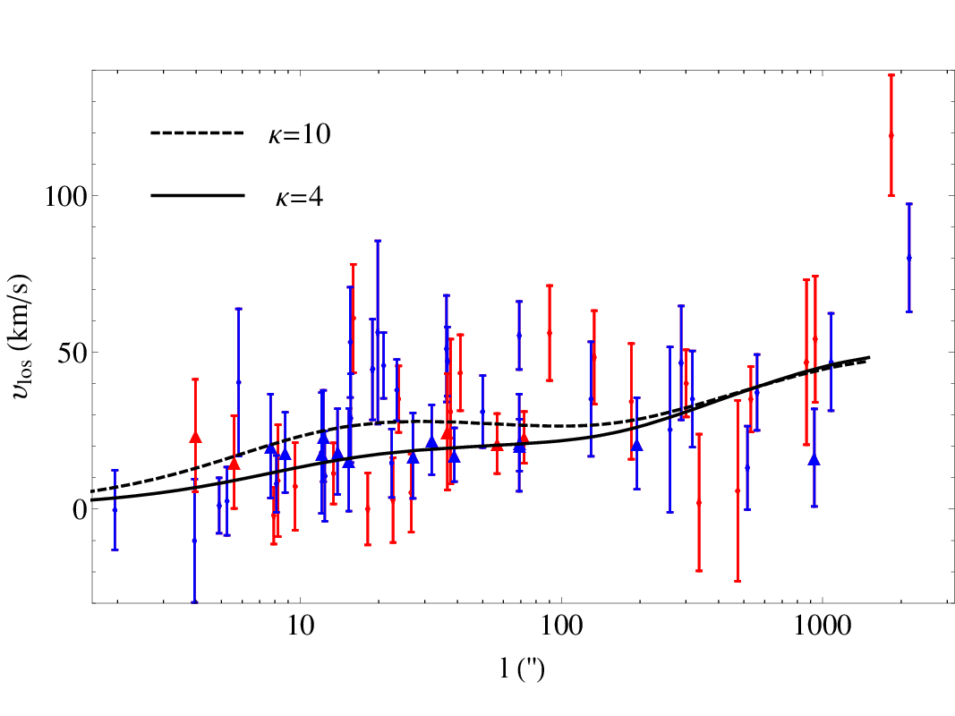
Figure 6 shows the mean line-of-sight velocity data vs Galactic longitude for and two values for the parameters in equation (17). Later in the axisymmetric section we constrain these parameters by fitting. Each data point corresponds to a cell from Figure 2. The maser data () are also included. The signs of velocities for negative are reversed because of the assumed symmetry. The line shows the prediction of the model with parameters determined with equation (19). Figure 2 shows that the line-of-sight velocity cells extend from b=0 to up to , but most of them lie between 0 and . For this reason we compute the model prediction at an average value of .
4 AXISYMMETRIC MODELING OF THE NSC
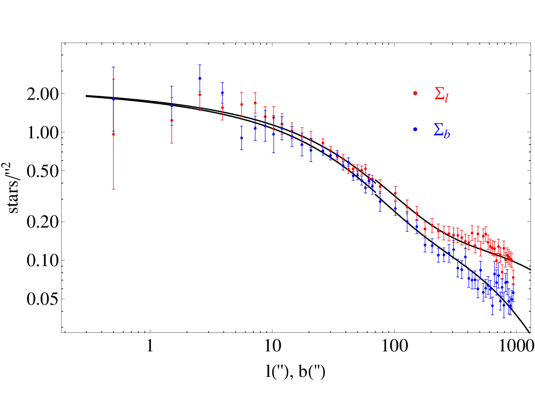
We have seen that spherical models cannot explain the difference between the velocity dispersions along the and directions. The number counts also show that the cluster is flattened; see Figure 7 and Fritz et al. (2014). Therefore we now continue with axisymmetric modeling of the nuclear cluster. The first step is to fit the surface density counts with an axisymmetric density model. The available surface density data extend up to in the and directions. For comparison, the proper motion data extend to from the centre (Figure 1). We generalize our spherical two-component -model from equation (2) to a spheroidal model given by
| (20) |
where is the spheroidal radius and the two new parameters are the axial ratios (prolate , oblate ) of the inner and outer component, respectively. Note that the method can be generalized to N components. The mass of a single component is given by . From Figure 7 we expect that the inner component will be more spherical than the outer component, although when the density profile gets flatter near the center it becomes more difficult to determine the axial ratio. In Figure 7 one also sees that the stellar surface density along the direction is larger than along the direction. Thus we assume that the NSC is an oblate system. To fit the model we first need to project the density and express it as a function of and . The projected surface density as seen edge on is
| (21) |
In general, to fit equation (21) to the data we would need to determine the eight parameters . However, we decided to fix a value for because the second component is not very well confined in the 8-dimensional parameter space (i.e. there are several models each with different and similar ). We choose , close to the value found in Fritz et al. (2014). For similar reasons, we also fix the value of to that used in the spherical case. The minimum value of for a semi-isotropic axisymmetric model with a black hole cannot be smaller than (Qian et al., 1995), as in the spherical case. For our current modeling we treat as a free parameter. Thus six free parameters remain. To fit these parameters to the data in Fig. 7 we apply a Markov chain Monte Carlo algorithm. For comparing the model surface density (21) to the star counts we found it important to average over angle in the inner conical cells to prevent an underestimation of the parameter. The values obtained with the MCMC algorithm for the NSC parameters and their errors are:
The reduced that corresponds to these parameter values is for d.o.f. Here we note that there is a strong correlation between the parameters and . The flattening of the inner component is very similar to the recent determination from Spitzer/IRAC photometry (Schödel et al., 2014, ,) but slightly more flattened than the best value given by Fritz et al. (2014), . The second component is about 100 times more massive than the first, but also extends more than one order of magnitude further.
Assuming constant mass-to-light ratio for the star cluster, we determine its potential using the relation from Qian et al. (1995), which is compatible with their contour integral method (i.e. it can be used for complex and ). The potential for a single component is given by:
| (25) |
with , , and where is the central potential (for a review of the potential theory of ellipsoidal bodies consider Chandrasekhar (1969)). The total potential of the two-component model is
| (26) |
4.1 Axisymmetric Jeans modeling
Here we first continue with axisymmetric Jeans modeling. We will need a large number of models to determine the best values for the mass and distance of the NSC, and for the mass of the embedded black hole. We will use DFs for the detailed modeling in Section 4.3, but this is computationally expensive, and so a large parameter study with the DF approach is not currently feasible. In Section 4.3 we will show that a two-integral (2I) distribution function of the form gives a very good representation to the histograms of proper motions and line-of-sight velocities for the nuclear star cluster in all bins. Therefore we can assume for our Jeans models that the system is semi-isotropic, i.e., isotropic in the meridional plane, . From the tensor virial theorem (Binney & Tremaine, 2008) we know that for 2I-models in order to produce the flattening. In principle, for systems of the form it is possible to find recursive expressions for any moment of the distribution function (Magorrian & Binney, 1994) if we know the potential and the density of the system. However, here we will confine ourselves to the second moments, since later we will recover the distribution function. By integrating the Jeans equations we get relations for the independent dispersions (Nagai & Miyamoto, 1976):
The potential and density are already known from the previous section. Once is found it can be used to calculate . The intrinsic dispersions in and direction are given by the equations:
where and . Projecting the previous equations along the line of sight we have:
where we note that the last quantity in (4.1) and (4.1) is the moment and not the line-of-sight velocity dispersion.
In order to define our model completely, we need to determine the distance and mass of the cluster and the black hole mass . To do this we apply a minimization technique matching all three velocity dispersions in both sets of cells, using the following procedure. First we note that the inclusion of self-consistent rotation to the model will not affect its mass. This means that for the fitting we can use for each cell of Figure 2. Similarly, since our model is axisymmetric we should match to the for each proper motion cell; the terms should be and indeed are negligible. Another way to see this is that since the system is axially symmetric, the integration of along the line-of-sight should be zero because the integration would cancel out for positive and negative .
With this in mind we proceed as follows, using the cluster’s density parameters11 1 It is computationally too expensive to simultaneously also minimize over the density parameters. as given in (4). First we partition the 3d space (, , ) into a grid with resolution . Then for each point of the grid we calculate the corresponding using the velocity dispersions from all cells in Figs. 1 and 2, excluding the two cells at the largest radii (see Fig. 8). We compare the measured dispersions with the model values obtained from equations (4.1) for the centers of these cells. Then we interpolate between the values on the grid and find the minimum of the interpolated function, i.e., the best values for (, , ). To determine statistical errors on these quantities, we first calculate the Hessian matrix from the curvature of surface at the minimum, . The statistical variances will be the diagonal elements of the inverted matrix.
With this procedure we obtain a minimum reduced with degrees of freedom, for the values
where
| (41) |
and the value given for in (4.1) is not the total cluster mass but the stellar mass within elliptical radius . In Section 4.2 we will consider in more detail the determination of these parameters and their errors. The model with density parameters as in (4) and dynamical parameters as in (4.1) will be our best model. In Section 4.3 we will see that it also gives an excellent prediction to the velocity histograms.
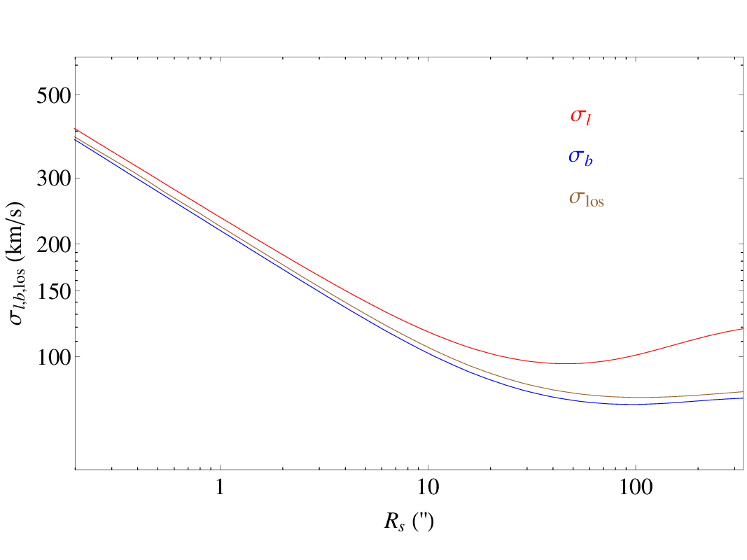
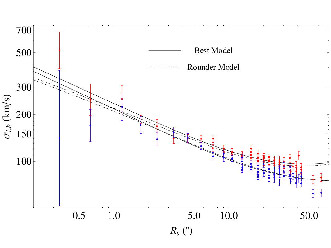
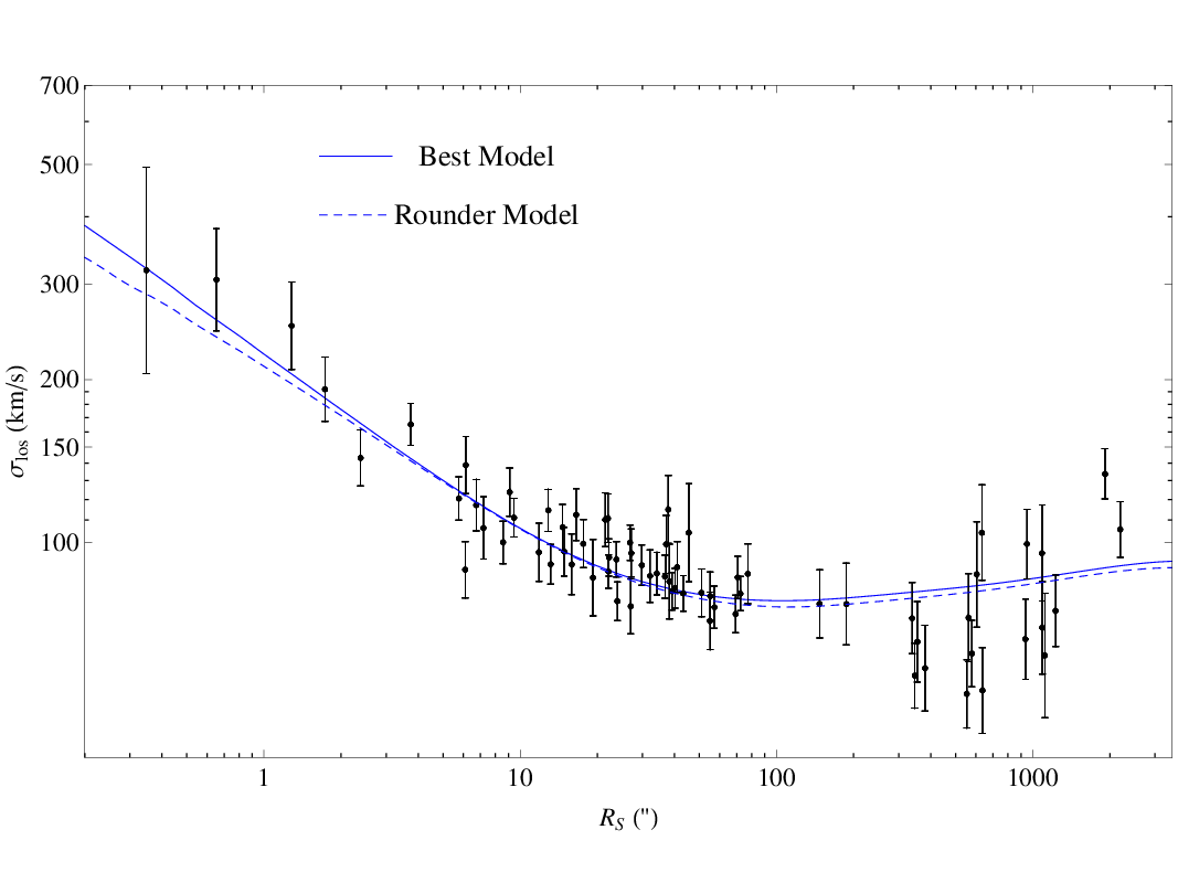
First, we now look at the comparison of this model with the velocity data. Figure 8 shows how the azimuthally averaged dispersions and compare with the measured proper motion dispersions. Figure 9 shows how this best model, similarly averaged, compares with the line-of-sight mean square velocity data. The maser data are also included in the plot. It is seen that the model fits the data very well, in accordance with its per cell. Figure 10 shows how all three projected dispersions of the model compare. is slightly lower than due to projection effects. The fact that all three velocity dispersion profiles in Figs. 8, 9 are fitted well by the model suggests that the assumed semi-isotropic dynamical structure is a reasonable approximation.
The model prediction in Fig. 8 is similar to Figure 11 of Trippe et al. (2008) but the interpretation is different. As shown in the previous section, the difference in projected dispersions cannot be explained by imposing rotation on the model. Here we demonstrated how the observational finding can be quantitatively reproduced by flattened axisymmetric models of the NSC and the surrounding nuclear disk.
Most of our velocity data are in the range 7”-70”, i.e., where the inner NSC component dominates the potential. In order to understand the dynamical implications of these data on the flattening of this component, we have also constructed several density models in which we fixed to values different from the obtained from star counts. In each case we repeated the fitting of the dynamical parameters as in (4.1). We found that models with in a range from to gave comparable fits () to the velocity dispersion data as our nominal best model but that a model with was noticeably worse. We present an illustrative model with flattening about half-way between the measured and the spherical case, for which we set . This is also close to the value given by (Fritz et al., 2014), . We simultaneously explore a slightly different inner slope, . We then repeat the fitting of the starcount density profile in Fig. 7 (model not shown), keeping also and fixed to the previous values, and varying the remaining parameters. Our rounder comparison model then has the following density parameters:
The best reduced that we obtain for the velocity dispersion profiles with these parameters is and corresponds to the values
Compared to the best and more flattened model, the cluster mass has increased and the black hole mass has decreased. The sum of both masses has changed only by and the distance only by . In Figures 8, 9 we see how the projected velocity dispersions of this model compare with our best model. The main difference seen in comes from the different flattening of the inner component, and the smaller slope of the dispersions near the center of the new model is because of its smaller central density slope.
4.2 Distance to the Galactic Center, mass of the star cluster, and mass of the black hole
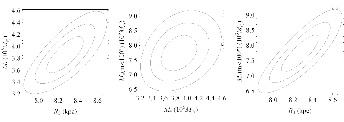
We now consider the determination of these parameters from the NSC data in more detail. Fig 11 shows the marginalized -plot for the NSC model as given in equation (4), for pairs of two parameters , , , as obtained from fitting the Jeans dynamical model to the velocity dispersion profiles. The figure shows contour plots for constant with , and in the three planes for the two-dimensional distribution of the respective parameters. We notice that the distance has the smallest relative error.
The best-fitting values for are given in equation (4.1); these values are our best estimates based on the NSC data alone. For the dynamical model with these parameters and the surface density parameters given in (4), the flattening of the inner component inferred from the surface density data is consistent with the dynamical flattening, which is largely determined by the ratio of and the tensor virial theorem.
Statistical errors are determined from the Hessian matrix for this model. Systematic errors can arise from uncertainties in the NSC density structure, from deviations from the assumed axisymmetric two-integral dynamical structure, from dust extinction within the cluster (see Section 5), and other sources. We have already illustrated the effect of varying the cluster flattening on with our second, rounder model. We have also tested how variations of the cluster density structure beyond impact the best-fit parameters, and found that these effects are smaller than those due to flattening variations.
We have additionally estimated the uncertainty introduced by the symmetrisation of the data if the misalignment found by Feldmeier et al. (2014); Fritz et al. (2014) were intrinsic to the cluster, as follows. We took all radial velocity stars and rotated each star by 10∘ clockwise on the sky. Then we resorted the stars into our radial velocity grid (Fig. 2). Using the new values obtained in the cells we fitted Jeans models as before. The values we found for , , with these tilted data differed from those in equation (4.1) by kpc, , and , respectively, which are well within the statistical errors.
Propagating the errors of the surface density parameters from the MCMC fit and taking into account the correlation of the parameters, we estimate the systematic uncertainties from the NSC density structure to be kpc in , in , and . We will see in Section 4.3 below that the DF for our illustrative rounder NSC model gives a clearly inferior representation of the velocity histograms than our best kinematic model, and also that the systematic differences between both models appear comparable to the residual differences between our preferred model and the observed histograms. Therefore we take the differences between these models, in , in , and in , as a more conservative estimate of the dynamical modeling uncertainties, so that finally
We note several other systematic errors which are not easily quantifiable and so are not included in these estimates, such as inhomogeneous sampling of proper motions or line-of-sight velocities, extinction within the NSC, and the presence of an additional component of dark stellar remnants.
Based on our best model, the mass of the star cluster within converted into spherical coordinates is . The model’s mass within the innermost pc () is in spheroidal radius, or in spherical radius. The total mass of the inner NSC component is . Because most of this mass is located beyond the radius where the inner component dominates the projected star counts, the precise division of the mass in the model between the NSC and the adjacent nuclear disk is dependent on the assumed slope of the outer density profile of NSC, and is therefore uncertain.
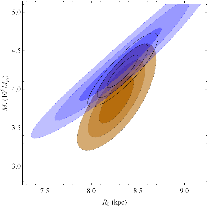
The distance and the black hole mass we found differ by and , respectively, from the values kpc and for kpc, as determined by Gillessen et al. (2009) from stellar orbits around Sgr A∗. Figure 12 shows the to contours of marginalized for jointly from stellar orbits (Gillessen et al., 2009), for the NSC model of this paper, and for the combined modeling of both data sets. The figure shows that both analyses are mutually consistent. When marginalized over and the respective other parameter, the combined modeling gives, for each parameter alone, kpc and . We note that these errors for and are both dominated by the distance error from the NSC modeling. Thus our estimated additional systematic error of kpc for in the NSC modeling translates to a similar additional error in the combined measurement and, through the SMBH mass-distance relation given in Gillessen et al (2009), to an additional uncertainty in . We see that the combination of the NSC and S-star orbit data is a powerful means for decreasing the degeneracy between the SMBH mass and Galactic center distance in the S-star analysis.
4.3 Two-integral distribution function for the NSC.
Now we have seen the success of fitting the semi-isotropic Jeans models to all three velocity dispersion profiles of the NSC, and determined its mass and distance parameters, we proceed to calculate two-integral (2I) distribution functions. We use the contour integral method of Hunter & Qian (1993, HQ) and Qian et al. (1995). A 2I DF is the logical, next-simplest generalization of isotropic spherical models. Finding a positive DF will ensure that our model is physical. Other possible methods to determine ) include reconstructing the DF from moments (Magorrian, 1995), using series expansions as in Dehnen & Gerhard (1994), or grid-based quadratic programming as in Kuijken (1995). We find the HQ method the most suitable since it is a straightforward generalization of Eddington’s formula. The contour integral is given by:
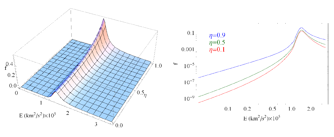
where . Equation (4.3) is remarkably similar to Eddington’s formula. Like in the spherical case the DF is even in . The integration for each pair takes place on the complex plane of the potential following a closed path (i.e. an ellipse) around the special value . For more information on the implementation and for a minor improvement over the original method see Appendix A. We find that a resolution of logarithmically placed cells in the space is adequate to give us relative errors of the order of when comparing with the zeroth moment, i.e., the density, already known analytically, and with the second moments, i.e., the velocity dispersions from Jeans modeling.
The gravitational potential is already known from equations (25) and (26). For the parameters (cluster mass, black hole mass, distance) we use the values given in (4.1). Figure 13 shows the DF in space. The shape resembles that of the spherical case (Fig. 4). The DF is a monotonically increasing function of and declines for small and large energies. The DF contains information about all moments and therefore we can calculate the projected velocity profiles (i.e., velocity distributions, hereafter abbreviated VPs) in all directions. The normalized VP in the line-of-sight (los) direction is
| (52) |
Using polar coordinates in the velocity space where and we find
| (53) |
where
and are the solutions of . Following a similar path we can easily find the corresponding integrals for the VPs in the and directions.
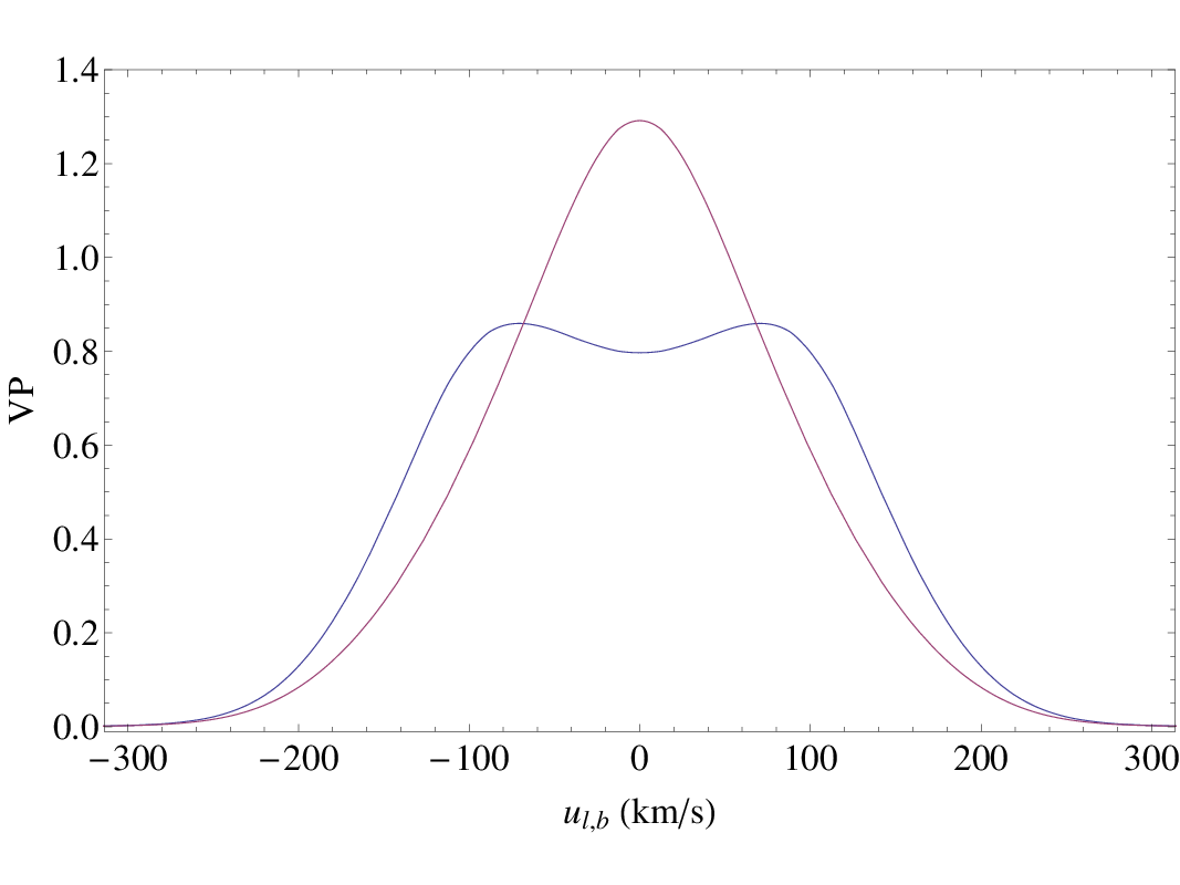
The typical shape of the VPs in the and directions within the area of interest is shown in Figure 14. We notice the characteristic two-peak shape of the VP along that is caused by the near-circular orbits of the flattened system. Because the front and the back of the axisymmetric cluster contribute equally, the two peaks are mirror-symmetric, and adding rotation would not change their shapes.
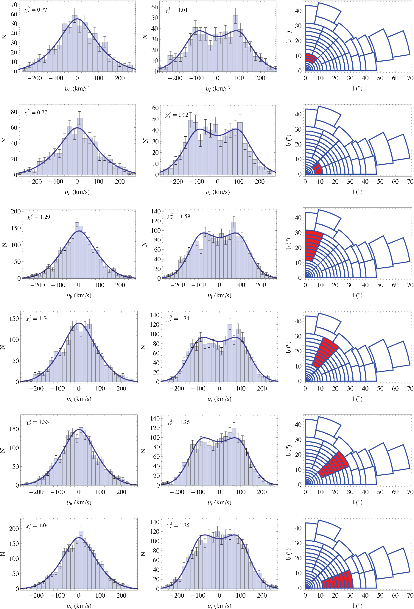
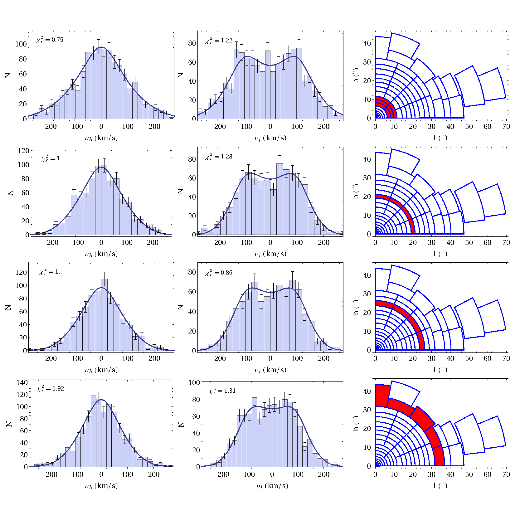
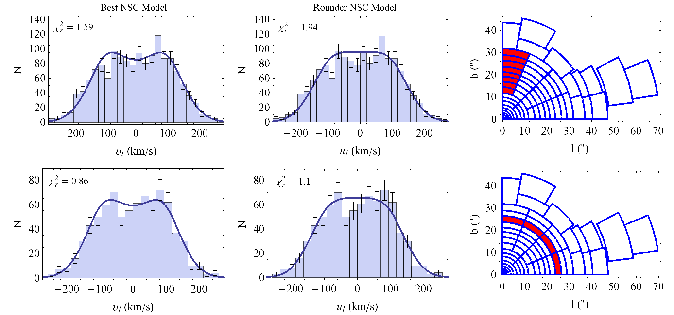
The middle panels of Figure 15 and Figures 21 and 22 in Appendix B show how our best model (with parameters as given in (4) and (4.1)) predicts the observed velocity histograms for various combinations of cells. The reduced for each histogram is also provided. The prediction is very good both for the VPs in and . Specifically, for the proper motions our flattened cluster model predicts the two-peak structure of the data pointed out by several authors (Trippe et al., 2008; Schödel et al., 2009; Fritz et al., 2014). In order to calculate the VP from the model for each cell we averaged over the VP functions for the center of each cell weighted by the number of stars in each cell and normalized by the total number of stars in all the combined cells.
Figure 15 compares two selected -VPs for our two main models with the data. The left column shows how the observed velocity histograms (VHs) for corresponding cells compare to the model VPs for the less flattened model with parameters given in (4.1) and (4.1), the middle column compares with the same VPs from our best model with parameters given in (4) and (4.1). Clearly, the more flattened model with fits the shape of the data much better than the more spherical model with , justifying its use in Section 4.2.
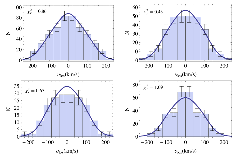
This model is based on an even DF in and therefore does not yet have rotation. To include rotation, we will (in Section 4.4) add an odd part to the DF, but this will not change the even parts of the model’s VPs. Therefore, we can already see whether the model is also a good match to the observed los velocities by comparing it to the even parts of the observed los VHs. This greatly simplifies the problem since we can think of rotation as independent, and can therefore adjust it to the data as a final step. Figure 23 shows how the even parts of the VHs from the los data compare with the VPs of the 2I model. Based on the reduced , the model provides a very good match. Possible systematic deviations are within the errors. The los VHs are broader than those in the direction because the los data contain information about rotation (the broader the even part of the symmetrized los VHs, the more rotation the system possesses, and in extreme cases they would show two peaks).
4.4 Adding rotation to the axisymmetric model: is the NSC an isotropic rotator?
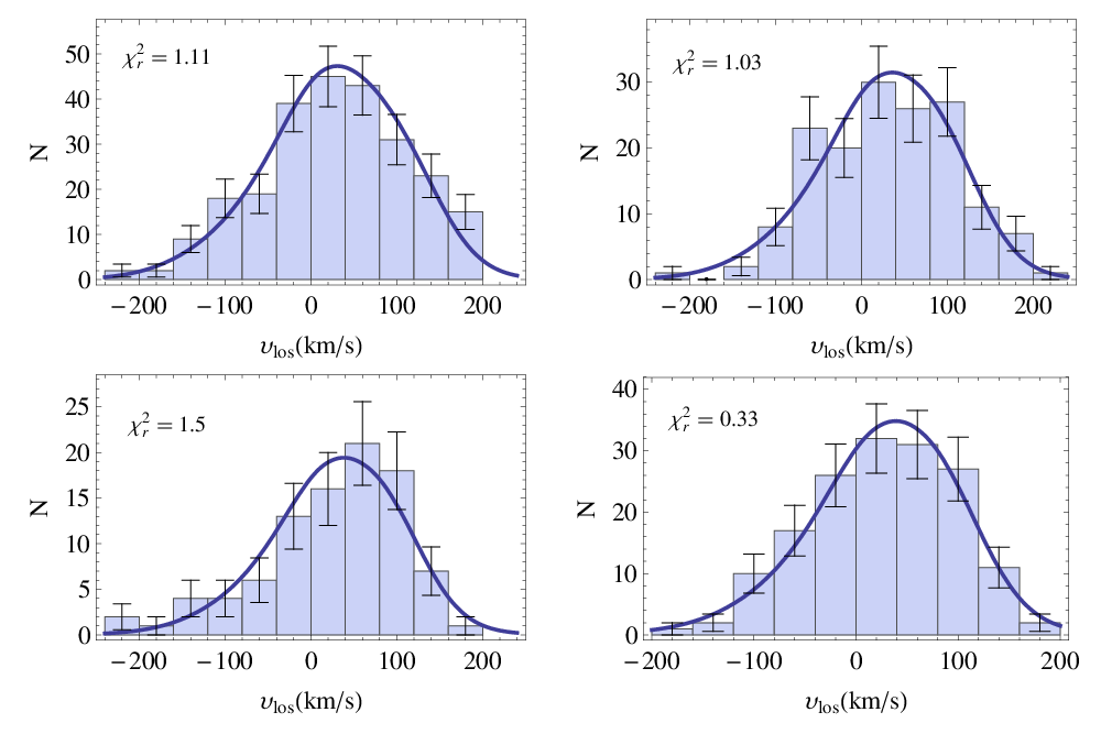
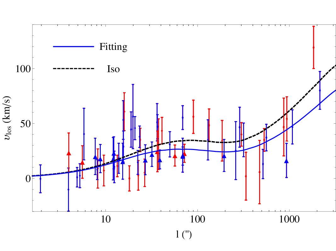
As in the spherical case, to model the rotation we add an odd part in to the initial even part of the distribution function, so that the final DF takes the form . We use again equation (17); this adds two additional parameters (, F) to the DF. Equation (19) gives the mean los velocity vs Galactic longitude. In order to constrain the parameters (, F) we fitted the mean los velocity from equation (19) to the los velocity data for all cells in Fig. 2. The best parameter values resulting from this 2D-fitting are , and . Figure 24 shows that the VPs of this rotating model compare well with the observed los VHs.
An axisymmetric system with a DF of the form is an isotropic rotator when all three eigenvalues of the dispersion tensor are equal (Binney & Tremaine, 2008) and therefore
| (56) |
In order to calculate from equation (56) it is not necessary for the DF to be known since and are already known from the Jeans equations (4.1). Figure 16 shows the fitted velocity from the DF against the isotropic rotator case calculated from equation (56), together with the mean los velocity data. The two curves agree well within , and also out to they differ only by km/s. Therefore according to our best model the NSC is close to an isotropic rotator, with slightly lower rotation and some tangential anisotropy outwards of 30”.
5 Discussion
In this work we presented a dynamical analysis of the Milky Way’s nuclear star cluster (NSC), based on 10’000 proper motions, 2’700 radial velocities, and new star counts from the companion paper of Fritz et al. (2014). We showed that an excellent representation of the kinematic data can be obtained by assuming a constant mass-to-light ratio for the cluster, and modeling its dynamics with axisymmetric two-integral distribution functions (2I-DFs), . The DF modeling allows us to see whether the model is physical, i.e., whether the DF is positive, and to model the proper motion (PM) and line-of-sight (los) velocity histograms (VHs). One open question until now has been the nature of the double peaked VHs of the -velocities along Galactic longitude, and the bell-shaped VHs of along Galactic latitude, which cannot be fitted by Gaussians (Schödel et al., 2009). Our 2I DF approximation of the NSC gives an excellent prediction for the observed shapes of the -, , and -VHs. The models show that the double-peaked shape of the -VHs is a result of the flattening of the NSC, and suggest that the cluster’s dynamical structure is close to an isotropic rotator. Because both PMs and los-velocities enter the dynamical models, we can use them also to constrain the distance to the GC, the mass of the NSC, and the mass of the Galactic centre black hole. To do this efficiently, we used the semi-isotropic Jeans equations corresponding to 2I-DFs. In this section, we discuss these issues in more detail.
5.1 The dynamical structure of the NSC
The star count map derived in Fritz et al. (2014) suggests two components in the NSC density profile, separated by an inflection point at about pc (see Fig. 7 above). To account for this we constructed a two-component dynamical model for the star counts in which the two components are described as independent -models. The inner, rounder component can be considered as the proper NSC, as in Fritz et al. (2014), while the outer, much more flattened component may represent the inner parts of the nuclear stellar disk (NSD) described in Launhardt et al. (2002).
The scale radius of the inner component is , close to the radius of influence of the SMBH, (Alexander, 2005). The profile flattens inside to a possible core (Buchholz et al., 2009; Fritz et al., 2014) but the slope of the three-dimensional density profile for the inner component is not well-constrained.
The flattening for the inner NSC component inferred from star counts is , very close to the value of found recently from Spitzer multi-band photometry (Schödel et al., 2014). It is important that these determinations agree with the dynamical flattening of our best Jeans dynamical models: the dynamical flattening is robust because it is largely determined by the ratio of and the tensor virial theorem. Because star counts, photometric, and dynamical values for the inner NSC flattening agree, this parameter can now be considered securely determined.
Assuming constant mass-to-light ratio for the NSC, we found that a 2I-DF model gives an excellent description of the proper motion and los velocity dispersions and VHs, in particular of the double-peaked distributions in the -velocities. This double-peaked structure is a direct consequence of the flattening of the star cluster; the detailed agreement of the model VPs with the observed histograms therefore confirms the value for the inner cluster component. For an axisymmetric model rotation cannot be seen directly in the proper motion VHs when observed edge-on, as is the case here, but is apparent only in the los velocities. When a suitable odd part of the DF is added to include rotation, the 2I-DF model also gives a very good representation of the skewed los VHs. From the amplitude of the required rotation we showed that the NSC can be approximately described as an isotropic rotator model, rotating slightly slower than that outside .
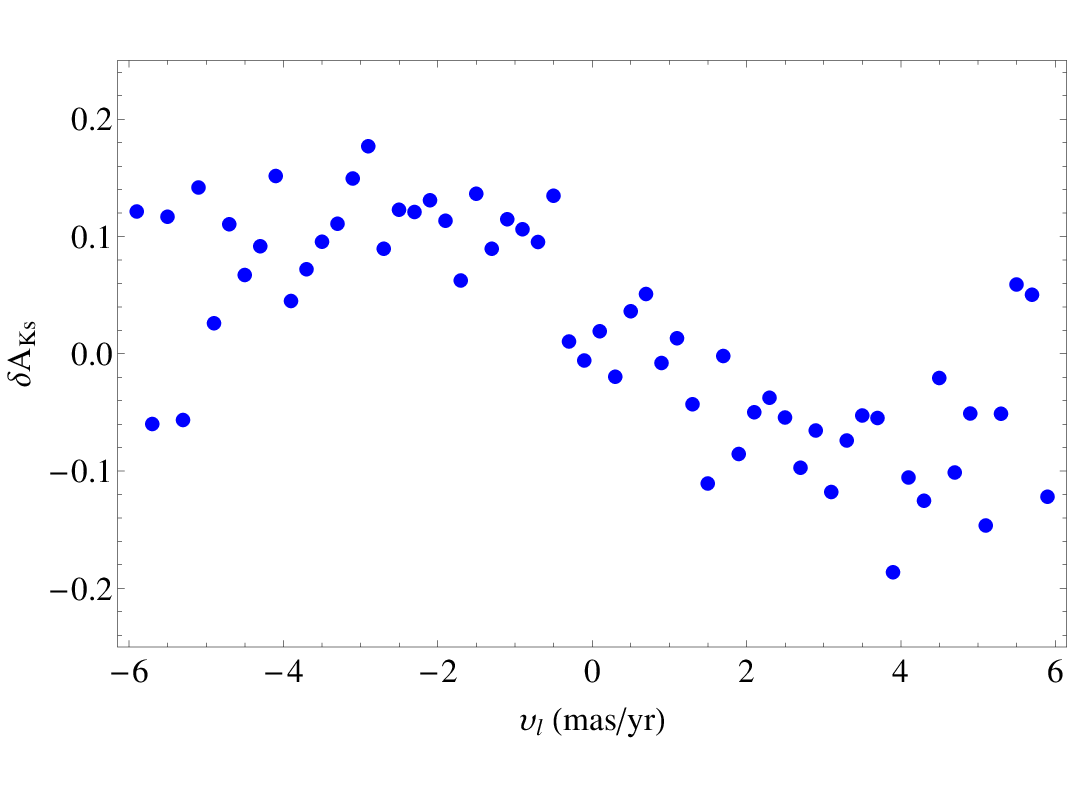
Individual VHs are generally fitted by this model within the statistical errors, but on closer examination the combined VHs show a slightly lower peak at negative velocities, as already apparent in the global histograms of Trippe et al. (2008); Schödel et al. (2009). Fig. 17 suggests that differential extinction of order mag within the cluster may be responsible for this small systematic effect, by causing some stars from the back of the cluster to fall out of the sample. The dependence of mean extinction on independently shows that the NSC must be rotating, which could otherwise only be inferred from the los velocities. In subsequent work, we will model the effect of extinction on the inferred dynamics of the NSC. This will then also allow us to estimate better how important deviations from the 2I-dynamical structure are, i.e., whether three-integral dynamical modeling (De Lorenzi et al., 2013, e.g.,) would be worthwhile.
5.2 Mass of the NSC
The dynamical model results in an estimate of the mass of the cluster from our dataset. Our fiducial mass value is interior to a spheroidal major axis distance . This corresponds to an enclosed mass within 3-dimensional radius of .
The fiducial mass for the best axisymmetric model is larger than that obtained with spherical models. The constant M/L spherical model with density parameters as in Section 3, for kpc and the same black hole mass has .
There are two reasons for this difference: (i) At where the model is well-fixed by kinematic data the black hole still contributes more than half of the interior mass. In this region, flattening the cluster at constant mass leaves and approximately constant, but decreases to adjust to the shape. To fit the same observed data, the NSC mass must be increased. (ii) Because of the increasing flattening with radius, the average density of the axisymmetric model decreases faster than that of the spherical density fit; thus for the same observed velocity dispersion profiles a larger binding mass for the NSC is required.
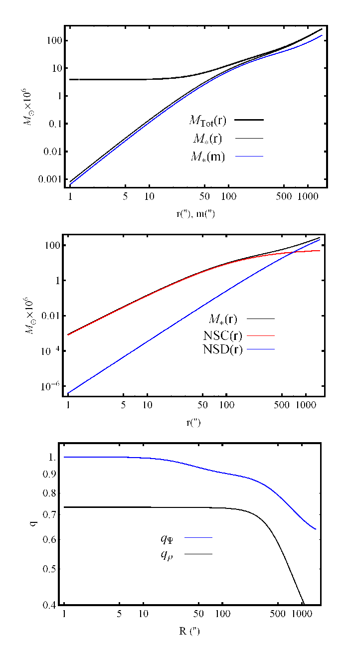
Figure 18 shows the enclosed stellar mass within the spheroidal radius as in equation (41), as well as the mass within the spherical radius . E.g., the mass within pc () is . This is compatible with the spherical modeling of Schödel et al. (2009) who gave a range of , rescaled to kpc, with the highest mass obtained for their isotropic, constant M/L model. According to Fig. 18, at pc the NSC contributes already of the interior mass ( at pc), and beyond pc it clearly dominates.
An important point to note is that the cluster mass does not depend on the net rotation of the cluster but only on its flattening. This is because to add rotation self-consistently to the model we need to add an odd part to the DF which does not affect the density or the proper motion dispersions and .
Our NSC mass model can be described as a superposition of a moderately flattened nuclear cluster embedded in a highly flattened nuclear disk. The cumulative mass distributions of the two components are shown in the middle panel of Figure 18. The NSD starts to dominate at about which is in good agreement with the value found by Launhardt et al. (2002).
Approximate local axis ratios for the combined density and for the total potential including the central black hole are shown in the lower panel of Fig. 18. Here we approximate the axial ratio of the density at radius by solving the equation for z and writing , and similarly for . The density axis ratio shows a strong decrease between the regions dominated by the inner and outer model components. The equipotentials are everywhere less flattened. At the center, because of the black hole; the minimum value is not yet reached at . Therefore, we can define the NSC proper as the inner component of this model, similar to Fritz et al. (2014).
The total mass of the inner component, (Section 4.2), is well-determined within similar relative errors as . However, identifying with the total mass of the Galactic NSC at the center of the nuclear disk has considerable uncertainties: because the outer NSD component dominates the surface density outside , the NSC density profile slope at large radii is uncertain, and therefore the part of the mass outside ( of the total) is also uncertain. A minimal estimate for the mass of the inner NSC component is its mass within up to where it dominates the star counts. This gives .
Finally, we use our inferred dynamical cluster mass to update the K-band mass-to-light ratio of the NSC. The best-determined mass is within . Comparing our with the K-band luminosity of the old stars derived in Fritz et al. (2014), , we obtain . The error is dominated by the uncertainty in the luminosity (21%, compared to a total 10% in mass from adding statistical and systematic errors in quadrature). The inferred range is consistent with values expected for mostly old, solar metallicity populations with normal IMF (Courteau et al., 2013; Fritz et al., 2014, e.g.,).
5.3 Evolution of the NSC
After half mass relaxation times a dense nuclear star cluster will eventually evolve to form a Bahcall-Wolf cusp with slope (Merritt, 2013); for rotating dense star clusters around black holes this was studied by Fiestas & Spurzem (2010). The minimum allowable inner slope for a spherical system with a black hole to have a positive DF is . From the data it appears that the Galactic NSC instead has a core (Buchholz et al., 2009; Fritz et al., 2014), with the number density possibly even decreasing very close to the center ( pc). This is far from the expected Bahcall-Wolf cusp, indicating that the NSC is not fully relaxed. It is consistent with the relaxation time of the NSC being of order Gyr everywhere in the cluster (Merritt, 2013).
From Fig. 16 we see that the rotational properties of the Milky Way’s NSC are close to those of an isotropic rotator. Fiestas et al. (2012) found that relaxation in rotating clusters causes a slow () evolution of the rotation profile. Kim et al. (2008) found that it also drives the velocity dispersions towards isotropy; in their initially already nearly isotropic models this happens in . On a similar time-scale the cluster becomes rounder (Einsel & Spurzem, 1999). Comparing with the NSC relaxation time suggests that these processes are too slow to greatly modify the dynamical structure of the NSC, and thus that its properties were probably largely set up at the time of its formation.
The rotation-supported structure of the NSC could be due to the rotation of the gas from which its stars formed, but it could also be explained if the NSC formed from merging of globular clusters. In the latter model, if the black hole is already present, the NSC density and rotation after completion of the merging phase reflects the distribution of disrupted material in the potential of the black-hole (Antonini et al., 2012, e.g.). Subsequently, relaxation would lead to shrinking of the core by a factor of in Gyr towards a value similar to that observed (Merritt, 2010). In the simulations of Antonini et al. (2012), the final relaxed model has an inner slope of , not far from our models (note that in flattened semi-isotropic models the minimum allowed slope for the density is also 0.5 (Qian et al., 1995)). Their cluster also evolved towards a more spherical shape, however, starting from a configuration with much less rotation and flattening than we inferred here for the present Milky Way NSC. Similar models with a net rotation in the initial distribution of globular clusters could lead to a final dynamical structure more similar to the Milky Way NSC.
5.4 Distance to the Galactic center
From our large proper motion and los velocity datasets, we obtained a new estimate for the statistical parallax distance to the NSC using axisymmetric Jeans modeling based on the cluster’s inferred dynamical structure. From matching our best dynamical model to the proper motion and los velocity dispersions within approximately , we found kpc. The statistical error is very small, reflecting the large number of fitted dispersion points. The systematic modeling error was estimated from uncertainties in the density structure of the NSC, as discussed in Section 4.2.
Our new distance determination is much more accurate than that of Do et al. (2013) based on anisotropic spherical Jeans models of the NSC, kpc, but is consistent within their large errors. We believe this is mostly due to the much larger radial range we modeled, which leaves less freedom in the dynamical structure of the model.
The new value for is in the range kpc found by Gillessen et al. (2009) from analyzing stellar orbits around Sgr A∗. A joint statistical analysis of the NSC data with the orbit results of Gillessen et al. (2009) gives a new best value and error kpc (Fig. 12, Section 4.2). Our estimated systematic error of kpc for in the NSC modeling translates to a similar additional uncertainty in this combined measurement.
Measurements of prior to 2010 were reviewed by Genzel et al. (2010). Their weighted average of direct measurements is kpc, where the first error is the variance of the weighted mean and the second the unbiased weighted sample variance. Two recent measurements give kpc from RR Lyrae stars (Dekany et al., 2013) and kpc from fitting axially symmetric disk models to trigonometric parallaxes of star forming regions (Reid et al., 2014). These measurements are consistent with each other and with our distance value from the statistical parallax of the NSC, with or without including the results from stellar orbits around Sgr A∗, and the total errors of all three measurements are similar, .
5.5 Mass of the Galactic supermassive black hole
Given a dynamical model, it is possible to constrain the mass of the central black hole from 3D stellar kinematics of the NSC alone. With axisymmetric Jeans modeling we found , where the systematic modeling error is estimated from the difference between models with different inner cluster flattening as discussed in Section 4.2. Within errors this result is in agreement with the black hole mass determined from stellar orbits around Sgr A∗ (Gillessen et al., 2009).
Our dataset for the NSC is the largest analyzed so far, and the axisymmetric dynamical model is the most accurate to date; it compares well with the various proper motion and line-of-sight velocity histograms. Nonetheless, future improvements may be possible if the uncertainties in the star density distribution and kinematics within 20” can be reduced, the effects of dust are incorporated, and possible deviations from the assumed 2I-axisymmetric dynamical structure are taken into account.
Several similar analyses have been previously made using spherical isotropic or anisotropic modeling. Trippe et al. (2008) used isotropic spherical Jeans modeling for proper motions and radial velocities in ; their best estimate is , much lower than the value found from stellar orbits. Schödel et al. (2009) constructed isotropic and anisotropic spherical broken power-law models, resulting in a black hole mass of . However, Fritz et al. (2014) find , also using a power-law tracer density. They argue that the main reason for the difference to Schödel et al. (2009) is because their velocity dispersion data for are more accurate, and their sample is better cleaned for young stars in the central . Assuming an isotropic spherical model with constant M/L, Fritz et al. (2014) find . Do et al. (2013) used 3D stellar kinematics within only the central pc of the NSC. Applying spherical Jeans modeling, they obtained which is consistent with that derived from stellar orbits inside , within the large errors. However, in their modeling they used a very small density slope for the NSC, of , which does not correspond to a positive DF for their quasi-isotropic model.
Based on this work and our own models in Section 4, the black hole mass inferred from NSC dynamics is larger for constant M/L models than for power law models, and it increases with the flattening of the cluster density distribution.
The conceptually best method to determine the black hole mass is from stellar orbits close to the black hole (Schödel et al., 2002; Ghez et al., 2008; Gillessen et al., 2009), as it requires only the assumption of Keplerian orbits and is therefore least susceptible to systematic errors. Gillessen et al. (2009) find that the largest uncertainty in the value obtained for is due to the uncertainty in , and that scales as . Therefore using our improved statistical parallax for the NSC also leads to a more accurate determination of the black hole mass. A joint statistical analysis of the axisymmetric NSC modeling together with the orbit modeling of Gillessen et al. (2009) gives a new best value and error for the black hole mass, (see Fig. 12, Section 4.2). An additional systematic error of 0.1 kpc for in the NSC modeling, through the BH mass-distance relation given in Gillessen et al (2009), translates to an additional uncertainty in .
Combining this result with the mass modeling of the NSC, we can give a revised value for the black hole influence radius , using a common definition of as the radius where the interior mass of the NSC equals twice the black hole mass (Merritt, 2013). Comparing the interior mass profile in Fig. 18 as determined by the dynamical measurement with , we obtain pc.
The Milky Way is one of some 10 galaxies for which both the masses of the black hole and of the NSC have been estimated (Kormendy & Ho, 2013). From these it is known that the ratio of both masses varies widely. Based on the results above we estimate the Milky Way mass ratio , with the error dominated by the uncertainty in the total NSC mass.
6 Conclusions
Our results can be summarized as follows:
- •
The density distribution of old stars in the central in the Galactic center can be well-approximated as the superposition of a spheroidal nuclear star cluster (NSC) with a scale length of and a much larger nuclear disk (NSD) component.
- •
The difference between the proper motion dispersions and cannot be explained by rotation alone, but is a consequence of the flattening of the NSC. The dynamically inferred axial ratio for the inner component is consistent with the axial ratio inferred from the star counts which for our two-component model is .
- •
The orbit structure of an axisymmetric two-integral DF gives an excellent match to the observed double-peak in the -proper motion velocity histograms, as well as to the shapes of the vertical -proper motion histograms. Our model also compares well with the symmetrized (even) line-of-sight velocity histograms.
- •
The rotation seen in the line-of-sight velocities can be modelled by adding an odd part of the DF, and this shows that the dynamical structure of the NSC is close to an isotropic rotator model.
- •
Fitting proper motions and line-of-sight dispersions to the model determines the NSC mass within , the mass of the SMBH, and the distance to the NSC. From the star cluster data alone, we find , , and kpc, where the estimated systematic errors account for additional uncertainties in the dynamical modeling. The fiducial mass of the NSC is larger than in previous spherical models. The total mass of the NSC is significantly more uncertain due to the surrounding nuclear disk; we estimate . The mass of the black hole determined with this approach is consistent with results from stellar orbits around Sgr A∗. The Galactic center distance agrees well with recent accurate determinations from RR Lyrae stars and masers in the Galactic disk, and has similarly small errors.
- •
Combining our modeling results with the stellar orbit analysis of Gillessen et al. (2009), we find and kpc. Because of the better constrained distance, the accuracy of the black hole mass is improved as well. Combining with the parameters of the cluster, the black hole radius of influence is pc () and the ratio of black hole to cluster mass is estimated to be .
References
- Aarseth et al. (1974) Aarseth S. J., Henon M., Wielen R. 1974 A&A 37,183
- Alexander (2005) Alexander T., 2005, Physics Reports, 419, 65
- Antonini et al. (2012) Antonini F., Capuzzo-Dolcetta R., Mastrobuono-Battisti A., Merritt D., 2012, ApJ, 750, 111
- Bahcall & Wolf (1976) Bahcall J. N., Wolf R. A., 1976, ApJ, 209, 214
- Böker et al. (2002) Böker T., Laine S., van der Marel R. P., et al., 2002, AJ, 123, 1389
- Böker et al. (2004) Böker T., Sarzi M., McLaughlin D. E., et al., 2004, AJ, 127, 105
- Böker (2010) Böker T., 2010, IAUS 266, 50
- Baes et al. (2005) Baes, M., Dejonge, H., & Buyle, P. 2005, A&A, 432, 411
- Binney & Tremaine (2008) Binney J. J., Tremaine S D., Galactic dynamics 2nd edition. Princeton University Press, Princeton
- Buchholz et al. (2009) Buchholz, R. M., Schodel, R., Eckart, A. 2009, A&A, 499, 483
- Bartko et al. (2010) Bartko H., et al. 2010, ApJ, 708, 834
- Chandrasekhar (1969) Chandrasekhar S. 1969, Ellipsoidal Figures of Equilibrium. Yale University Press, New Haven
- Carollo et al. (1997) Carollo C. M., Stiavelli M., de Zeeuw P. T., Mack J. 1997, AJ, 114, 2366
- Courteau et al. (2013) Courteau S., et al., 2013, RevModPhys, in press
- Deguchi et al. (2004) Deguchi S., Imai H., Fujii T., et al., 2004, PASJ, 56, 765
- Dehnen (1993) Dehnen W., 1993 MNRAS 269, 250
- Dehnen & Gerhard (1994) Dehnen W., Gerhard O. E., 1994, MNRAS, 268, 1019
- Dejonghe (1986) Dejonghe H. B. 1986, Phys. Re., 133, 218
- Dekany et al. (2013) Dekany I., Minniti D., Catelan M., Zoccali M., Saito R.K., Hempel M., Gonzalez O.A., 2013, ApJ, 776, L19
- De Lorenzi et al. (2013) De Lorenzi F., Hartmann M., Debattista V. P., Seth A. C., Gerhard O., 2013, MNRAS, 429, 2974
- Do et al. (2009) Do T., Ghez A. M., Morris M. R., Lu J. R., Matthews K., Yelda S., Larkin J., 2009, ApJ, 703, 1323
- Do et al. (2013) Do T., et al., 2013, ApJ, 779, L6
- Einsel & Spurzem (1999) Einsel, C., & Spurzem, R. 1999, MNRAS, 302, 81
- Ferrarese et al. (2006) Ferrarese L., Cˆot´e P., Jord´an A., et al., 2006, ApJS, 164,334
- Feldmeier et al. (2014) Feldmeier, A., Neumayer, N., Seth, A., Schödel, R., Lützgendorf, N., de Zeeuw, P. T., Kissler-Patig, M., Nishiyama, S., & Walcher, C. J. 2014, ArXiv e-prints
- Fiestas & Spurzem (2010) Fiestas, J., Spurzem, R., 2010, MNRAS, 405, 194
- Fiestas et al. (2012) Fiestas J., Porth, O., Berczik, P., Spurzem, R., MNRAS, 419, 57
- Fritz et al. (2011) Fritz T. K., et al. 2011, ApJ, 737, 73
- Fritz et al. (2014) Fritz T. K., Chatzpoulos S., Gerhard O., Gillessen S., Dodd-Eden K., Genzel R., Ott T. Pfuhl O., Eisenhauer F., 2014, submitted
- Genzel et al. (2010) Genzel R., Eisenhauer S., Gillessen S. 2010, Reviews of Modern Physics 82, 3121
- Genzel et al. (1996) Genzel, R., Thatte, N., Krabbe, A., Kroker, H., & Tacconi-Garman, L. E. 1996, ApJ, 472, 153
- Genzel et al. (2000) Genzel R., Pichon C., Eckart A., Gerhard O.E., Ott T., 2000, MRAS, 317, 348
- Ghez et al. (2008) Ghez A., et al., 2008, ApJ, 689, 104
- Graham & Spitler (2009) Graham A. W., Spitler L. R., 2009, MNRAS, 397, 2148
- Gillessen et al. (2009) Gillessen S., Eisenhauer S., Trippe S, Alexander T., Genzel R., Martins F., Ott T, 2009, ApJ, 707, L11
- Haller et al. (1996) Haller, J. W., Rieke, M. J., Rieke, G. H., et al. 1996, ApJ, 456, 194
- Hernquist (1990) Hernquist L., 1990, ApJ, 356,359
- Hunter & Qian (1993) Hunter C., Qian E., 1993, MNRAS, 202, 812
- Jaffe (1983) Jaffe W., 1983, MNRAS, 202, 995
- Kim et al. (2008) Kim E., Yoon I., Lee H.M., Spurzem R., 2008, MNRAS, 383, 2
- Kormendy & Ho (2013) Kormendy, J., Ho, L., 2013, ARAA, 51, 511
- Kuijken (1995) Kuijken K. 1995 MNRAS 446, 194
- Launhardt et al. (2002) Launhardt R., Zylka R., Mezger P.G., 2002, A&A, 384, 112
- Lindquist et al. (1992) Lindquist M., Winnberg A., Habing H.J., Matthews H.E., 1992, A&AS, 92, 43
- Lynden Bell (1960) Lynden-Bell D., 1960 MNRAS, 120, 204L
- Magorrian & Binney (1994) Magorrian J. Binney J., 1994 MNRAS, 271, 949
- Magorrian (1995) Magorrian J. 1995 MNRAS 277, 1185
- Merritt (2010) Merritt D., 2010, ApJ, 718, 739
- Merritt (2013) Merritt D., 2013. Dynamics and Evolution of Galactic Nuclei. Princeton, NJ: Princeton University Press
- Nagai & Miyamoto (1976) Nagai R., Miyamoto M., 1975, PASJ, 27, 533
- Qian et al. (1995) Qian E.E, de Zeeuw P.T., van der Marel R.P., Hunter C. 1995, MNRAS 274, 602
- Reid et al. (2014) Reid M.J., et al., 2014, arxiv:1401.5377
- Rossa et al. (2006) Rossa J., van der Marel R. P., B¨oker T., et al., 2006, AJ, 132, 1074
- Schödel et al. (2002) Schödel R., Ott T, Genzel R., et al., 2002, Nature, 419, 694
- Schödel et al. (2007) Schödel, R., et al., 2007, A&A, 469, 125
- Schödel et al. (2009) Schödel R., Merritt D., Eckart A.,2009, A&A, 502, 91
- Schödel et al. (2010) Schödel R., Najarro F., Muzic K., Eckart A., 2010, A&A, 511, A18
- Schödel et al. (2014) Schodel R., Feldmeier A., Kunneriath D., Stolovy S., Neumayer N., Amaro- ¨ Seoane P., Nishiyama S., 2014, preprint (arXiv:1403.6657)
- Seth et al. (2006) Seth A. C., Dalcanton J. J., Hodge P. W., Debattista V. P., 2006, AJ, 132, 2539
- Seth et al. (2008) Seth A., Agueros M., Lee D., Basu-Zych A., 2008, ApJ, 678, 116
- Tremaine et al. (1994) Tremaine S., Richstone, D. O., Byun, Y., Dressler, A., Faber, S. M., Grillmair, C., Kormendy, J., Lauer, T. R. 1994, AJ, 107, 634
- Trippe et al. (2008) Trippe S., et al., 2008, A&A 492, 419
- van de Ven et al. (2006) van de Ven G., van den Bosch R. C. E., Verolme E. K., de Zeeuw P. T., 2006, A&A, 445, 513
- Walcher et al. (2005) Walcher, C. J., van der Marel, R. P., McLaughlin, D., et al. 2005, ApJ, 618, 237
- Wehner & Harris (2006) Wehner E. H., Harris W. E., 2006, ApJL, 644, L17
- (66) Wolfram Research, Inc., Mathematica, Version 8.0, Champaign, IL (2011)
Appendix A Two-integral distributions functions
In this part we give implementation instructions for the 2I-DF algorithm of Hunter & Qian (1993, HQ). We will try to focus on the important parts of the algorithm and also on the tests that one has to make to ensure that the implementation works correctly. Our implementation is based on Qian et al. (1995) and made with Wolfram Mathematica (). For the theory the reader should consider the original HQ paper.
We will focus on the even part of the DF and for the case where the potential at infinity, , is finite and therefore can be set to zero. First one partitions the space where takes values in . The goal of the HQ algorithm is to calculate the value of the DF on each of these points on a 2D grid and subsequently end up with a 3D grid where we can apply an interpolation to obtain the final smooth function . The energy values on the 2D grid are placed logarithmically within an interval of interest (higher value is closer to the center) and the values of are placed linearly between 0 and 1. Physically allowable and correspond to bound orbits in the potential and therefore . In addition at each energy there is a maximum physically allowed corresponding to circular orbits with . This is given by the equations:
where is the radius of the circular orbit and the value is the maximum allowed value of at a specific . The function can be found by solving the 1st equation for and substituting in the second one therefore making a map . The value of the potential of a circular orbit with energy is denoted by and can be found from after solving the 1st of equation (A) for . The value is important for evaluation of and it is used in the contour of the complex integral.
To calculate the even part of the DF for each point of the grid we have to apply the following complex contour integral on the complex -plane using a suitable path:
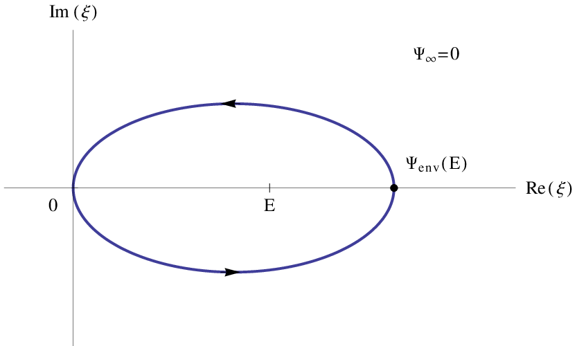
where the subscripts denotes the second partial derivative with respect to the first argument. A possible path for the contour is shown in figure A. The loop starts at the point 0 on the lower side of the real axis, crosses the real axis at the point and ends at the upper side of real axis. The parametrization of the path in general could be that of an ellipse:
| (61) |
where is the highest point of the ellipse. The value of should not be too high because we want to avoid other singularities but not too low either to maintain the accuracy. We optimize our implementation by integrating along the upper part of the loop and multiply the real part of the result by 2 (this is because of the Schwarz reflection principle).
In order to calculate the integrand of the integral we need the following transformation:
| (62) |
in which each subscript denotes a partial differentiation with respect to . This equation is analogous to equation (8) of the spherical case. In addition is the density considered as a function of and as opposed to and . The integrand of the contour integral A depends only on angle for a given pair. Therefore we need the maps and in order to find the value of the integrand for a specific . The first map is given by . The second is given by solving the equation for . It is very important that the solution of the previous equation corresponds to the correct branch in which the integrand attains its physically achieved values. In order to achieve that for each pair we start at the point which belongs to the physical domain and we look for the unique real positive solution. For the next point of the contour we use as initial guess the value of from the previous step that we already know that belongs to the correct branch. Using this method we can calculate the integrand in several values of then make an interpolation of the integrand and calculate the value of the DF using numerical integration.
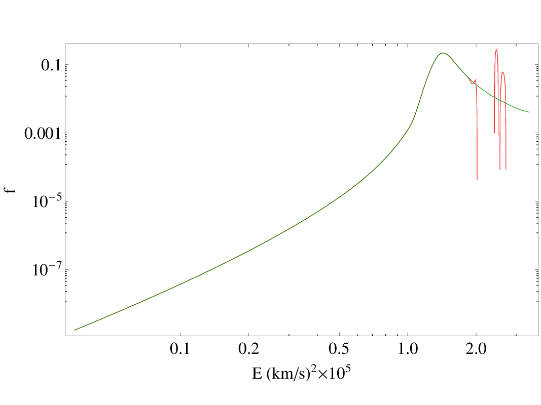
Figure 20 shows the shape of the DF for for the potential we use in the fourth section of the paper for one value of , using the aforementioned procedure. We notice that for large energies fluctuations of the DF appear. In order to solve this we introduce a minor improvement of the procedure, by generalizing the value of the contour to an energy-dependent function . The could be a simple step function that takes four or five different values. For our model the function is a decreasing function of . This means that the minor axis of the ellipse should decrease as the increases to avoid such fluctuations. In general we can write so that the contour depends both on and .
Once we implement the algorithm it is necessary to test it. Our first test is to check that the lower half of the integration path in figure A is the complex conjugate of the upper half. Probably the next most straightforward test is against the spherical case. It is possible to use the HQ algorithm to calculate a DF for spherical system. This DF should be equal to that obtained from Eddington’s formula for the same parameters. After calculating our 2I-DF we compare its low-order moments with those of Jeans modeling. The 0th and 2nd moments of the DF (the 1st is 0 for the even part) are given from the integrals.
Comparison with the 0th moment (density) is straight forward since the density is analytically known from the start. The 1st moments should be 0 within the expected error. In our implementation the error between Jeans modeling and the DF is of the order of within the area of interest. An additional test would be to integrate the VPs over the velocity space. Since the VPs integrals are normalized with the surface density the integral of a VP over the whole velocity space should be 1 within the expected error.
Appendix B VELOCITY HISTOGRAMS FOR THE 2-I MODEL