Flicker as a tool for characterizing planets through Asterodensity Profiling

In order to investigate whether a relation exists between flicker and mean stellar density, we first require an accurate catalog of stellar densities. Following B13, we identify the sample of Kepler targets for which asteroseismology oscillation modes have been detected as our “gold standard” catalog. These asteroseismology detections provide two immediate basic parameters: the average large frequency separation between consecutive overtones of the same spherical angular degree, $\Delta\nu$, and the frequency of maximum oscillations power, $\nu_{\mathrm{max}}$. This latter term has been shown to be functionally dependent, to a good approximation, upon the surface gravity of the host star, $g_{\star}$, and the effective temperature, $T_{\mathrm{eff}}$, [8, 22, 10, 6] via:

where $\nu_{\mathrm{max},\odot}$ is Sun’s frequency of maximum oscillations power, $T_{\mathrm{eff},\odot}$ is the Sun’s effective temperature and $g_{\odot}$ is the Sun’s surface gravity. The derived surface gravity is therefore moderately dependent upon some independent measure of the effective temperature. The other basic seismic observable, $\Delta\nu$, scales with the star’s mean stellar density [30] as:

where $\rho_{\odot}$ is the Sun’s mean density. In practice, this scaling is only approximate, and comparisons to individual model frequencies have shown temperature-dependent offsets of up to 2% in $\Delta\nu$ [32]. Nevertheless, $\rho_{\star}$ has a weaker functional dependence on the input effective temperature than $g_{\star}$ and detailed seismic modeling allows for a refined measurement of $\rho_{\star}$ at the percent level. For this reason, we consider that the seismic densities are the most accurate and precise parameter revealed by asteroseismology and so provide an ideal catalog for later calibration to flicker estimates.

In this work, we use the catalogs of Huber et al. [17] and Chaplin et al. [12], which include 588 distinct Kepler target stars. In the case of the catalog from Chaplin et al. [12], three different estimates of $\rho_{\star}$ are available, which vary very slightly due to different assumed effective temperatures and metallicities (Tables 4, 5 & 6). Of these, we preferentially employ Table 6 values wherever available (using high resolution spectroscopic stellar inputs from Bruntt et al. 9), then Table 5 values (IRFM $T_{\mathrm{eff}}$ and field-average metallicity values) and finally Table 4 in all other cases (using SDSS-calibrated $T_{\mathrm{eff}}$ and field-average metallicity values). In the few cases where both Huber et al. [17] and Chaplin et al. [12] have independent measures, we use Huber et al. [17] due to their use of dedicated spectroscopic inputs. In all cases, $\rho_{\star}$ uncertainties are also available, to provide the relevant weightings in the later regressions (see §II.3).

Following Basri et al. [4], and further described in B13, we measure the high-frequency stellar noise ($F_{8}$) in the standard pipeline processed PDC-MAP (data release 21) Kepler long-cadence (30 min) light curves by calculating the root-mean-square (RMS) of the difference between the light curve and a box-car smoothed version of itself. Basri et al. [4] originally defined the high-frequency noise using a 4-point smoothing, however B13 found that a 16-point (8-hr) smoothing yielded the cleanest correlation between the resultant $F_{8}$ and asteroseismically measured $\log g_{\star}$. Large excursions in the light curve, caused, for example, by stellar flares, can artificially inflate the measured $F_{8}$, resulting in erroneously low $F_{8}$-based $\log g_{\star}$. As such, we clip all $2.5$ $\sigma$ or greater outliers in the light curve prior to taking the RMS. For stars with known transiting exoplanets, such as those in Huber et al. [17], we additionally excise in-transit data points using the planetary orbital parameters publicly available through the NASA Exoplanet Archive [1]. We then correct this derived $F_{8}$ for shot noise contributions as described in B13. We compute $F_{8}$ for all available quarters of Kepler data and adopt our final estimate and associated uncertainty as the mean and standard deviation of the results, respectively.

We here describe how we compute the “best-fitting” model describing the dependent variable, $\rho_{\star}$, with respect to the independent variable, $F_{8}$. We begin by noting that the correlation between these terms is close to linear using log-log scaling (see Fig. 1), similar to the case when B13 compared $\log g_{\star}$ to $F_{8}$. Switching to log-log scaling requires an adjustment of the uncertainties in both variables. Uncertainties are known for both the $\rho_{\star}$ (see §II.1) and $F_{8}$ (see §II.2) measurements, which may be converted into $\log_{10}$ space using the general rule:

where $z$ is each variable and $\sigma_{z}$ is the associated uncertainty. Next, we consider that any model employed will itself be somewhat erroneous; i.e. there are not only uncertainties on the observables, but also in the model itself. For example, this could be because other terms not considered here also impact the observed flicker. We adopt a simple method to treat the model uncertainty by introducing a quadrature error term in the dependent variable, $\log_{10}\rho_{\star}$, given by $\sigma_{\mathrm{model}}$. This is similar to the way in which stellar “jitter” is often treated in radial velocity regressions [33] and implicitly assumes that the model error does not vary with respect to the independent variable.

Although the fractional uncertainties on the $\log_{10}F_{8}$ measurements are typically much greater than those of $\log_{10}\rho_{\star}$, we seek a regression technique which accounts for the appropriate weighting in both observables. Accordingly, our regression is performed in the least-squares framework, but specifically using the generalized Deming [15] method, which accounts for the uncertainties in both variables. We adopt a simple linear slope model given by Equation 4, motivated by the visual correlation (see Fig. 1) and the simplicity of this model makes it attractive for wider use in the community.

To perform a Deming regression, we must determine the co-ordinates of the point along the model curve, $y(x)$ (where $y$ and $x$ denote the dependent and independent variables respectively), which has the closest Euclidean distance to each trial point, $\{x_{i},y_{i}\}^{T}$. This is achieved by minimizing the metric $(x_{c,i}-x_{i})^{2}+(y(x_{c,i})-y_{i})^{2}$ with respect to $x_{c,i}$, where $\{x_{c,i},y_{c,i}\}^{T}$ is the point along the curve $y(x)$ closest to the trial point $\{x_{i},y_{i}\}^{T}$, which for our linear slope model gives:

The least-squares merit function, which we numerically minimize with respect to $\alpha$ and $\beta$, is simply the weighted Euclidean distance between the observations and the model:

where in our specific case we have $x_{i}\to\log_{10}\big(F_{8}\,[\mathrm{ppm}]\big)$, $y_{i}\to\log_{10}\big(\rho_{\star}\,[\mathrm{kg}\,\mathrm{m}^{-3}]\big)$, $\sigma_{x,i}^{2}\to\sigma_{\log_{10}(F_{8}\,[\mathrm{ppm}])}^{2}$ and $\sigma_{y,i}^{2}\to\sigma_{(\rho_{\star}\,[\mathrm{kg}\,\mathrm{m}^{-3}])}^{2}+\sigma_{\mathrm{model}}^{2}$.

If we assume that the residuals of the dependent variable to the best-fitting model are approximately normally distributed, then one would expect, for a well-chosen $\sigma_{\mathrm{model}}$, that the residuals divided by the respective uncertainties would be well described by the standard normal distribution. This can be checked by a subsequent least-squares regression of a normal distribution of zero mean but freely fitted variance to the distribution of the residuals. In practice, this is performed on the cumulative distribution of the residuals, rather than a probability density histogram, to avoid the choice of the bin-size affecting the results [20]. In general, an arbitrary guess of $\sigma_{\mathrm{model}}$ will lead to a non-unity variance for this regressed normal distribution, but we iterate $\sigma_{\mathrm{model}}$ until this condition is satisfied in order to solve for the best $\sigma_{\mathrm{model}}$.

Following the method described in §II.3, the best-fitting (mean maximum likelihood) model is shown in Fig. 1. Our simple linear model provides an excellent description of the apparent correlation and the associated parameters are available in Table 1. To compute this model, we enforced several criteria to exclude some of the less reliable data.

• $\blacksquare$

  $1.2<\log_{10}\big(F_{8}\,[\mathrm{ppm}]\big)\leq 2.2$ since we have relatively few points outside of this range.

• $\blacksquare$

  Range$\leq 1000$ ppm (defined in B13), since B13 find these points to be more frequently outliers.

• $\blacksquare$

  $4500\leq T_{\mathrm{eff}}<6500$ K to avoid the very cool or hot stars in our sample.

• $\blacksquare$

  $K_{P}<14$ since correcting $F_{8}$ for Kepler apparent magnitude is only calibrated up to this level (B13).

Note that the first criterion is equivalent to $3.25\lesssim\log g_{\star}\lesssim 4.43$ using the B13 relation, thus eliminating M & K dwarfs with insufficient photometric variability. These filters reduce the number of data points from 588 to 439. The 439 “good” points are denoted by circles in Fig. 1 and the ignored “bad” points are denoted by squares. Using only the good points, we find the model error is 0.14 dex (32% in $\rho_{\star}$). Including all the data increases this to 0.15 dex (35% in $\rho_{\star}$) and the fitted parameters are provided in Table 1.

Fig. 2 reveals that the residuals of the “good” sample appear approximately normally distributed. This means that if one knows the flicker of a star, one may construct an informative prior on $\log\rho_{\star}$ using a normal distribution and the parameters provided in Table 1. For the Sun’s observed flicker (B13), our relation yields $\rho_{\star}=(1.18\pm 0.37)$ $\rho_{\odot}$, compatible with the truth.

We repeated our regression on the “good” sample replacing $\log_{10}(\rho_{\star}\,[\mathrm{kg}\,\mathrm{m}^{-3}])$ with $\log_{10}(g_{\star}\,[\mathrm{cm}\,\mathrm{s}^{-2}])$. Since the dependent variables have been changed and use different units, a fair comparison of their relative performance cannot be conducted by inspection of the residuals in the dependent variables. Instead, we invert the best-fitting model to predict $F_{8}$ as a function of the dependent variable and then compute the residuals in the $F_{8}$ measurements between the two models.

We find that the $\rho_{\star}$ model has a standard deviation in $\log_{10}(F_{8}\,[\mathrm{ppm}])$ of $0.0866$ dex, versus $0.0824$ dex for the $\log g_{\star}$ model. We also note that the Pearson’s correlation coefficient is $-0.927$ for the $\rho_{\star}$ model but $-0.934$ for the $\log g_{\star}$ model. We therefore conclude that surface gravity is a slightly better dependent variable to correlate against $F_{8}$, although clearly $\rho_{\star}$ does an excellent job too (see Fig. 1). This weakly supports the hypothesis that flicker is most directly tracing surface features such as granulation [13], rather than internal processes. Further support of this is found when we compare $M_{\star}/R_{\star}$ to $F_{8}$, causing the correlation coefficient to drop to $-0.928$. The $\rho_{\star}$ relation is likely a good match simply due to the expected evolutionary correlation between $M_{\star}/R_{\star}^{2}$ and $M_{\star}/R_{\star}^{3}$. Nevertheless, the $\rho_{\star}$ relation is more useful when analyzing exoplanet transits, since this term directly affects the light curve shape [27].

Asterodensity profiling (AP) has recently emerged as a valuable tool for characterizing exoplanets using time series photometry [19, 29, 21]. AP exploits the fact that for a planet on a Keplerian circular orbit transiting an unblended star with a symmetric intensity profile, the shape of the light curve reveals $\rho_{\star,\mathrm{obs}}$ [27]. If any of the idealized assumptions are invalid, then $\rho_{\star,\mathrm{obs}}$ will differ from the true value, $\rho_{\star,\mathrm{true}}$, and the direction and magnitude of the discrepancy reveals information about the transiting system [21]. Using independent $\rho_{\star}$ estimates from asteroseismology, Sliski & Kipping [29] provide an example of the utility of AP by showing that the false positive rate of transiting planet candidates associated with giant stars is much higher than that of dwarf stars.

In this work, we have shown that flicker may also be used as an input for the independent measure of $\rho_{\star,\mathrm{true}}$ required for AP. Despite uncertainties in $\rho_{\star}$ increasing to $\sim 30$% from a flicker-based determination versus $\sim 4$% using asteroseismology, flicker can be used on many more targets in a magnitude-limited photometric survey like Kepler, since it works reliably down to $K_{P}=14$ (see later discussion in §IV.2). We do not claim that the derived relation is the optimal choice of regressors or parametric form, merely that it provides a simple, empirical recipe for estimating $\rho_{\star}$. For example, including effective temperature may improve the relation, since cooler stars seem to be found at higher flicker values (see Fig. 1). However, including such terms would make our relation no longer purely photometric, which we would argue is the principal benefit of the flicker technique.

Whilst we direct those interested to Kipping [21] for details on the theory and range of effects which can cause AP discrepancies, we here provide an example calculation of the sensitivity of AP using flicker to detect eccentric exoplanets via the so-called “photo-eccentric” effect [14]. For a planet on an eccentric orbit, the derived light curve stellar density will differ from the true value by [18]:

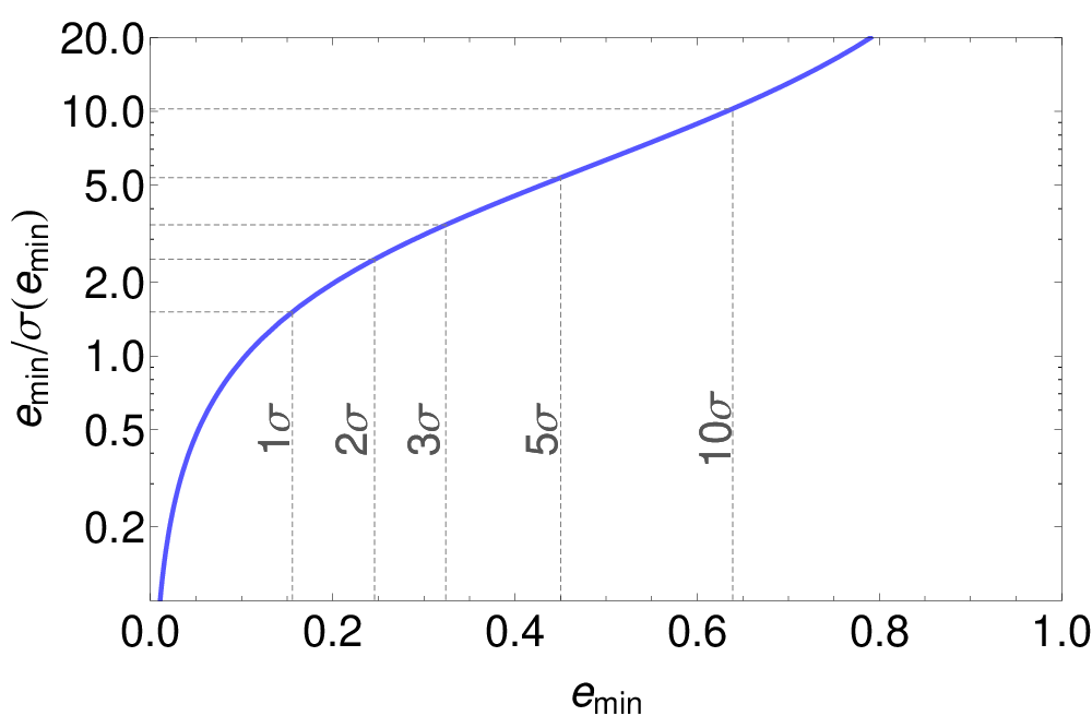
where $e$ is the orbital eccentricity and $\omega$ is argument of periastron. Dawson & Johnson [14] show how to first order, constraints on $e$ scale with $\rho_{\star,\mathrm{true}}^{1/3}$ and thus even a weak prior on the density can lead to useful constraints on $e$. With one observable and two unknowns, a unique solution to Equation 8 is not possible. However, one can derive the minimum eccentricity, $e_{\mathrm{min}}$, of the planet and the associated uncertainty, $\sigma_{e_{\mathrm{min}}}$, using Equations 39&40 of Kipping [21] respectively. Let us assume that the uncertainty in $(\rho_{\star,\mathrm{obs}}/\rho_{\star,\mathrm{true}})$ is dominated by the denominator’s error, which in turn was found using our flicker relation and equals 31.7%. We may now plot the term $(e_{\mathrm{min}}/\sigma_{e_{\mathrm{min}}})$ as a function of $e_{\mathrm{min}}$ in Fig. 3, to illustrate the ability of flicker to detect eccentric planets. Using the classic Lucy & Sweeney [23] test, we mark several key confidence levels with grid lines, demonstrating that flicker can detect eccentricities of $e_{\mathrm{min}}=0.25$ to $\geq 2$ $\sigma$ confidence and $e_{\mathrm{min}}=0.32$ to $\geq 3$ $\sigma$. With the power of large number statistics, we anticipate that flicker will be particularly powerful for inferring the ensemble distribution of orbital eccentricities.

Between the two catalogs of Huber et al. [17] and Chaplin et al. [12], there are 588 unique targets with asteroseismology detections yielding $\rho_{\star}$ measurements with a median uncertainty of 4.1%. In contrast, there are $28,577$ Kepler targets with $K_{P}<14$, $4500<T_{\mathrm{eff}}<6500$ K and $3.25<\log g<4.43$ (NASA Exoplanet Archive). Making the simple assumption that the same fraction of these targets will satisfy the range criterion defined earlier in §III.1, then we expect $\sim 25,000$ targets to be amenable for a flicker-based estimate of $\rho_{\star}$ with a model accuracy of 31.7%. This translates to an increase in the number of AP targets by a factor of $\sim 40$ at the expense of an increase in the measurement uncertainty by a factor of $\sim 8$. By any accounts, this is an acceptable compromise and opens the door to conducting AP on hundreds of Kepler planetary candidates (we estimate $\sim 630$).

An alternative method to determine $\rho_{\star,\mathrm{true}}$ for targets without detectable oscillations would be via spectroscopy (e.g. Dawson & Johnson 14). Here, one observes a spectrum of the target, compares it to a catalog of library spectra with various $T_{\mathrm{eff}}$, $[\mathrm{M}/\mathrm{H}]$ and $\log g_{\star}$ and then finally one finds the best matching stellar evolution isochrones to these basic parameters. This procedure has several drawbacks compared to a flicker-based determination though. Firstly, this method requires that one obtain high SNR spectra, whereas F8 can be measured from the data obtained directly from a photometric mission like Kepler. Secondly, the final determination of $\rho_{\star}$ is strongly model dependent using both stellar evolution models and spectra template matching laden with challenging degeneracies. Finally, it is worth noting that the formal uncertainty on a spectroscopic determination of $\rho_{\star,\mathrm{true}}$ is typically no better than the flicker-based empirical relation for Sun-like stars. For example, Dawson & Johnson [14] report $\rho_{\star,\mathrm{true}}=1.02_{-0.29}^{+0.45}$ $\rho_{\odot}$ for the $K_{P}=13.6$ Sun-like target KOI-686 and our flicker technique yields $(0.97\pm 0.44)$ $\rho_{\odot}$. In general then, we argue that for determinations of $\rho_{\star}$, the empirical and largely model independent flicker technique is preferable to spectroscopy, provided the target satisifies our sample criteria.

For the future TESS mission [26], the smaller lens aperture of 12 cm will lead to higher photon noise than Kepler, for the same target. We therefore expect the 14^th magnitude cut-off of our flicker calibration to drop to $\sim 11.5$. The same effect will lead to only very bright stars having asteroseismology detections though, with preliminary estimates suggesting $\sim 5\times 10^{3}$ asteroseismology targets out of $\sim 5\times 10^{5}$ target stars. In contrast, we expect that $\sim 10^{5}$ TESS targets will be amenable to a flicker-based determination of their stellar densities (with the exact number depending upon the as yet unknown target list). Similarly, we expect flicker to have majorly benefit the upcoming PLATO 2.0 mission [25] for both moderately bright targets near the edge of the field and faint targets in the center. Since AP is not only a method for characterizing exoplanets but also for vetting them [29], then we expect flicker to be an invaluable tool in the TESS and PLATO era.

References

- [1] Akeson, R. L. et al., 2013, PASP, 125, 989
- [2] Baglin, A., Michel, E., Auvergne, M. & COROT Team, 2006, in Proc. of the CoRoT Mission Pre-Launch Status—Stellar Seismology and Planet Finding, ed. M. Fridlund, A. Baglin, J. Lochard & L. Conroy (ESA SP-1306; Noordwijk: ESA), 39
- [3] Barnes, S. A., 2007, ApJ, 669, 1167
- [4] Basri, G. et al., 2011, AJ, 141, 20
- [5] Bastien, F. A., Stassun, K. G., Basri, G. & Pepper, J., 2013, Nature, 500, 427 (B13)
- [6] Belkacem, K. et al., 2011, A&A, 530, 142
- [7] Borucki, W. et al., 2008, in Pont F., Sasselov, D., Holman M. J., eds, Proc. IAU Symp. 253: Transiting Planets, p. 289
- [8] Brown, T. M., Gilliland, R. L., Noyes, R. W. & Ramsey, L. W., 1991, ApJ, 368, 599
- [9] Bruntt, H. et al., 2012, MNRAS, 423, 122
- [10] Chaplin, W. J., Houdek, G., Appourchaux, T., Elsworth, Y., New, R. & Toutain, T., 2008, A&A, 485, 813
- [11] Chaplin, W. J. & Miglio, A., 2013, ARA&A, 51, 353
- [12] Chaplin, W. J. et al., 2014, ApJS, 210, 1
- [13] Cranmer, S. R., Bastien, F. A., Stassun, K. G. & Saar, S. H., 2014, ApJ, 781, 124
- [14] Dawson, R. I. & Johnson, J. A., 2012, ApJ, 756, 13
- [15] Deming, W. E., 1943, Statistical Adjustment of Data, Wiley, New York, NY
- [16] Epstein, C. R. & Pinsonneault, M. H., 2014, ApJ, 780, 159
- [17] Huber, D. et al., 2013, ApJ, 767, 127
- [18] Kipping, D. M., 2010, MNRAS, 407, 301
- [19] Kipping, D. M., Dunn, W. R., Jasinksi, J. M. & Manthri, V. M., 2012, MNRAS, 421, 1166
- [20] Kipping, D. M., 2013, MNRAS, 434, L51
- [21] Kipping, D. M., 2014, MNRAS, accepted (astro-ph:1311.1170)
- [22] Kjeldsen, H. & Bedding, T. R., 1995, A&A, 293, 87
- [23] Lucy, L. B. & Sweeney, M. A., 1971, AJ, 76, 544
- [24] Mathur, S. et al., 2011, ApJ, 741, 119
- [25] Rauer, H et al., 2013, Exp. Astron., submmited (astro-ph:1310.0696)
- [26] Ricker, G. R. et al., 2010, in American astronomical society meeting abstracts #215, vol. 42 of Bulletin of the American Astronomical Society, p. 450.06
- [27] Seager, S. & Mallen-Ornélas, G., 2003, ApJ, 585, 1083
- [28] Skumanich, A., 1972, ApJ, 171, 565
- [29] Sliski, D. H. & Kipping, D. M., 2014, ApJ, submitted (astro-ph:1401.1207)
- [30] Ulrich, R. K., 1986, ApJ, 306, L37
- [31] Walkowicz, L. M. & Basri, G. S., 2013, MNRAS, 436, 1883
- [32] White, T. R., Bedding, T. R., Stello, D., Christensen-Dalsgaard, J., Huber, D. & Kjeldsen, H., 2011, ApJ, 743, 161
- [33] Wright, J. T., 2005, PASP, 117, 657