Contact Symplectic Fibrations and
Fiber Connected SumThanks: The author is partially supported by TUBITAK grant 1109B321200181 and also by NSF FRG grant DMS-1065910

Let $(B^{2n+1},\mu)$ be any contact manifold, and $(F^{2m},\beta)$ an exact symplectic manifold. Consider the product $B\times F$ and the standard projections given by

Consider the pull-back forms $\tilde{\mu}:=\pi_{1}^{\ast}(\mu)$, $\tilde{\beta}:=\pi_{2}^{\ast}(\beta)$ and set

Then by the binomial expansion formula and using the facts $(d\tilde{\mu})^{i}=0,\;\forall i\geq n+1$ and $(d\tilde{\beta})^{j}=0,\;\forall j\geq m+1$, we compute

Therefore, $\sigma\wedge(d\sigma)^{n+m}$ is a volume form on the product manifold $B\times F$ because $\mu\wedge(d\mu)^{n}$ and $(d\beta)^{m}$ are volume forms on $B$ and $F$, respectively. Hence, $\sigma$ is a contact form on $B\times F$. ∎

Let $(F\hookrightarrow E\stackrel{{\scriptstyle\pi}}{{\twoheadrightarrow}}B)_{G}$ be any given contact symplectic fibration with $\textrm{dim}(F)=2m$ and $\textrm{dim}(B)=2n+1$. By the fiber bundle structure, we know that up to diffeomorphism the total space $E$ is obtained by patching the trivial $F$-bundles, and the transition maps are contained in the structure group $G\subset\textrm{Exact}(F,\beta)$ where $(F,\beta)$ is any fixed fiber of $\pi$. More precisely, there is an open cover $\{U_{\alpha}\}_{\alpha}$ of $B$ and a collection of diffeomorphisms $\phi_{\alpha}:\pi^{-1}(U_{\alpha})\to U_{\alpha}\times F$ such that the diagram

commutes. Moreover, by restricting $\phi_{\alpha}$ to any fiber $F_{b}=\pi^{-1}(b)$ and then projecting onto $F$-factor, we get a smooth map $\phi_{\alpha}(b):F_{b}\to F$, and the transition maps $\phi_{\gamma\alpha}:U_{\alpha}\cap U_{\gamma}\to G\subset\textrm{Exact}(F,\beta)$ given by

Using paracompactness, one can find another open cover $\{V_{\rho}\}_{\rho}$ of $B$ such that for any index $\rho$ the closure $\overline{V}_{\rho}$ is contained in $U_{\alpha}$ for some $\alpha$. Since $B$ is compact (by assumption), there is a finite subcover $\{V_{1},V_{2},...,V_{r}\}$ of $\{V_{\rho}\}_{\rho}$. Here one can assume that $V_{i}$’s are listed in a specific order so that $V_{i}\cap V_{i+1}\neq\emptyset$ whenever $V_{i}$ and $V_{i+1}$ belong to the same connected component of $B$. Indeed, the argument below can be done independently for each connected component. Therefore, without loss of generality $B$ will be assumed to be connected. Now consider the collection $\mathcal{W}:=\{W^{i}\subset B\,|\,i=1,...,r\}$ of compact sets defined by

Clearly, $\mathcal{W}$ forms a partition for the base space $B$, that is, we have

for any $i,j$, $\textrm{int}(W^{i})\cap\textrm{int}(W^{j})=\emptyset$, and each union $W^{1}\cup W^{2}\cup\cdots\cup W^{i}$ intersects with $W^{i+1}$ along a smooth compact hypersurface

Observe that for each $i=1,...,r-1$ we have the map $\phi_{i}:H_{i}\to G\subset\textrm{Exact}(F,\beta)$ obtained by restricting the corresponding $\phi_{\gamma\alpha}$. More precisely, from the construction of $\{V_{\rho}\}_{\rho}$, we know for each $i$ and $j$ with $1\leq j\leq i$ that $W^{j}\subset U_{\alpha_{j}}$ and $W^{i+1}\subset U_{\gamma}$ for some $\alpha_{j},\gamma$. So one can define the map $\phi_{i}$ by patching the restrictions of $\phi_{\gamma\alpha_{j}}$ to the subsets $W^{j}\cap W^{i+1}\subset U_{\alpha_{j}}\cap U_{\gamma}$ together. As a result, up to diffeomorphism we obtain the description given by

where each $\Phi^{i}:H_{i}\times F\to H_{i}\times F$ is the smooth gluing map defined by

For each $i$ the fact that $\phi_{i}\in\textrm{Exact}(F,\beta)$ implies that there exists a smooth function $\psi_{i}:F\to\mathbb{R}$ such that $\phi_{i}^{*}(\beta)=\beta+d\psi_{i}$. In accordance with the smooth gluing map (or rule) $\Phi^{i}$, one can patch all these functions together which yields a smooth function $\Psi_{i}:H_{i}\times F\to\mathbb{R}$.

Next, in order to construct a compatible contact structure on $E$, we will use the above description as follows: By assumption $B$ admits a contact structure, say $\mu$. For any real number $K>0$, the $1$-form $K\mu$ is contact (indeed, the manifolds $(B,\textrm{Ker}(\mu))$ and $(B,\textrm{Ker}(K\mu))$ are contactomorphic, and their contact hyperplane distributions coincide everywhere on $B$). Also from Lemma 2.7 we know that for any $K>0$ the $1$-form $K\mu+\beta$ is a contact form on $B\times F$, and so, in particular, on each $W^{i}\times F$. (For simplicity, we will denote the pull-back of $\mu$ (resp. $\beta$) on any product space still by $\mu$ (resp. by $\beta$).

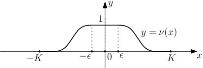
For a sufficiently small $\epsilon>0$ consider the tubular neighborhood $H_{1}\times[-\epsilon,\epsilon]$ of $H_{1}=W^{1}\cap W^{2}$ in $W^{1}\cup W^{2}$, and let $f_{1}:H_{1}\times[-\epsilon,\epsilon]\times F\longrightarrow\mathbb{R}$ be a smooth cut-off function defined by $f_{1}(b,x,p)=f(x)$ where $f:[-\epsilon,\epsilon]\to\mathbb{R}$ is the smooth cut-off function such that $f(x)\equiv 1$ on $(-\delta,\delta)$ for some $0<\delta<\epsilon$ and $f(x)\equiv 0$ for all $x$ near $\pm\epsilon$ as in Figure 1.

For a real number $K_{1}>0$, consider the smooth $1$-form $\sigma_{1}:=K_{1}\mu+\beta+f_{1}d\Psi_{1}$ on $H_{1}\times[-\epsilon,\epsilon]\times F$. By construction we can smoothly glue this form with the contact form $K_{1}\mu+\beta$ on $[(W^{1}\cup W^{2})-(H_{1}\times(-\epsilon,\epsilon)]\times F$. Also observe that $\sigma_{1}$ is in accordance with the gluing map $\Phi^{1}$ because for any fiber $F$ over the gluing region $H_{1}$ (where $f_{1}\equiv 1$) we have $\sigma_{1}|_{F}=\beta+d\psi_{1}=\phi_{1}^{*}(\beta)=(\Phi^{1}|_{F})^{*}(\beta)$. Therefore, $\sigma_{1}$ is, indeed, a smooth $1$-form on $(W^{1}\times F)\cup_{\Phi^{1}}(W^{2}\times F)$. Moreover, on the region $H_{1}\times[-\epsilon,\epsilon]\times F$ we compute

where $C_{1},C_{2},C_{3},C_{4}$ are constants detemined by the binomial expansion formula for $(d\sigma_{1})^{n+m}$, and we use the facts $(d\mu)^{i}=0,\;\forall i\geq n+1$ and $(d\beta)^{j}=0,\;\forall j\geq m+1$. Observe that if $K_{1}$ is chosen large enough, the first term on the right hand side is dominant over all other terms since it has the highest degree of $K_{1}$. Therefore, for $K_{1}$ large enough $\sigma_{1}\wedge(d\sigma_{1})^{n+m}$ is a volume form on $H_{1}\times[-\epsilon,\epsilon]\times F$, and hence $\sigma_{1}$ is a contact form on $(W^{1}\times F)\cup_{\Phi^{1}}(W^{2}\times F)$.

Now we want to extend $\sigma_{1}$ to a contact form on $(W^{1}\times F)\cup_{\Phi^{1}}(W^{2}\times F)\cup_{\Phi^{2}}(W^{3}\times F)$: For $\epsilon>0$ sufficiently small, consider the tubular neighborhood $H_{2}\times[-\epsilon,\epsilon]$ of $H_{2}=(W^{1}\cup W^{2})\cap W^{3}$ in $W^{1}\cup W^{2}\cup W^{3}$ such that $H_{2}\times[-\epsilon,0]\subset W^{3}$ and $H_{2}\times[0,\epsilon]\subset W^{1}\cup W^{2}$. Take a smooth cut-off function $g_{2}:H_{2}\times[-\epsilon,\epsilon]\times F\longrightarrow\mathbb{R}$ defined by $g_{2}(b,x,p)=g(x)$ where $g:[-\epsilon,\epsilon]\to\mathbb{R}$ is the smooth cut-off function such that $g(x)\equiv 1$ on $(-\delta,\epsilon]$ for some $0<\delta<\epsilon$ and $g(x)\equiv 0$ for all $x$ near $-\epsilon$ as in Figure 2.

For a real number $K_{2}>0$, we define the smooth $1$-form $\sigma_{2}:=K_{2}\mu+\beta+f_{2}d\Psi_{2}$ on $H_{2}\times[-\epsilon,\epsilon]\times F$ where $f_{2}=g_{2}f_{1}$. On the region $H_{2}\times[-\epsilon,\epsilon]\times F$, similar to the computation given in Equation (4) we have

which implies that if $K_{2}$ is chosen large enough, then $\sigma_{2}$ is contact on $H_{2}\times[-\epsilon,\epsilon]\times F$. Moreover, the functions $\Psi_{1}$ and $\Psi_{2}$ are identical on their overlaping domains because $\phi_{1}$ and $\phi_{2}$ are constructed using the same transition functions on their common domains. As a result, if we choose $K_{1}=K_{2}=\textrm{Max}(K_{1},K_{2})$, then by gluing with $\sigma_{1}$ we obtain a smooth contact form $\sigma_{2}$ on $(W^{1}\times F)\cup_{\Phi^{1}}(W^{2}\times F)\cup_{\Phi^{2}}(W^{3}\times F)$.

Next, we can repeatedly follow exactly the same lines of the last extension argument for the remaining parts of the description of $E$ given in Equation (3), and eventually obtain a contact form on $E$.

More precisely, for each $i=3,4,...,r-1$ and $\epsilon>0$ small enough, consider the smooth cut-off function $g_{i}:H_{i}\times[-\epsilon,\epsilon]\times F\longrightarrow\mathbb{R}$ defined by $g_{i}(b,x,p)=g(x)$. Here, similar to above, we assume that $H_{i}\times[-\epsilon,0]\subset W^{i+1}$ and $H_{i}\times[0,\epsilon]\subset W^{1}\cup\cdots\cup W^{i}$. Suppose that the contact form

is already constructed on the union $(W^{1}\times F)\cup_{\Phi^{1}}\cdots\cup_{\Phi^{i-1}}(W^{i}\times F)$, and it extends $\sigma_{i-2}$. Note that one needs to choose the constants $K_{j}$ ($j=1,2,...,i-1$) to be $K_{1}=K_{2}=\cdots=K_{i-1}=\textrm{Max}(K_{1},K_{2},...,K_{i-1})$ to perform this extension. Then one can similarly check as in Equation (5) that the form

is contact on $H_{i}\times[-\epsilon,\epsilon]\times F$ if $K_{i}$ is large enough. Moreover, one can see $\sigma_{i}$ as the extension of $\sigma_{i-1}$ to the union $(W^{1}\times F)\cup_{\Phi^{1}}\cdots\cup_{\Phi^{i}}(W^{i+1}\times F)$ once we do the reassignments

Finally, we set $\sigma:=\sigma_{r-1}$. Then by the construction $\sigma$ restricts to an exact symplectic structure on each fiber of $\pi$. So the contact form $\sigma$ defines a contact structure $\textrm{Ker}(\sigma)$ on $E$ which is compatible with the fibration map $\pi:E\to B$.

In order to prove the second statement, observe that if $G\subset\textrm{Exact}(F,\partial F,\beta)$, then for any transition map $\phi_{\alpha\gamma}$ used in the above construction and for any $b\in U_{\alpha}\cap U_{\gamma}$ we have $\phi_{\alpha\gamma}(b)\equiv Id_{F}$ near $\partial F$ (in particular, $\partial_{h}E\approx B\times\partial F$). Therefore, the smooth maps $\psi_{i}:F\to\mathbb{R}$ in the construction are all constant functions near $\partial F$, and so the corresponding functions $\Psi_{i}:H_{i}\times F\to\mathbb{R}$ take constant values near $\partial_{h}E$ (i.e., $d\Psi_{i}=0$ near $\partial_{h}E$). As a result, the description of the contact form $\sigma(=\sigma_{r-1})$ on $E$ given above takes the form $\sigma=K_{r-1}\mu+\beta$ near $\partial_{h}E$. ∎

Since $\eta_{0},\eta_{1}$ are isotopic, there exists a smooth family $\{\eta_{t}\,|\,t\in[0,1]\}$ of contact structures on $B$ joining them. Consider a smooth family $\{\alpha_{t}\,|\,t\in[0,1]\}$ of contact forms on $B$ such that $\alpha_{0}=\mu_{0}$ and $\textrm{Ker}(\alpha_{t})=\eta_{t}$ for all $t$. Since $\textrm{Ker}(\alpha_{1})=\eta_{1}=\textrm{Ker}(\mu_{1})$, we have $\alpha_{1}=h\mu_{1}$ for some smooth function $h:B\to\mathbb{R}^{+}$. Then we obtain the (modified) smooth family

of contact forms on $B$ joining $\mu_{0}$ and $\mu_{1}$ and with the property $\textrm{Ker}(\mu_{t})=\eta_{t}$ for all $t$.

Consider the bundle contact structure $\xi(\mu_{t})$ on $E$ associated to $\mu_{t}$ given by the contact form $\sigma_{t}=K^{t}_{r-1}\mu_{t}+\beta+f_{r-1}d\Psi_{r-1}$ constructed as in the proof of Theorem 2.3. In order to simplify the notation, we will write $K_{t}$ for $K^{t}_{r-1}$. Let us consider

$\mathcal{K}:=\{K_{t}\,|\,t\in[0,1]\}$.

For each $t$ the choice of $K_{t}$ can be done in such a way that $K_{t}$’s varies continuously with respect to $t$. This is possible since $\{\mu_{t}\,|\,t\in[0,1]\}$ is a smooth $1$-parameter family. Therefore, the set $\mathcal{K}$ can be realized as the range set of a continuous function on the compact set $[0,1]$, and hence there exists an upper bound, say $K_{upp}$, for $\mathcal{K}$. We set $K=\textrm{Max}(K_{0},K_{upp})$, and consider three smooth $1$-parameter families:

As $[(1-t)K_{0}+tK]\geq K_{0}$ (resp. $K\geq K_{t}$ and $[(1-t)K+tK_{1}]\geq K_{1}$) for each $t$, the construction in Theorem 2.3 implies that $\lambda^{1}_{t}$ (resp. $\lambda^{2}_{t}$ and $\lambda^{3}_{t}$) is a contact form on $E$ for any $t\in[0,1]$. Now we define a concatenation by the rule:

Observe that $\Lambda_{0}=\sigma_{0}$ and $\Lambda_{1}=\sigma_{1}$, and so $\{\Lambda_{t}\,|\,t\in[0,1]\}$ is a smooth $1$-parameter family of contact forms on $E$ joining $\sigma_{0}$ and $\sigma_{1}$. As a result, we obtain a smooth $1$-parameter family

of (bundle) contact structures on $E$ joining $\xi_{0}=\textrm{Ker}(\sigma_{0})=\xi(\mu_{0})$ and $\xi_{1}=\textrm{Ker}(\sigma_{1})=\xi(\mu_{1})$. Hence, $\xi(\mu_{0})$ and $\xi(\mu_{1})$ are isotopic by Gray’s Stability Theorem (see, for instance, Theorem 2.2.2 of [2]). ∎

References

- [1] H. Geiges, Constructions of contact manifolds, Math. Proc. Cambridge Philos. Soc. 121 (1997), 455–464.
- [2] H. Geiges, An Introduction to Contact Topology, Cambridge University Press, 2008.
- [3] R. Gompf, A New Construction of Symplectic Manifolds, Ann. of Math. (2) 142 (1995), no. 3, 527–595.
- [4] B. Hajduk and R. Walczak, Constructions of Contact forms on Products and Piecewise Fibered Manifolds, preprint (arXiv:1204.1692v3).
- [5] J. McCarthy and J. Wolfson, Symplectic normal connect sum, Topology 33 (1994), 729–764.
- [6] D. McDuff and D. Salamon, Introduction to Symplectic Topology, Oxford University Press, (1995).
- [7] P. Seidel, Vanishing cycles and mutation, European Congress of Math., Vol. II (Barcelona, 2000), 65-85, Progr. Math., 202, Birkhäuser, Basel, 2001.
- [8] P. Seidel, A long exact sequence for symplectic Floer cohomology, Topology 42 (2003), p. 1003-1063. (arXiv:math/0105186v2)